

Abstract
For the last decade, it has been shown that neuroimaging can be a potential tool for the diagnosis of Alzheimer’s Disease (AD) and its prodromal stage, Mild Cognitive Impairment (MCI), and also fusion of different modalities can further provide the complementary information to enhance diagnostic accuracy. Here, we focus on the problems of both feature representation and fusion of multimodal information from Magnetic Resonance Imaging (MRI) and Positron Emission Tomography (PET). To our best knowledge, the previous methods in the literature mostly used hand-crafted features such as cortical thickness, gray matter densities from MRI, or voxel intensities from PET, and then combined these multimodal features by simply concatenating into a long vector or transforming into a higher-dimensional kernel space. In this paper, we propose a novel method for a high-level latent and shared feature representation from neuroimaging modalities via deep learning. Specifically, we use Deep Boltzmann Machine (DBM)1, a deep network with a restricted Boltzmann machine as a building block, to find a latent hierarchical feature representation from a 3D patch, and then devise a systematic method for a joint feature representation from the paired patches of MRI and PET with a multimodal DBM. To validate the effectiveness of the proposed method, we performed experiments on ADNI dataset and compared with the state-of-the-art methods. In three binary classification problems of AD vs. healthy Normal Control (NC), MCI vs. NC, and MCI converter vs. MCI non-converter, we obtained the maximal accuracies of 95.35%, 85.67%, and 74.58%, respectively, outperforming the competing methods. By visual inspection of the trained model, we observed that the proposed method could hierarchically discover the complex latent patterns inherent in both MRI and PET.
Keywords: Alzheimer’s Disease, Mild Cognitive Impairment, Multimodal data fusion, Deep Boltzmann Machine, Shared Feature Representation
1. Introduction
Alzheimer’s Disease (AD), characterized by progressive impairment of cognitive and memory functions, is the most prevalent cause of dementia in elderly subjects. According to a recent report by Alzheimer’s Association, the number of subjects with AD is significantly increasing every year, and 10 to 20 percent of people aged 65 or older have Mild Cognitive Impairment (MCI), known as a prodromal stage of AD (Alzheimer’s Association, 2012). However, due to the limited period for which the symptomatic treatments could be effective, it has been of great importance for early diagnosis and prognosis of AD/MCI in the clinic.
To this end, many researchers have devoted their efforts to find biomarkers and develop a computer-aided system, with which we can effectively predict or diagnose the diseases. Recent studies have shown that the neuroimaging such as Magnetic Resonance Imaging (MRI) (Davatzikos et al., 2011; Cuingnet et al., 2011; Wee et al., 2011; Li et al., 2012; Zhang et al., 2012; Zhou et al., 2011), Positron Emission Tomography (PET) (Nordberg et al., 2010), functional MRI (fMRI) (Greicius et al., 2004; Suk et al., 2013), can be nice tools for diagnosis or prognosis of AD/MCI. Furthermore, fusing the complementary information from multiple modalities helps enhance the diagnostic accuracy (Fan et al., 2007a; Perrin et al., 2009; Kohannim et al., 2010; Walhovd et al., 2010; Cui et al., 2011; Hinrichs et al., 2011; Zhang et al., 2011; Wee et al., 2012; Westman et al., 2012; Yuan et al., 2012; Zhang and Shen, 2012; Suk and Shen, 2013).
Various types of features or patterns extracted from neuroimaging modalities have been considered for brain disease diagnosis with machine learning methods. Here, we divide the previous feature extraction approaches into three categories: voxel-based approach, Region Of Interest (ROI)-based approach, and patch-based approach. A voxel-based approach is the most simple and direct way that uses the voxel intensities as features in classification (Baron et al., 2001; Ishii et al., 2005). Although it is simple and intuitive in terms of interpretation of the results, its main limitations are the high-dimensionality of feature vectors and also the ignorance of regional information. ROI-based approach considers the structurally or functionally predefined brain regions and extracts representative features from each region (Nordberg et al., 2010; Kohannim et al., 2010; Walhovd et al., 2010; Davatzikos et al., 2011; Cuingnet et al., 2011; Zhang and Shen, 2012; Suk and Shen, 2013). Thanks to the relatively low feature dimensionality and the whole brain coverage, it is widely used in the literature. However, the features extracted from ROIs are very coarse in the sense that they cannot reflect small or subtle changes involved in the brain diseases. Note that the disease-related structural/functional changes occur in multiple brain regions. Furthermore, since the abnormal regions affected by neurodegenerative diseases can be part of ROIs or span over multiple ROIs, the simple voxel- or ROI-based approach may not effectively capture the diseased-related pathologies. To tackle these limitations, recently, Liu et al. proposed a patch-based method that first dissected brain areas into small 3D patches, extracted features from each selected patch individually, and then combined the features hierarchically in a classifier level (Liu et al., 2012, 2013).
As for the fusion of multiple modalities including MRI, PET, biological and neurological data for discriminating AD/MCI patients from healthy Normal Control (NC), Kohannim et al. concatenated features from modalities into a vector and used a Support Vector Machine (SVM) classifier (Kohannim et al., 2010). Walhovd et al. applied multi-method stepwise logistic regression analyses (Walhovd et al., 2010), and Westman et al. exploited a hierarchical modeling of orthogonal partial least squares to latent structures (Westman et al., 2012). Hinrichs et al., Zhang et al., and Suk and Shen, independently, utilized a kernel-based machine learning technique (Hinrichs et al., 2011; Zhang et al., 2011; Suk and Shen, 2013).
In this paper, we consider the problems of both feature representation and multimodal data fusion for computer-aided AD/MCI diagnosis. Specifically, for feature representation, we exploit a patch-based approach since it can be considered as an intermediate level between voxel-based approach and ROI-based approach, thus efficiently handling the concerns of the high feature dimension and also the sensitivity to small change. Furthermore, from a clinical perspective, neurologists or radiologists examine brain images by searching local distinctive regions and then combine the interpretations with neighboring ones and ultimately with the whole brain. In these regards, we believe that the patch-based approach can effectively handle the region-wide pathologies, which may not be limited to specific ROIs, and accords with the neurologists or radiologists’ perspective in terms of examining images, i.e., investigating local patterns and then combining local information distributed in the whole brain for making a clinical decision. In this way, we can also extract richer information that helps enhance diagnostic accuracy.
However, unlike Liu et al.’s method that directly used the gray matter density values in each patch as features, we propose to use a latent high-level feature representation. Meanwhile, in the fusion of multimodal information, the previous methods often applied either simple concatenation of features extracted from multiple modalities or kernel methods to combine them in a high-dimensional kernel space. However, the feature extraction and feature combination were often performed independently. In this work, we propose a novel method of extracting a shared feature representation from multiple modalities, i.e., MRI and PET. As investigated in the previous studies (Pichler et al., 2010; Catana et al., 2012), there exist the inherent relations between modalities of MRI and PET. Thus, finding the shared feature representation, which combines the complementary information from modalities, is helpful to enhance performance on AD/MCI diagnosis.
From a feature representation perspective, it is noteworthy that unlike the previous approaches (Hinrichs et al., 2011; Kohannim et al., 2010; Walhovd et al., 2010; Zhang et al., 2011; Westman et al., 2012; Zhang and Shen, 2012; Liu et al., 2012, 2013) that considered simple low-level features, which are often vulnerable to noises, we propose to consider high-level or abstract features for improving the robustness to noises. For obtaining the latent high-level feature representations inherent in a patch observation such as correlations among voxels that cover different brain regions, we exploit a deep learning strategy (LeCun et al., 1998; Bengio, 2009), which has been successfully applied to medical imaging analysis (Shin et al., 2013; Liao et al., 2013; Ciresan et al., 2013; Suk and Shen, 2013; Hjelm et al., 2014). Among various deep models, we use a Deep Boltzmann Machine (DBM) (Salakhutdinov and Hinton, 2009) that can hierarchically find feature representations in a probabilistic manner. Rather than using the noisy voxel intensities as features as Liu et al. did (Liu et al., 2013), the high-level representation obtained via DBM is more robust to noises and thus helps enhance diagnostic performances. Meanwhile, from a multimodal data fusion perspective, unlike the conventional multimodal feature combination methods that first extract modality-specific features and then fuse their complementary information during classifier learning, the proposed multimodal DBM fuses the complementary information from different modalities during a feature representation step. Note that once we extract features from each modality, we may already lose some good correlation information between modalities. Therefore, it is important to discover a shared representation by fully utilizing the original information in each modality during feature representation procedure. In our multimodal data fusion method, thanks to the methodological characteristic of the DBM (i.e., undirected graphical model), it allows the bidirectional information flow from one modality (e.g., MRI) to the other modality (e.g., PET) and vice versa. Therefore, we can distribute feature representations over different layers in the path between modalities and thus efficiently discover a shared representation while still utilizing the full information in the observations.
2. Materials and Image Processing
2.1. Subjects
In this work, we use the ADNI dataset publicly available on the web2, but consider only the baseline MRI and 18-Fluoro-DeoxyGlucose PET (FDG-PET) data acquired from 93 AD subjects, 204 MCI subjects including 76 MCI converters (MCI-C) and 128 MCI non-converters (MCI-NC), and 101 NC subjects3. The demographics of the subjects are detailed in Table 1.
Table 1.
Demographic and clinical information of the subjects. (SD: Standard Deviation)
| AD (93) | MCI (204) | NC (101) | |
|---|---|---|---|
| Female/Male | 36/57 | 68/136 | 39/62 |
| Age (Mean±SD) [min-max] |
75.49±7.4 [55-88] |
74.97±7.2 [55-89] |
75.93±4.8 [62-87] |
| Education (Mean±SD) [min-max] |
14.66±3.2 [4-20] |
15.75±2.9 [7-20] |
15.83±3.2 [7-20] |
| MMSE (Mean±SD) [min-max] |
23.45±2.1 [18-27] |
27.18±1.7 [24-30] |
28.93±1.1 [25-30] |
| CDR (Mean±SD) [min-max] |
0.8±0.25 [0.5-1] |
0.5±0.03 [0-0.5] |
0±0 [0-0] |
With regard to the general eligibility criteria in ADNI, subjects were in the age of between 55 and 90 with a study partner, who could provide an independent evaluation of functioning. General inclusion/exclusion criteria4 are as follows: 1) NC subjects: MMSE scores between 24 and 30 (inclusive), a Clinical Dementia Rating (CDR) of 0, non-depressed, non-MCI, and non-demented; 2) MCI subjects: MMSE scores between 24 and 30 (inclusive), a memory complaint, objective memory loss measured by education adjusted scores on Wechsler Memory Scale Logical Memory II, a CDR of 0.5, absence of significant levels of impairment in other cognitive domains, essentially preserved activities of daily living, and an absence of dementia; and 3) mild AD: MMSE scores between 20 and 26 (inclusive), CDR of 0.5 or 1.0, and meets the National Institute of Neurological and Communicative Disorders and Stroke and the Alzheimer’s Disease and Related Disorders Association (NINCDS/ADRDA) criteria for probable AD.
2.2. MRI/PET Scanning and Image Processing
The structural MR images were acquired from 1.5T scanners. We downloaded data in the Neuroimaging Informatics Technology Initiative (NIfTI) format, which had been pre-processed for spatial distortion correction caused by gradient nonlinearity and B1 field inhomogeneity. The FDG-PET images were acquired 30-60 minutes post-injection, averaged, spatially aligned, interpolated to a standard voxel size, normalized in intensity, and smoothed to a common resolution of 8 mm full width at half maximum.
The MR images were preprocessed by applying the typical procedures of Anterior Commissure (AC)-Posterior Commissure (PC) correction, skull-stripping, and cerebellum removal. Specifically, we used MIPAV software5 for AC-PC correction, resampled images to 256 × 256 × 256, and applied N3 algorithm (Sled et al., 1998) to correct non-uniform tissue intensities. After skull stripping (Wang et al., 2014) and cerebellum removal, we manually checked the skull-stripped images to ensure clean and dura removal. Then, FAST in FSL package6 (Zhang et al., 2001) was used to segment the structural MR images into three tissue types of Gray Matter (GM), White Matter (WM), and CerebroSpinal Fluid (CSF). Finally, all the three tissues of MR image were spatially normalized onto a standard space, for which in this work we used a brain atlas already aligned with the MNI coordinate space (Kabani et al., 1998), via HAMMER (Shen and Davatzikos, 2002), although other advanced registration methods can also be applied for this process (Friston, 1995; Xue et al., 2006; Yang et al., 2008; Tang et al., 2009; Jia et al., 2010). Then, the regional volumetric maps, called RAVENS maps, were generated by a tissue preserving image warping method (Davatzikos et al., 2001). It is noteworthy that the values of RAVENS maps are proportional to the amount of original tissue volume for each region, giving a quantitative representation of the spatial distribution of tissue types. Due to its relatively high relatedness to AD/MCI compared to WM and CSF (Liu et al., 2012), in this work, we considered only the spatially normalized GM volumes, called GM tissue densities, for classification. Regarding FDG-PET images, they were rigidly aligned to the respective MR images. The GM density maps and the PET images were further smoothed using a Gaussian kernel (with unit standard deviation) to improve the signal-to-noise ratio. We downsampled both the GM density maps and PET images to 64×64×64 voxels7 according to Liu et al.’s work (Liu et al., 2013), which saved the computational time and memory cost, but without sacrificing the classification accuracy.
3. Method
In Fig. 1, we illustrate a schematic diagram of our framework for AD/MCI diagnosis. Given a pair of MRI and PET images, we first select class-discriminative patches by means of a statistical significance test between classes. Using the tissue densities of a MRI patch and the voxel intensities of a PET patch as observations, we build a patch-level feature learning model, called a MultiModal DBM (MM-DBM), that finds a shared feature representation from the paired patches. Here, instead of using the original real-valued tissue densities of MRI and the voxel intensities of PET as inputs to MM-DBM, we first train a Gaussian Restricted Boltzmann Machine (RBM) and use it as a preprocessor to transform the real-valued observations into binary vectors, which become the input to MM-DBM. After finding latent and shared feature representations of the paired patches from the trained MM-DBM, we construct an image-level classifier by fusing multiple classifiers in a hierarchical manner, i.e., patch-level classifier learning, mega-patch construction, and a final ensemble classification.
Figure 1.

Schematic illustration of the proposed method in hierarchical feature representation and multimodal fusion with deep learning for AD/MCI Diagnosis. (I: image size, w: patch size, K: # of the selected patches, m: modality index, FG: # of hidden units in a Gaussian restricted Boltzmann machine, i.e., preprocessor, FS: # of hidden units in the top layer of a multimodal deep Boltzmann machine).
3.1. Patch Extraction
For the class-discriminative patch extraction, we exploit statistical significance for voxels in each patch, i.e., p-values, following Liu et al.’s work (Liu et al., 2013). It is noteworthy that in this step, we take advantage of a group-wise analysis via voxel-wise statistical test. That is, by first performing group comparison, e.g., AD and NC, we can find the statistically significant voxels, which can provide useful information for brain disease diagnosis. Based on these voxels, we can then define the class-discriminative patches to further utilize local regional information. By considering only the selected discriminative patches rather than all patches in an image, we can obtain both performance improvement in classification and reduction in computational cost. Throughout this paper, a patch is defined as a three-dimensional cube with a size of w × w × w in a brain image, i.e., MRI or PET. Given a set of training images, we first perform two-sample t-test on each voxel, and then select voxels with the p-value smaller than the predefined threshold8. For each of the selected voxels, by taking each of them as a center, we extract patches with a size of w × w × w, and then compute a mean p-value by averaging the p-values of all voxels within a patch. Finally, by scanning all the extracted patches, we select class-discriminative patches in a greedy manner with the following rules:
The candidate patch should be overlapped less than 50% with any of the selected patches.
Among the candidate patches that satisfy the rule above, we select patches whose mean p-values are smaller than the average p-value of all candidate patches.
For the multimodal case, i.e., MRI and PET in our work, we apply the steps of testing the statistical significance, extracting patches, and computing the mean p-values as explained above, for each modality independently. But for the last step of selecting class-discriminative patches, we consider multiple modalities together. That is, regarding the second rule, the mean p-value of a candidate patch should be smaller than that of all candidate patches of all the modalities. Once a patch location is determined from one modality, a patch of the same location in the other modality is paired for multimodal joint feature representation, which is described in the following section.
3.2. Patch-Level Deep Feature Learning
Recently, Liu et al. presented a hierarchical framework that gradually integrated features from a number of local patches extracted from a GM density map (Liu et al., 2013). Although they showed the efficacy of their method for AD/MCI diagnosis, it is well-known that the structural or functional images are susceptible to acquisition noise, intensity inhomogeneity, artifacts, etc. Furthermore, the raw voxel density or intensity values in a patch can be considered as low-level features that do not efficiently capture more informative high-level features. To this end, in this paper, we propose a deep learning based high-level structural and functional feature representation from MRI and PET, respectively, for AD/MCI classification.
In the following, we first introduce an RBM, which has recently become a prominent tool for feature learning with applications in a wide variety of machine learning fields. Then, we describe a DBM, a network of stacking multiple RBMs, with which we discover a latent hierarchical feature representation from a patch. We finally explain a systemic method to find a joint feature representation from multimodal neuroimaging data, such as MRI and PET.
3.2.1. Restricted Boltzmann Machine
An RBM is a two-layer undirected graphical model with visible and hidden units or variables in each layer (Fig. 2). Hereafter, we use units and variables interchangeably. It assumes a symmetric connectivity W between the visible layer and the hidden layer, but no connections within the layers, and each layer has a bias term, a and b, respectively. In Fig. 2, the units of the visible layer v = [vi], i = {1, · · · , D}, correspond to the observations while the units of the hidden layer h = [hj], j = {1, · · · , F}, models the structures or dependencies over visible variables, where D and F denote, respectively, the numbers of visible and hidden units. In our work, the voxel intensities of a patch become the values of the visible units, and the hidden units represent the complex relations of the input units, i.e., voxels in a patch, that can be captured by the symmetric matrix W. It is worth noting that because of the symmetricity of the matrix W, we can also reconstruct the input observations, i.e., a patch, from the hidden representations. Therefore, an RBM is also considered as an auto-encoder (Hinton and Salakhutdinov, 2006). This favourable characteristic is also used in RBM parameters learning (Hinton et al., 2006).
Figure 2.
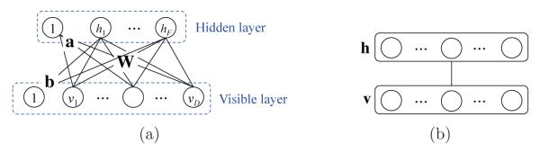
An architecture of a restricted Boltzmann machine (a) and its simplified representation (b).
In RBM, a joint probability of (v, h) is given by:
| (1) |
where Θ = {W = [Wij] ∈ RD×F, a = [ai] ∈ RD, b = [bj] ∈ RF}, E(v, h; Θ) is an energy function, and Z(Θ) is a partition function that can be obtained by summing over all possible pairs of v and h. For the sake of simplicity, by assuming binary visible and hidden units, the energy function E(v, h; Θ) is defined by
| (2) |
The conditional distribution of the hidden variables given the visible variables and also the conditional distribution of the visible variables given the hidden variables are, respectively, computed as follows:
| (3) |
| (4) |
where is a logistic sigmoid function. Due to the unobservable hidden variables, the objective function is defined as the marginal distribution of the visible variables as follows:
| (5) |
In our work, the observed patch values from MRI and PET are real-valued v ∈ RD. For this case, it is common to use a Gaussian RBM (Hinton and Salakhutdinov, 2006), in which the energy function is given by
| (6) |
where σi denotes a standard deviation of the i-th visible variable and Θ = {W, a, b, σ = [σi] ∈ RD}. This variation leads to the following conditional distribution of visible variables given the binary hidden variables
| (7) |
3.2.2. Deep Boltzmann Machine
A DBM is an undirected graphical model, structured by stacking multiple RBMs in a hierarchical manner. That is, a DBM contains a visible layer v and a series of hidden layers h1 ∈ {0, 1}F1, · · · , hi ∈ {0, 1}Fi, · · · , hL ∈ {0, 1}FL, where Fi denotes the number of units in the i-th hidden layer and L is the number of hidden layers. We should note that, hereafter, for simplicity, we omit bias terms and assume that the visible and hidden variables are binary9 or probability, and the following description on DBM is based on Salakhutdinov and Hinton’s work (Salakhutdinov and Hinton, 2012).
Thanks to the hierarchical nature in the deep network, one of the most important characteristics of the DBM is to capture highly non-linear and complicated patterns or statistics such as the relations among input values. Another important feature of the DBM is that the hierarchical latent feature representation can be learned directly from the data without human intervention. In other words, unlike the previous methods that mostly considered hand-crafted/predefined features (Zhang et al., 2011; Fan et al., 2007b; Liu et al., 2013) or outputs from the predefined functions (Dinov et al., 2005; Hackmack et al., 2012), we assign the role of determining feature representations to a DBM and find them autonomously from the training samples. Utilizing its representational and self-taught learning properties, we can find a latent representation of the original GM tissue intensities and/or PET voxel intensities in a patch. When an input patch is presented to a DBM, the different layers of the network represent different levels of information. That is, the lower the layer in the network, the simpler patterns (e.g., linear relations of input variables); the higher the layer, the more complicated or abstract patterns inherent in the input values (e.g., non-linear relations among input variables).
The rationale of using DBM for feature representation is as follows: (1) It can learn internal latent representations that capture non-linear complicated patterns and/or statistical structures in a hierarchical manner (Bengio, 2009; Bengio et al., 2007; Hinton et al., 2006; Mohamed et al., 2012). However, unlike many other deep network models such as deep belief network (Hinton and Salakhutdinov, 2006), and stacked auto-encoder (Shin et al., 2013), the approximate inference procedure after the initial bottom-up pass incorporates top-down feedback, which allows DBM to use higher-level knowledge to resolve uncertainty about intermediate-level features, thus creating better data-dependent representations and statistics for learning (Salakhutdinov and Hinton, 2012). Thanks to this two-way dependencies, i.e., bottom-up and top-down, it was shown that DBMs outperform the other deep learning methods in computer vision (Salakhutdinov and Hinton, 2009; Montavon et al., 2012; Srivastava and Salakhutdinov, 2012). To this end, we use a DBM to discover hierarchical feature representation from neuroimaging, e.g., MRI and PET in our work.
Fig. 3(a) shows an example of the three-layer DBM. The energy of the state (v, h1, h2) in the DBM is given by
| (8) |
where and are, respectively, symmetric connections of (v, h1) and (h1, h2), and Θ = {W1, W2}. Then the probability that the model assigns to a visible vector v is given by:
| (9) |
where Z(Θ) is a normalizing factor. Given the values of the units in the neighboring layer(s), the probability of the binary visible or binary hidden units being set to 1 is computed as follows:
| (10) |
| (11) |
| (12) |
Note that in the computation of the probability of the hidden units h1, we incorporate both the lower visible layer v and the higher hidden layer h2, and this makes DBM differentiated from other deep learning models and also more robust to noisy observations (Salakhutdinov and Hinton, 2009; Srivastava and Salakhutdinov, 2012).
Figure 3.

An architecture of (a) a conventional deep Boltzmann machine and (b) its discriminative version with label information at the top layer.
Unlike the conventional generative DBM, in this work, we consider a discriminative DBM, by injecting a discriminative RBM (Larochelle and Bengio, 2008) at the top hidden layer. That is, the top hidden layer is connected to both the lower hidden layer and the additional label layer (Fig 3(b)), which indicates the label of the input v. In this way, we can train DBM to discover hierarchical and discriminative feature representations by integrating the process of discovering features of inputs with their use in classification (Larochelle and Bengio, 2008). Our model does not require an additional fine-tuning step for classification as done in (Salakhutdinov and Hinton, 2009; Ngiam et al., 2011). With the inclusion of the additional label layer, the energy of the state (v, h1, h2, o) in the modified DBM is given by
| (13) |
where U = [Ulk] ∈ RC×F2 and o = [ol] ∈ {0, 1}C denote, respectively, a connectivity between the top hidden layer and the label layer and a classlabel indicator vector, C is the number of classes, and Θ = {W1, W2, U}. The probability of an observation (v, o) is computed by
| (14) |
The conditional probability of the top hidden units being set to 1 is given by
| (15) |
For the label layer, we use a logistic function
| (16) |
In this way, the hidden units capture class-predictive information about the input vector. Here, we should note that the label layer connected to the top hidden layer is considered during only the training phase of finding the class-discriminative parameters.
From a feature learning perspective, in the low layer of our model, basic image features such as spots and edges are captured from the input data. The learned low-level features are further fed into the high-level of the network, which encodes more abstract and higher level semantic information inherent in the input data. But, here, we should note that the output layer linked to the top hidden layer imposes the learned features to be discriminative between classes.
In order to learn the parameters Θ = {W1, W2, U}, we maximize the log-likelihood of the observed data (v, o). The derivative of the log-likelihood of the observed data with respect to the model parameters takes the simple form of
| (17) |
| (18) |
where < · >data denotes the data-dependent statistics obtained by sampling the model conditioned on the visible units v(≡ h0) and the label units o clamped to the observation and the corresponding label, respectively, and < · >model denotes the data-independent statistics obtained by sampling from the model. When the model approximates the data distribution well, it can be reached for the equilibrium of data-dependent and data-independent statistics. In parameters learning, we use a gradient-based optimization strategy. In Eq. (17) and Eq. (18), we need to compute the data-dependent and the data-independent statistics. First, because of the two-way dependency in DBM, it is not tractable for the data-dependent statistics. Fortunately, variational mean-field approximation works well for estimating the data-dependent statistics. For the details of computing the data-dependent statistics, please refer to Appendix A and (Salakhutdinov and Hinton, 2012).
Here, we should note that due to the large number of parameters involved in the DBM, it generally requires a huge number of training samples for generalization, which is not valid in practice, especially for the neuroimaging studies. However, Hinton et al. recently introduced a greedy layer-wise learning algorithm and successfully applied to learn a deep belief network (Hinton and Salakhutdinov, 2006). Since the pioneering work, many research groups have used this approach to initialize the parameters in deep learning and called it ‘pre-training’ (Hinton et al., 2006; Bengio, 2009). We apply the same procedure to provide a good initial configuration of the parameters, which helps the learning procedure converge much faster than random initialization. The key idea in a greedy layer-wise learning is to train one layer at a time by maximizing the variational lower bound. That is, we first train the 1st hidden layer with the training data as input, and then train the 2nd hidden layer with the outputs from the 1st hidden layer as input, and so on. That is, the representation of the l-th hidden layer is used as input for the (l + 1)-th hidden layer and this pairwise model becomes an RBM. Here, it should be mentioned that, unlike the other deep networks, because the DBM integrates both bottom-up and top-down information, the first and last RBMs in the network need modification by using weights twice as big as in one direction. Since the detailed explanation on this issue is out of domain of our work, please refer to (Salakhutdinov and Hinton, 2012) for details.
In a nutshell, the learning proceeds by two steps: (1) a greedy-layer-wise pre-training for a good initial setup of the modal parameters, and (2) iterative alternation of variational mean-field approximation to estimate the posterior probabilities of hidden units and stochastic approximation to update model parameters (refer to Appendix A). After learning the parameters, we can then obtain a latent feature representation for an input sample, by inferring the probabilities of the hidden units in the trained DBM10.
3.3. Multimodal Deep Feature Fusion
There are increasing evidences that biomarkers from different modalities can provide complementary information in AD/MCI diagnosis (Perrin et al., 2009; Kohannim et al., 2010; Hinrichs et al., 2011; Zhang et al., 2011; Suk and Shen, 2013). Unlike the previous methods that either simply concatenated features from multiple modalities into a long vector (Kohannim et al., 2010) or fused the modality-dependent features in a kernel space (Hinrichs et al., 2011; Zhang et al., 2011; Suk and Shen, 2013), in this work, we propose a systematic method of extracting multimodal feature representations in a probabilistic manner.
Different modalities will have different statistical properties, thus making it difficult to jointly model them using a shallow architecture. Therefore, simple concatenation of the features of multiple modalities can cause strong connections among the variables of individual modality, but few units across modalities (Ngiam et al., 2011). In order to tackle this problem, Srivastava and Salakhutdinov proposed a MultiModal DBM (MM-DBM) to combine images and texts for information retrieval (Srivastava and Salakhutdinov, 2012). Motivated by their work, in this paper, we devise a modified MM-DBM, in which the top hidden layer has multiple entries of the lower hidden layers and the label layer, to extract a shared feature representation by fusing neuroimaging information of MRI and PET. Fig. 4 presents a multimodal deep network in which one path represents the statistical properties of MRI and the other path represents those of PET, and the top shared hidden layer finally discovers the shared properties of the modalities in a supervised manner. We argue that this joint feature representation discriminates our method from the previous multimodal methods (Hinrichs et al., 2011; Zhang et al., 2011; Suk and Shen, 2013), which first extracted features from each modality independently, and then combined them through kernel machines.
Figure 4.

An architecture of a multimodal deep Boltzmann machine for neuroimaging data fusion.
The joint distribution over the multimodal inputs of MRI and PET can be estimated as follows:
| (19) |
where the subscripts M, P, and S denote, respectively, units of the MRI path, the PET path, and the shared hidden layer. Regarding parameters learning for MM-DBM, the same strategy with the unimodal DBM learning can be applied. For details, please refer to Appendix B.
3.4. Image-Level Hierarchical Classifier Learning
In order to combine the distributed patch information over an image and build an image-level classifier, we use a hierarchical classifier learning scheme, proposed by Liu et al. (Liu et al., 2013). That is, we first build a classifier for each patch, independently, and then combine them in a hierarchical manner by feeding the outputs from the lower-level classifiers to the upper-level classifier. Specifically, we build a three-level classifier for decision: patch-level, mega-patch-level, and image-level. For the patch-level classification, a linear Support Vector Machine (SVM) is trained for each patch location independently with the (MM-)DBM-learned feature representations as input. The output from a patch-level SVM, measured by the relative distance from the decision hyperplane, is then converted to a probability via a soft-max function. Here, we should note that in patch-level classifier learning, we randomly partition the training data into a training set and a validation set1. The patch-level classifier is trained on the training set, and then the classification accuracy is obtained with the validation set.
In the following hierarchy, instead of considering all patch-level classifiers’ output simultaneously, we agglomerate the information of the locally distributed patches by constructing spatially distributed ‘mega-patches’ under the consideration that the disease-related brain areas are distributed over some distant brain regions with arbitrary shape and size (Liu et al., 2013). Similar to the patch extraction described in Section 3.1, we construct mega-patches and the respective classifiers in a greedy manner. Concretely, we first sort the patches in a descending order based on the classification accuracy obtained with the validation set in patch-level classifier learning. Starting with the patch with the highest classification accuracy as a new mega-patch, we greedily merge the neighboring patches into the mega-patch. The merging condition is that, if and only if, a mega-patch classifier, which is trained with the patches already included in the current mega-patch and also the candidate patch under consideration, produces a better classification accuracy. The process is repeated until all the patches are visited. The size of the constructed mega-patches and their component-patches are determined by a cross-validation. We also constrain that none of the final mega-patches overlap each other larger than the half of the respective mega-patches’ size. Note that, in the step of the mega-patch classifier learning, some patches that are not informative in classification are discarded, and each mega-patch classifier covers different regions of the brain with a different size.
Finally, we build an image-level classifier by fusing the mega-patch classifiers. We select an optimal subset of mega-patches in a forward greedy search strategy for a final fusion. However, since the mega-patch selection is performed on the training data, the resulting image-level classifier may not be optimal for the testing data. To this end, we divide the training data into multiple subsets, and train an image-level classifier in each subset individually12. In this way, we can build multiple image-level classifiers, each of which selects possibly a different subset of mega-patches. By counting the selected frequency of mega-patches in each image-level classifier, we can finally compute the relative importance of the mega-patches. After normalizing the frequencies, we use them as weights of the respective mega-patches. The final decision in image-level classifiers is made by a weighted combination of the mega-patch classifiers’ outputs.
4. Experimental Results and Discussions
In this section, we evaluate the effectiveness of the proposed method for (1) a latent feature representation with DBM and (2) a shared feature representation between MRI and PET with an MM-DBM, by considering three binary classification problems: AD vs. NC, MCI vs. NC, MCI converter (MCI-C) vs. MCI non-converter (MCI-NC). Due to the limited number of data, we applied a 10-fold cross validation technique. Specifically, we randomly partitioned the dataset into 10 subsets, each of which included 10% of the total data. We repeated experiments for each classification problem 10 times, by using 9 out of 10 subsets for training and the remaining one for testing at each time. It is worth noting that, for each classification problem, during a training phase, we performed patch selection, (MM-)DBM and SVM model learning only using the 9 training subsets. Based on the selected patches and also the trained (MM-)DBM and SVM models, we finally evaluated the performance on the left-out testing subset. We compare the proposed method with Liu et al.’s method (Liu et al., 2013), using the same training and testing set in each experiment for a fair comparison.
4.1. Experimental Setup
As for the patch size w, we set it to 11 by following Liu et al.’s work (Liu et al., 2013). During mega-patch construction, the size of a mega-patch was allowed in the range of w × [1.2, 1.4, 1.6, 1.8, 2] and the optimal size for each mega-patch was determined by cross-validation as explained in Section 3.4.
In building (MM)-DBM of GM patches and/or PET patches, we can use Gaussian visible units for the input patches by considering the voxels as continuous variables. However, learning (MM-)DBMs with Gaussian visible units is very slow and requires a huge number of parameter updates, compared with the binary visible units. To this end, we first trained RBM with 1, 331(= 113) Gaussian visible units and also 500 binary hidden units by using contrastive divergence learning (Hinton et al., 2006) for 1000 epochs13. After training a Gaussian RBM for each modality, we used it as a preprocessor, following Nair and Hinton’s work (Nair and Hinton, 2008), that effectively converts GM tissue densities or PET voxel intensities into 500-dimensional binary vectors. We then used the binary vectors as ‘preprocessed data’ to train our (MM-)DBMs. We should note that the Gaussian RBMs were not updated during (MM-)DBMs learning.
We structured a three-layer DBM for MRI (MRI-DBM) and PET (PET-DBM), respectively, and a four-layer DBM for MRI+PET (MM-DBM). For all these models, we used binary visible and binary hidden units. Both the MRI-DBM and the PET-DBM were structured with 500(visible)-500(hidden)-500(hidden), and the MM-DBM was structured with 500(visible)-500(hidden)-500(hidden) for a MRI pathway, 500(visible)-500(hidden)-500(hidden) for a PET pathway, and finally 1,000 hidden units for the shared hidden layer. In (MM-)DBM learning, we updated the parameters, i.e., weights and biases, with a learning rate of 10−3 and a momentum of 0.5 with an increment gradually up to 0.9 for 500 epochs. We used the trained parameters of MRI-DBM and PET-DBM as the initial setup of the MRI and PET pathways in MM-DBM learning. We implemented the DBM method based on Salakhutdinov’s codes14.
We used a linear SVM for the hierarchical classifiers, i.e., patch-level classifier, mega-patch-level classifier, and image-level classifier. An LIBSVM toolbox15 was used for SVM learning and classification. The free parameter that controls the soft margin was determined by a nested cross-validation.
4.2. Extracted Patches and Trained DBMs
In Fig. 5, we presented the example images overlaid with p-values of the voxels, obtained from AD and NC groups, based on which we selected patch locations for AD and NC classification. It is worth noting that, for both modalities, the voxels in the subcortical and medial temporal areas showed low p-values, i.e., statistically different between classes, while for other areas, each modality presents slightly different p-value distributions, from which we could possibly obtain complementary information for classification. Samples of the selected 3D patches are also presented in Fig. 6, in which one 3D volume is displayed in each row, for each modality. Taking these patches as input data to a Gaussian RBM and then transforming to binary vectors, we trained our feature representation models, i.e., MRI-DBM, PET-DBM, and MM-DBM. Regarding the trained MM-DBM, we visualized the trained weights in Fig. 7 by linearly projecting them to the input space for intuitive interpretation of the feature representations16. In the figure, the left images represent the trained weights of our Gaussian RBMs that were used to convert the real-valued patches into binary vectors as a preprocessor, and the right images represent the trained weights of the first-layer hidden units of the respective modality’s pathway in our MM-DBM. From the figure, we can regard the hidden units in the Gaussian RBM as simple cells of a human visual cortex that maximally responds to specific spot- or edge-like stimulus patterns within the receptive field, i.e., a patch in our case. In particular, each hidden unit in a Gaussian RBM finds simple volumetric or functional patterns in the input 3D patch by assigning different weights to the corresponding voxels. For example, hidden units of the Gaussian RBM for MRI (left in Fig. 7(a)) focus on different parts of a patch to detect a simple spot- or edge-like pattern in the input 3D GM patch. The hidden units in a Gaussian RBM for PET (left in Fig. 7(b)) can be understood as descriptors that discover local functional relations among voxels within a patch.
Figure 5.

Visualization of the p-value distributions used to select the patch locations of MRI and PET in AD and NC classification.
Figure 6.

Samples of the selected patches, whose voxel values are the input to the (MM-)DBM.
Figure 7.

Visualization of the trained weights of our modality-specific Gaussian RBMs (left) used for data conversion from a real-valued vector to a binary vector, and those of our MM-DBM (right) used for latent feature representations. For the weights of our MM-DBM, they correspond to the first hidden layer in the respective modality’s pathway in the model. In each subfigure, one row corresponds to one hidden unit in the respective Gaussian RBM or MM-DBM.
Note that the hidden units of a Gaussian RBM for either MRI or PET find, respectively, the structural or functional relations among voxels in a localized way. Meanwhile, the hidden units in our (MM-)DBM served as complex filters of a human visual cortex that combine the outputs from the simple cells and maximally responds to more complex patterns within the receptive field. For example, the weights of hidden units in the hidden layer of the MRI pathway in an MM-DBM (right in Fig. 7(a)) discover more complicated structural patterns in the input 3D GM patch, such as combination of edges orienting in different directions. With respect to the PET, the weights of hidden units in the hidden layer of the PET pathway in an MM-DBM (right in Fig. 7(b)) discover non-linear functional relations among voxels within a 3D patch. In this way, as it forwards to the higher layer, the (MM-)DBM finds complex latent features in the input patch, and ultimately in the top hidden layer, the hidden units discover the inter-modality relations in between the pair of MRI and PET patches, each of which comes from the same location in a brain.
4.3. Performance Evaluation
Let TP, TN, FP, and FN denote, respectively, True Positive, True Negative, False Positive, and False Negative. In this work, we consider the following quantitative measurements and presented the performances of the competing methods in Table 2.
Table 2.
A summary of the performances of two methods.
| Method | Modality | ACC (%) |
SEN (%) |
SPEC (%) |
BAC (%) |
PPV (%) |
NPV (%) |
AUC | |
|---|---|---|---|---|---|---|---|---|---|
| AD/NC | Liu et al. | MRI | 90.18±5.25 | 91.54 | 90.61 | 91.08 | 88.94 | 90.67 | 0.9620 |
| PET | 89.13±6.81 | 90.06 | 89.36 | 89.71 | 88.49 | 89.26 | 0.9594 | ||
| MRI+PET | 90.27±7.02 | 89.48 | 92.44 | 90.96 | 90.56 | 88.70 | 0.9655 | ||
| Proposed | MRI | 92.38±5.32 | 91.54 | 94.56 | 93.05 | 92.65 | 90.84 | 0.9697 | |
| PET | 92.20±6.70 | 88.04 | 96.33 | 92.19 | 95.03 | 89.66 | 0.9798 | ||
| MRI+PET | 95.35±5.23 | 94.65 | 95.22 | 94.93 | 96.80 | 95.67 | 0.9877 | ||
| MCI/NC | Liu et al. | MRI | 81.00±4.98 | 97.08 | 48.18 | 72.63 | 79.14 | 88.99 | 0.8352 |
| PET | 81.14±10.22 | 96.03 | 52.59 | 74.31 | 80.26 | 84.16 | 0.8231 | ||
| MRI+PET | 83.90±5.80 | 98.97 | 52.59 | 75.78 | 81.18 | 97.22 | 0.8301 | ||
| Proposed | MRI | 84.24±6.26 | 99.58 | 53.79 | 76.69 | 81.23 | 98.75 | 0.8478 | |
| PET | 84.29±7.22 | 98.69 | 56.87 | 77.78 | 81.99 | 94.57 | 0.8297 | ||
| MRI+PET | 85.67±5.22 | 95.37 | 65.87 | 80.62 | 85.02 | 89.00 | 0.8808 | ||
| MCI-C/MCI-NC | Liu et al. | MRI | 64.75± 14.83 | 22.22 | 89.57 | 55.90 | 46.29 | 77.39 | 0.6355 |
| PET | 67.17±13.43 | 40.02 | 82.61 | 61.32 | 64.13 | 70.31 | 0.6911 | ||
| MRI+PET | 73.33±12.47 | 33.25 | 97.52 | 65.38 | 80.00 | 73.18 | 0.7159 | ||
| Proposed | MRI | 72.42±13.09 | 36.70 | 90.98 | 63.84 | 65.49 | 77.84 | 0.7342 | |
| PET | 70.75±13.23 | 25.45 | 96.55 | 61.00 | 75.00 | 70.69 | 0.7215 | ||
| MRI+PET | 75.92±15.37 | 48.04 | 95.23 | 71.63 | 83.50 | 74.33 | 0.7466 |
ACCuracy (ACC) = (TP+TN) / (TP+TN+FP+FN)
SENsitivity (SEN) = TP / (TP+FN)
SPECificity (SPEC) = TN / (TN+FP)
Balanced ACcuracy (BAC) = (SEN+SPEC) / 2
Positive Predictive Value (PPV) = TP / (TP+FP)
Negative Predictive Value (NPV) = TN / (TN+FN)
Area Under the receiver operating characteristic Curve (AUC)
In the classification of AD and NC, the proposed method showed the mean accuracies of 92.38% (MRI), 92.20% (PET), and 95.35% (MRI+PET). Compared to Liu et al.’s method that showed the accuracies of 90.18% (MRI), 89.13% (PET), and 90.27% (MRI+PET)17, the proposed method improved by 2.2% (MRI), 3.07% (PET), and 5.08% (MRI+PET). That is, the proposed method outperformed Liu et al.’s method in all the cases of MRI, PET, and MRI+PET. In the discrimination of MCI from NC, the proposed method showed the accuracies of 84.24% (MRI), 84.29% (PET), and 85.67% (MRI+PET). Meanwhile, Liu et al.’s method showed the accuracies of 81% (MRI), 81.14% (PET), and 83.90% (MRI+PET). Again, the proposed method outperformed Liu et al.’s method by making performance improvements of 3.24% (MRI), 3.15% (PET), and 1.77% (MRI+PET). In the classification between MCI-C and MCI-NC, which is the most important for early diagnosis and treatment, Liu et al.’s method achieved the accuracies of 64.75% (MRI), 67.17% (PET), and 73.33% (MRI+PET). Compared to these results, the proposed method improved the accuracies by 7.67% (MRI), 3.58% (PET), and 2.59% (MRI+PET), respectively. Concisely, in our three binary classifications, based on the classification accuracy, the proposed method clearly outperformed Liu et al.’s method by achieving the maximal accuracies of 95.35% (AD vs. NC), 85.67% (MCI vs. NC), and 75.92% (MCI-C vs. MCI-NC), respectively.
Regarding sensitivity and specificity, the higher the sensitivity, the lower the chance of mis-diagnosing AD/MCI patients; also the higher the specificity, the lower the chance of mis-diagnosing NC to AD/MCI. Although the proposed method had a lower sensitivity than that of Liu et al.’s method for a couple of cases, e.g., 90.06% (Liu et al.’s method) vs. 88.04% (proposed) with PET in the AD diagnosis, 98.97% (Liu et al.’s method) vs. 95.37% (proposed) with MRI+PET in the MCI diagnosis, and 40.02% (Liu et al.’s method) vs. 25.45% (proposed) with PET in the MCI-C diagnosis, in general, the proposed method showed higher sensitivity and specificity in all three classification problems. Hence, from a clinical point of view, the proposed method is less likely to mis-diagnose subjects with AD/MCI and vice versa, compared to Liu et al.’s method.
Meanwhile, because of the data imbalance between classes, i.e., AD (93 subjects), MCI (204 subjects; 76 MCI-C and 128 MCI-NC subjects), and NC (101 subjects), we obtained low sensitivity (MCI vs. NC) or specificity (MCIC vs. MCI-NC). The balanced accuracy, which is calculated by taking the average of sensitivity and specificity, avoids inflated performance estimates on imbalanced datasets. Based on this metric, we clearly see that the proposed method is superior to the competing method. Note that in discrimination between MCI and NC, while the accuracy improvement by the proposed method with MRI+PET was 1.43% and 1.38% compared to the same method with MRI and PET, respectively, in terms of the balanced accuracy, the improvements went up to 3.93% (vs. MRI) and 2.95% (vs. PET).
With a further concern on low sensitivity and specificity, especially in classifications of MCI vs. NC and MCI-C vs. MCI-NC, we also computed a Positive Predictive Value (PPV) and a Negative Predictive Value (NPV). Statistically, PPV and NPV measure, respectively, the proportion of subjects with AD, MCI, or MCI-C who are correctly diagnosed as patients, and the proportion of subjects without AD, MCI, or MCI-C who are correctly diagnosed as cognitive normal. Based on a recent report by Alzheimer’s Association (Alzheimer’s Association, 2012), the AD prevalence is projected to be 11 millions to 16 millions by 2050. For MCI and MCI-C, although there is high variation among reports depending on definitions, the median of the prevalence estimates of MCI or MCI-C in the literature is 26.4% (MCI) and 4.9% (amnestic MCI) (Ward et al., 2012). Regarding the AD prevalence by 2050, the proposed method, which achieved 96.80% of the PPV in the classification of AD and NC, can correctly identify 10.648 millions to 15.488 millions of subjects with AD while Liu et al.’s method, whose respective PPV was 90.56%, can identify 9.9616 millions to 14.4896 millions of subjects with AD. Accordingly, our method can correctly identify as many as 0.6864 millions to 0.9984 millions of subjects more.
The Receiver Operating Characteristic (ROC) curve18 and the Area Under the ROC Curve (AUC) are also widely used metrics to evaluate the performance of diagnostic tests in brain disease as well as other medical areas. In particular, the AUC can be thought as a measure of the overall performance of a diagnostic test. The proposed method with MRI+PET showed the best AUCs of 0.9877 in AD vs. NC, 0.8808 in MCI vs. NC, and 0.7466 in MCI-C vs. MCI-NC. Compared to Liu et al.’s method with MRI+PET, the proposed multimodal method increased the AUCs by 0.0222 (AD vs. NC), 0.0507 (MCI vs. NC), and 0.0307 (MCI-C vs. MCI-NC). Noticeably, the proposed method with MRI enhanced the AUC as much as 0.0987 than the corresponding AUC of Liu et al.’s method. It is also noteworthy that in the classification of MCI and NC, the proposed method with MRI+PET improved the AUC by 0.0330 (vs. MRI) and 0.0389 (vs. PET), while the improvements in the classifications of AD vs. NC and MCI-C vs. MCI-NC were, respectively, 0.0180/0.0079 (vs. MRI/PET) and 0.0124/0.0251 (vs. MRI/PET).
Based on the quantitative measurements depicted above, the proposed method clearly outperforms Liu et al.’s method. In terms of modalities used for classification, similar to the previous work (Hinrichs et al., 2011; Zhang et al., 2011; Suk and Shen, 2013), we also obtained the best performances with the complementary information from multiple modalities, i.e., MRI+PET.
4.4. Comparison with State-of-the-Art Methods
In Table 3, we also compared the classification accuracies of the proposed method with those of the state-of-the-art methods that considered multi-modality in classifications of AD vs. NC, MCI vs. NC, and MCI-C vs. MCI-NC. Note that, due to different datasets and different approaches of extracting features and building classifiers, it is not fair to directly compare the performances among methods. Nonetheless, it is remarkable that the proposed method showed the highest accuracies among the methods in all the binary classification problems. It is also worth noting that our method is the only one that considered the patch-based approach for feature extraction, while the other methods used an ROI-based approach.
Table 3.
Comparison of classification accuracy with state-of-the-art methods. The numbers in the parentheses denote the number of AD/MCI(MCI-C,MCI-NC)/NC subjects in the dataset used.
| Methods | Dataset | Features | AD vs. NC (%) |
MCI vs. NC (%) |
MCI-C vs. MCI-NC (%) |
|---|---|---|---|---|---|
| (Kohannim et al., 2010) | MRI+PET+CSF (40/83(43,40)/43) |
ROI | 90.7 | 75.8 | n/a |
| (Walhovd et al., 2010) | MRI+CSF (38/73/42) |
ROI | 88.8 | 79.1 | n/a |
| (Hinrichs et al., 2011) | MRI+PET | ROI (48/119(38,81)/66) |
92.4 | n/a | 72.3 |
| (Westman et al., 2012) | MRI+CSF | ROI (96/162(81,81)/111) |
91.8 | 77.6 | 66.4 |
| (Zhang and Shen, 2012) | MRI+PET+CSF (45/91(43,48)/50) |
ROI | 93.3 | 83.2 | 73.9 |
| Proposed method | MRI+PET (93/204(76,128)/101) |
Patch | 95.35 | 85.67 | 75.92 |
4.5. Importance of Brain Areas in Classification
For the investigation of the relative importance of different brain areas determined by the proposed method for AD/MCI diagnosis, we visualized the weights of the selected patches in Fig. 8. Specifically, the weight of each patch was calculated by accumulating the selected frequency of mega-patches in final ensemble classifiers over cross-validations. That is, the weight of a patch was determined with the sum of the weights of the mega-patches that included the patch and was used in the final decision. The high weighted patches were in accordance with the previous reports on AD/MCI studies. Those were distributed around a medial temporal lobe (that includes amygdala, hippocampal formation, entorhinal cortex) (Braak and Braak, 1991; Visser et al., 2002; Mosconi, 2005; Lee et al., 2006; Devanand et al., 2007; Burton et al., 2009; Desikan et al., 2009; Ewers et al., 2012; Walhovd et al., 2010), superior/medial frontal gyrus (Johnson et al., 2005), precentral/postcentral gyrus (Belleville et al., 2011), precuneus (Bokde et al., 2006; Singh et al., 2006; Davatzikos et al., 2011), thalamus, putamen (de Jong et al., 2008), caudate nucleus (Dai et al., 2009), etc.
Figure 8.

Patch weight distributions in classification of AD vs. NC and MCI vs. NC.
4.6. Limitations
In our experiments, we validated the efficacy of the proposed method in three classification problems by achieving the best performances. However, there still exist some limitations of the proposed method.
First, even though we could visualize the trained weights in our (MM-)DBMs in Fig. 7, from a clinical perspective, it is difficult to understand or interpret the resulting feature representations. Particularly, with respect to the investigation of brain abnormalities affected by neurodegenerative disease, i.e., AD or MCI, our method cannot provide useful clinical information. In this regard, it could be a good research direction in which we further extend the proposed method to find or detect brain abnormalities in terms of brain regions or areas for easy understanding to clinicians.
Second, in our experiments, we manually determined the number of hidden units in each layer. Furthermore, we used a relatively small data samples (93 AD, 76 MCI-C, 128 MCI-NC, and 101 NC). Therefore, the network structures used to discover high-level feature representations in our experiments were not necessarily optimal. We believe that it needs more intensive studies such as learning the optimal network structure from big data for practical use of deep learning in clinical settings.
Third, as the graphical model illustrated in Fig. 4, the current method only considers bi-modalities of MRI and PET. However, it is generally beneficiary to combine as many modalities as possible to use their richer information. Therefore, it is necessary to build a more systematic model that can efficiently find and use complementary information from genetics, proteomics, imaging, cognition, disease status, and other phenotypic modalities.
Lastly, according to a recent broad spectrum of studies, there are increasing evidences that subjective cognitive complaint is one of the important genetic risk factors, which increases the risk of progression to MCI or AD (Loewenstein et al., 2012; Mark and Sitskoorn, 2013). That is, among the cognitively normal elderly individuals who have subjective cognitive impairments, there exists a high possibility for some of them to be in the stage of ‘pre-MCI’. However, in the ADNI dataset, there is no related information. Thus, in our experiments, the NC group could include both genuine controls and those with subjective cognitive complaints.
5. Conclusions
In this paper, we proposed a method for a shared latent feature representation from MRI and PET in deep learning. Specifically, we used DBM to find a latent feature representation from a volumetric patch and further devised method to systemically discover a joint feature representation from multi-modality. Unlike the previous methods that mostly considered the direct use of the GM tissue densities from MRI and/or voxel intensities from PET and then fused the complementary information in a kernel technique, the proposed method learned high-level features in a self-taught manner via deep learning, and thus could efficiently combine the complimentary information from MRI and PET during feature representation procedure. Experimental results on ADNI dataset showed that the proposed method is superior to the previous methods in terms of various quantitative metrics.
Highlights.
A novel method for a high-level latent feature representation from neuroimaging data
A systematic method for joint feature representation of multimodal neuroimaging data
Hierarchical patch-level information fusion via an ensemble classifier
Maximal diagnostic accuracies of 93.52% (AD vs. NC), 85.19% (MCI vs. NC), and 74.58% (MCI converter vs. MCI non-converter)
Acknowledgement
This work was supported in part by NIH grants EB006733, EB008374, EB009634, AG041721, MH100217, and AG042599, and also by the National Research Foundation grant (No. 2012-005741) funded by the Korean government.
Appendix A. Variational Approximation for DBM Learning
The main idea of applying variational approximation is to assume that the true posterior distribution over latent variables P(h1, h2∣v; Θ) for each training vector v is unimodal and can be replaced by an approximate posterior Q(h1, h2∣v; Ω), which can be computed efficiently, and the parameters are updated to maximize the variational lower bound on the log-likelihood
| (A.1) |
| (A.2) |
where H(·) is the entropy functional, KL[·∥·] denotes Kullback-Leibler divergence, and ω is a variational parameter set. For computational simplicity and learning speed, the naïve mean-field approximation, which uses a fully factorized distribution, is generally used in the literature (Tanaka, 1998). That is, where
| (A.3) |
where , , , , and . It alternatively estimates the state of the hidden units, μ1 and μ2, for fixed Θ until convergence:
| (A.4) |
| (A.5) |
Regarding the data-independent statistics, we apply a stochastic approximation procedure to obtain samples, also called particles, of , , and by running repeatedly the alternate Gibbs sampler on a set of particles. Once both the data-dependent and data-independent statistics are computed, we then update parameters as follows:
| (A.6) |
| (A.7) |
| (A.8) |
where αt is a learning rate, and N and M denote, respectively, the numbers of training data and particles, and superscripts n and m denote, respectively, indices of an observation and a particle.
Appendix B. Learning Multimodal DBM Parameters
The same approach to the unimodal DBM described in Section 3.2.2 can be applied, i.e., iterative alternation of the variational mean-field approximation for data-dependent statistics and the stochastic approximation procedure for data-independent statistics, and parameters update. Let and V = {vM, vP}. In variational learning of our MM-DBM, a fully factorized mean-field variational function for approximation of the true posterior distribution is defined as follows:
| (B.1) |
where is a mean-field parameter set with , , , , and . Referring Eq. (A.4) and Eq. (A.5), given a fixed model parameter Θ, it is straightforward to estimate the mean-field parameters Ω.
The learning proceeds by iteratively alternating the variational mean-field inference to find the values of Ω for the fixed current model parameters Θ and the stochastic approximation procedure to update model parameters Θ given the variational parameters Ω. Finally, the shared feature representations can be obtained by inferring the values of the hidden units in the top hidden layer from the trained MM-DBM.
Footnotes
Publisher's Disclaimer: This is a PDF file of an unedited manuscript that has been accepted for publication. As a service to our customers we are providing this early version of the manuscript. The manuscript will undergo copyediting, typesetting, and review of the resulting proof before it is published in its final citable form. Please note that during the production process errors may be discovered which could affect the content, and all legal disclaimers that apply to the journal pertain.
Although it is clear from the context that the acronym DBM denotes “Deep Boltzmann Machine” in this paper, we would clearly indicate that DBM here is not related to “Deformation Based Morphometry”.
Available at ‘http://www.loni.ucla.edu/ADNI’.
Although there exist in total more than 800 subjects in ADNI database, only 398 subjects have the baseline data including the modalities of both MRI and FDG-PET.
Refer to ‘http://www.adniinfo.org’ for the details.
Available at ‘http://mipav.cit.nih.gov/clickwrap.php’.
Available at ‘http://fsl.fmrib.ox.ac.uk/fsl/fslwiki/’.
The final voxel size is 4×4×4 mm3.
In this work, we set the threshold to 0.05.
In our experiments, we trained a Gaussian RBM by fixing the standard deviations to 1 and transformed the observed real-values from MRI and PET to binary vectors using it as a preprocessor, following Nair and Hinton’s work (Nair and Hinton, 2008).
Instead of the standard mean-field approximation, inspired by Montavon et al.’s work (Montavon et al., 2012), in this work, we traverse the trained DBM in a feed-forward manner, i.e., f = sigm(W2 · sigm(W1v)), for feature representations. The same strategy is applied for the multimodal DBM described in Section 3.3.
In our work, we set 80% of the entire training data as a training set and the rest for a validation set.
In this work, we set the number of subsets to 10.
The input data were first normalized and whitened by zero component analysis, and the standard deviation was fixed to 1 during the parameter updates.
Available at ‘http://www.cs.toronto.edu/~rsalakhu/DBM.html’.
Available at ‘http://www.csie.ntu.edu.tw/~cjlin/libsvm/’.
For the hidden units of the MRI pathway and the PET pathway, their weights were visualized as a weighted linear combination of the weights of the Gaussian RBM, similar to Lee et al.’s work (Lee et al., 2009).
For the multimodal case, we concatenated the patches of modalities into a single vector for Liu et al.’s method.
A plot of test true positive rate versus its false positive rate.
References
- Alzheimer’s Association 2012 Alzheimer’s disease facts and figures. Alzheimer’s & Dementia. 2012;8(2):131–168. doi: 10.1016/j.jalz.2012.02.001. [DOI] [PubMed] [Google Scholar]
- Baron J, Chtelat G, Desgranges B, Perchey G, Landeau B, de la Sayette V, Eustache F. In vivo mapping of gray matter loss with voxel-based morphometry in mild Alzheimer’s disease. NeuroImage. 2001;14(2):298–309. doi: 10.1006/nimg.2001.0848. [DOI] [PubMed] [Google Scholar]
- Belleville S, Clment F, Mellah S, Gilbert B, Fontaine F, Gauthier S. Training-related brain plasticity in subjects at risk of developing Alzheimers disease. Brain. 2011;134(6):1623–1634. doi: 10.1093/brain/awr037. [DOI] [PubMed] [Google Scholar]
- Bengio Y. Learning deep architectures for AI. Foundations and Trends in Machine Learning. 2009;2(1):1–127. [Google Scholar]
- Bengio Y, Lamblin P, Popovici D, Larochelle H. Greedy layer-wise training of deep networks. In: Schölkopf B, Platt J, Ho man T, editors. Advances in Neural Information Processing Systems 19. MIT Press; Cambridge, MA: 2007. pp. 153–160. [Google Scholar]
- Bokde ALW, Lopez-Bayo P, Meindl T, Pechler S, Born C, Faltraco F, Teipel SJ, Möller H-J, Hampel H. Functional connectivity of the fusiform gyrus during a face-matching task in subjects with mild cognitive impairment. Brain. 2006;129(5):1113–1124. doi: 10.1093/brain/awl051. [DOI] [PubMed] [Google Scholar]
- Braak H, Braak E. Neuropathological stageing of Alzheimer-related changes. Acta Neuropathologica. 1991;82(4):239–259. doi: 10.1007/BF00308809. [DOI] [PubMed] [Google Scholar]
- Burton EJ, Barber R, Mukaetova-Ladinska EB, Robson J, Perry RH, Jaros E, Kalaria RN, OBrien JT. Medial temporal lobe atrophy on MRI differentiates Alzheimer’s disease from dementia with lewy bodies and vascular cognitive impairment: a prospective study with pathological verification of diagnosis. Brain. 2009;132(1):195–203. doi: 10.1093/brain/awn298. [DOI] [PubMed] [Google Scholar]
- Catana C, Drzezga A, Heiss W-D, Rosen BR. PET/MRI for neurologic applications. The Journal of Nuclear Medicine. 2012;53:1916–1925. doi: 10.2967/jnumed.112.105346. [DOI] [PMC free article] [PubMed] [Google Scholar]
- Ciresan DC, Giusti A, Gambardella LM, Schmidhuber J. Mitosis detection in breast cancer histology images with deep neural networks. Medical Image Computing and Computer-Assisted Intervention MICCAI 2013. 2013;Vol. 8150 of Lecture Notes in Computer Science:411–418. doi: 10.1007/978-3-642-40763-5_51. [DOI] [PubMed] [Google Scholar]
- Cui Y, Liu B, Luo S, Zhen X, Fan M, Liu T, Zhu W, Park M, Jiang T, Jin JS, the Alzheimer’s Disease Neuroimaging Initiative Identification of conversion from mild cognitive impairment to Alzheimer’s disease using multivariate predictors. PLoS One. 2011;6(7):e21896. doi: 10.1371/journal.pone.0021896. [DOI] [PMC free article] [PubMed] [Google Scholar]
- Cuingnet R, Gerardin E, Tessieras J, Auzias G, Lehéricy S, Habert M-O, Chupin M, Benali H, Colliot O, The Alzheimer’s Disease Neuroimaging Initiative Automatic classification of patients with Alzheimer’s disease from structural MRI: A comparison of ten methods using ADNI database. NeuroImage. 2011;56(2):766–781. doi: 10.1016/j.neuroimage.2010.06.013. [DOI] [PubMed] [Google Scholar]
- Dai W, Lopez O, Carmichael O, Becker J, Kuller L, Gach H. Mild cognitive impairment and Alzheimer disease: patterns of altered cerebral blood flow at MR imaging. Radiology. 2009;250(3):856–866. doi: 10.1148/radiol.2503080751. [DOI] [PMC free article] [PubMed] [Google Scholar]
- Davatzikos C, Bhatt P, Shaw LM, Batmanghelich KN, Trojanowski JQ. Prediction of MCI to AD conversion, via MRI, CSF biomarkers, and pattern classification. Neurobiology of Aging. 2011;32(12):2322.e19–2322.e27. doi: 10.1016/j.neurobiolaging.2010.05.023. [DOI] [PMC free article] [PubMed] [Google Scholar]
- Davatzikos C, Genc A, Xu D, Resnick SM. Voxel-based morphometry using the RAVENS maps: Methods and validation using simulated longitudinal atrophy. NeuroImage. 2001;14(6):1361–1369. doi: 10.1006/nimg.2001.0937. [DOI] [PubMed] [Google Scholar]
- de Jong LW, van der Hiele K, Veer IM, Houwing JJ, Westendorp RGJ, Bollen ELEM, de Bruin PW, Middelkoop HAM, van Buchem MA, van der Grond J. Strongly reduced volumes of putamen and thalamus in Alzheimer’s disease: an MRI study. Brain. 2008;131(12):3277–3285. doi: 10.1093/brain/awn278. [DOI] [PMC free article] [PubMed] [Google Scholar]
- Desikan R, Cabral H, Hess C, Dillon W, Salat D, Buckner R, Fischl B, Initiative ADN. Automated MRI measures identify individuals with mild cognitive impairment and Alzheimer’s disease. Brain. 2009;132:2048–2057. doi: 10.1093/brain/awp123. [DOI] [PMC free article] [PubMed] [Google Scholar]
- Devanand DP, Pradhaban G, Liu X, Khandji A, De Santi S, Segal S, Rusinek H, Pelton GH, Hoing LS, Mayeux R, Stern Y, Tabert MH, de Leon JJ. Hippocampal and entorhinal atrophy in mild cognitive impairment. Neurology. 2007;68:828–836. doi: 10.1212/01.wnl.0000256697.20968.d7. [DOI] [PubMed] [Google Scholar]
- Dinov I, Boscardin J, Mega M, Sowell E, Toga A. A wavelet-based statistical analysis of fMRI data. Neuroinformatics. 2005;3(4):319–342. doi: 10.1385/NI:3:4:319. [DOI] [PubMed] [Google Scholar]
- Ewers M, Walsh C, Trojanowski JQ, Shaw LM, Petersen RC, Jr., C. RJ, Feldman HH, Bokde AL, Alexander GE, Scheltens P, Vellas B, Dubois B, Weiner M, Hampel H. Prediction of conversion from mild cognitive impairment to Alzheimer’s disease dementia based upon biomarkers and neuropsychological test performance. Neurobiology of Aging. 2012;33(7):1203–1214.e2. doi: 10.1016/j.neurobiolaging.2010.10.019. [DOI] [PMC free article] [PubMed] [Google Scholar]
- Fan Y, Rao H, Hurt H, Giannetta J, Korczykowski M, Shera D, Avants BB, Gee JC, Wang J, Shen D. Multivariate examination of brain abnormality using both structural and functional MRI. NeuroImage. 2007a;36(4):1189–1199. doi: 10.1016/j.neuroimage.2007.04.009. [DOI] [PubMed] [Google Scholar]
- Fan Y, Shen D, Gur R, Gur R, Davatzikos C. COMPARE: Classification of morphological patterns using adaptive regional elements. IEEE Transactions on Medical Imaging. 2007b;26(1):93–105. doi: 10.1109/TMI.2006.886812. [DOI] [PubMed] [Google Scholar]
- Friston KJ. Functional and effective connectivity in neuroimaging: A synthesis. Human Brain Mapping. 1995;2:56–78. [Google Scholar]
- Greicius MD, Srivastava G, Reiss AL, Menon V. Default-mode network activity distinguishes Alzheimer’s disease from healthy aging: Evidence from functional MRI. Proceedings of the National Academy of Sciences of the United States of America. 2004;101(13):4637–4642. doi: 10.1073/pnas.0308627101. [DOI] [PMC free article] [PubMed] [Google Scholar]
- Hackmack K, Paul F, Weygandt M, Allefeld C, Haynes J-D. Multi-scale classification of disease using structural MRI and wavelet transform. NeuroImage. 2012;62(1):48–58. doi: 10.1016/j.neuroimage.2012.05.022. [DOI] [PubMed] [Google Scholar]
- Hinrichs C, Singh V, Xu G, Johnson SC. Predictive markers for AD in a multi-modality framework: An analysis of MCI progression in the ADNI population. NeuroImage. 2011;55(2):574–589. doi: 10.1016/j.neuroimage.2010.10.081. [DOI] [PMC free article] [PubMed] [Google Scholar]
- Hinton GE, Osindero S, Teh Y-W. A fast learning algorithm for deep belief nets. Neural Computation. 2006;18(7):1527–1554. doi: 10.1162/neco.2006.18.7.1527. [DOI] [PubMed] [Google Scholar]
- Hinton GE, Salakhutdinov RR. Reducing the dimensionality of data with neural networks. Science. 2006 Jul;313:504–507. doi: 10.1126/science.1127647. [DOI] [PubMed] [Google Scholar]
- Hjelm RD, Calhoun VD, Salakhutdinov R, Allen EA, Adali T, Plis SM. Restricted boltzmann machines for neuroimaging: An application in identifying intrinsic networks. NeuroImage. 2014 doi: 10.1016/j.neuroimage.2014.03.048. (in Press) [DOI] [PMC free article] [PubMed] [Google Scholar]
- Ishii K, Kawachi T, Sasaki H, Kono AK, Fukuda T, Kojima Y, Mori E. Voxel-based morphometric comparison between early- and late-onset mild Alzheimers disease and assessment of diagnostic performance of z score images. American Journal of Neuroradiology. 2005;26:333–340. [PMC free article] [PubMed] [Google Scholar]
- Jia H, Wu G, Wang Q, Shen D. ABSORB: Atlas building by self-organized registration and bundling. NeuroImage. 2010;51(3):1057–1070. doi: 10.1016/j.neuroimage.2010.03.010. [DOI] [PMC free article] [PubMed] [Google Scholar]
- Johnson NA, Jahng G-H, Weiner MW, Miller BL, Chui HC, Jagust WJ, Gorno-Tempini ML, Schu N. Pattern of cerebral hypoperfusion in Alzheimer disease and mild cognitive impairment measured with arterial spin-labeling MR imaging: Initial experience. Radiology. 2005;234(3):851–859. doi: 10.1148/radiol.2343040197. [DOI] [PMC free article] [PubMed] [Google Scholar]
- Kabani N, MacDonald D, Holmes C, Evans A. A 3D atlas of the human brain. NeuroImage. 1998;7(4):S717. [Google Scholar]
- Kohannim O, Hua X, Hibar DP, Lee S, Chou Y-Y, Toga AW, Jr., C. RJ, Weiner MW, Thompson PM. Boosting power for clinical trials using classifiers based on multiple biomarkers. Neurobiology of Aging. 2010;31(8):1429–1442. doi: 10.1016/j.neurobiolaging.2010.04.022. [DOI] [PMC free article] [PubMed] [Google Scholar]
- Larochelle H, Bengio Y. Classification using discriminative restricted Boltzmann machines. Proceedings of the 25th International Conference on Machine Learning.2008. pp. 536–543. [Google Scholar]
- LeCun Y, Bottou L, Bengio Y, Haffner P. Gradient-based learning applied to document recognition. Proceedings of the IEEE. 1998;86(11):2278–2324. [Google Scholar]
- Lee ACH, Buckley MJ, Gaffan D, Emery T, Hodges JR, Graham KS. Differentiating the roles of the hippocampus and perirhinal cortex in processes beyond long-term declarative memory: A double dissociation in dementia. The Journal of Neuroscience. 2006;26(19):5198–5203. doi: 10.1523/JNEUROSCI.3157-05.2006. [DOI] [PMC free article] [PubMed] [Google Scholar]
- Lee H, Grosse R, Ranganath R, Ng AY. Convolutional deep belief networks for scalable unsupervised learning of hierarchical representations. Proceedings of the 26th International Conference on Machine Learning.2009. pp. 609–616. [Google Scholar]
- Li Y, Wang Y, Wu G, Shi F, Zhou L, Lin W, Shen D. Discriminant analysis of longitudinal cortical thickness changes in Alzheimer’s disease using dynamic and network features. Neurobiology of Aging. 2012;33(2):427.e15–427.e30. doi: 10.1016/j.neurobiolaging.2010.11.008. [DOI] [PMC free article] [PubMed] [Google Scholar]
- Liao S, Gao Y, Oto A, Shen D. Representation learning: A unified deep learning framework for automatic prostate MR segmentation. Medical Image Computing and Computer-Assisted Intervention MICCAI 2013. 2013;Vol. 8150 of Lecture Notes in Computer Science:254–261. doi: 10.1007/978-3-642-40763-5_32. [DOI] [PMC free article] [PubMed] [Google Scholar]
- Liu M, Zhang D, Shen D. Ensemble sparse classification of Alzheimer’s disease. NeuroImage. 2012;60(2):1106–1116. doi: 10.1016/j.neuroimage.2012.01.055. [DOI] [PMC free article] [PubMed] [Google Scholar]
- Liu M, Zhang D, Shen D, the Alzheimer’s Disease Neuroimaging Initiative Hierarchical fusion of features and classifier decisions for Alzheimer’s disease diagnosis. Human Brain Mapping. 2013;35(4):1305–1319. doi: 10.1002/hbm.22254. [DOI] [PMC free article] [PubMed] [Google Scholar]
- Loewenstein DA, Greig MT, Schinka JA, Barker W, Shen Q, Potter E, Raj A, Brooks L, Varon D, Schoenberg M, Banko J, Potter H, Duara R. An investigation of PreMCI: Subtypes and longitudinal outcomes. Alzheimer’s & Dementia. 2012;8(3):172–179. doi: 10.1016/j.jalz.2011.03.002. [DOI] [PMC free article] [PubMed] [Google Scholar]
- Mark RE, Sitskoorn MM. Are subjective cognitive complaints relevant in preclinical Alzheimer’s disease? a review and guidelines for healthcare professionals. Reviews in Clinical Gerontology. 2013;23:61–74. [Google Scholar]
- Mohamed A, Dahl GE, Hinton GE. Acoustic modeling using deep belief networks. IEEE Transactions on Audio, Speech and Language Processing. 2012;20(1):14–22. [Google Scholar]
- Montavon G, Braun ML, Mller K-R. Deep Boltzmann machines as feed-forward hierarchies. Journal of Machine Learning Research-Proceedings Track. 2012;22:798–804. [Google Scholar]
- Mosconi L. Brain glucose metabolism in the early and specific diagnosis of Alzheimer’s disease. European Journal of Nuclear Medicine and Molecular Imaging. 2005;32(4):486–510. doi: 10.1007/s00259-005-1762-7. [DOI] [PubMed] [Google Scholar]
- Nair V, Hinton GE. Implicit mixtures of restricted Boltzmann machines. Advances in Neural Information Processing Systems. 2008. pp. 1145–1152.
- Ngiam J, Khosla A, Kim M, Nam J, Lee H, Ng AY. Multi-modal deep learning. Proceedings of the 28th International Conference on Machine Learning.2011. pp. 689–696. [Google Scholar]
- Nordberg A, Rinne JO, Kadir A, Langstrom B. The use of PET in Alzheimer disease. Nature Reviews Neurology. 2010;6(2):78–87. doi: 10.1038/nrneurol.2009.217. [DOI] [PubMed] [Google Scholar]
- Perrin RJ, Fagan AM, Holtzman DM. Multimodal techniques for diagnosis and prognosis of Alzheimer’s disease. Nature. 2009;461:916–922. doi: 10.1038/nature08538. [DOI] [PMC free article] [PubMed] [Google Scholar]
- Pichler BJ, Kolb A, Nägele T, Schlemmer H-P. PET/MRI: Paving the way for the next generation of clinical multimodality imaging applications. The Journal of Nuclear Medicine. 2010;51:333–336. doi: 10.2967/jnumed.109.061853. [DOI] [PubMed] [Google Scholar]
- Salakhutdinov R, Hinton G. An efficient learning procedure for deep Boltzmann machines. Neural Computation. 2012;24(8):1967–2006. doi: 10.1162/NECO_a_00311. [DOI] [PubMed] [Google Scholar]
- Salakhutdinov R, Hinton GE. Deep Boltzmann machines. Proceedings of the International Conference on Artificial Intelligence and Statistics.2009. pp. 448–455. [Google Scholar]
- Shen D, Davatzikos C. HAMMER: Hierarchical attribute matching mechanism for elastic registration. IEEE Transactions on Medical Imaging. 2002;21(11):1421–1439. doi: 10.1109/TMI.2002.803111. [DOI] [PubMed] [Google Scholar]
- Shin H-C, Orton MR, Collins DJ, Doran SJ, Leach MO. Stacked autoencoders for unsupervised feature learning and multiple organ detection in a pilot study using 4D patient data. IEEE Transactions on Pattern Analysis and Machine Intelligence. 2013;35(8):1930–1943. doi: 10.1109/TPAMI.2012.277. [DOI] [PubMed] [Google Scholar]
- Singh V, Chertkow H, Lerch JP, Evans AC, Dorr AE, Kabani NJ. Spatial patterns of cortical thinning in mild cognitive impairment and Alzheimer’s disease. Brain. 2006;129(11):2885–2893. doi: 10.1093/brain/awl256. [DOI] [PubMed] [Google Scholar]
- Sled JG, Zijdenbos AP, Evans AC. A nonparametric method for automatic correction of intensity nonuniformity in MRI data. IEEE Transactions on Medical Imaging. 1998;17(1):87–97. doi: 10.1109/42.668698. [DOI] [PubMed] [Google Scholar]
- Srivastava N, Salakhutdinov R. Multimodal learning with deep Boltzmann machines. Advances in Neural Information Processing Systems. 2012;25:2231–2239. [Google Scholar]
- Suk H-I, Shen D. Deep learning-based feature representation for AD/MCI classification. Medical Image Computing and Computer-Assisted Intervention-MICCAI 2013. 2013;Vol. 8150 of Lecture Notes in Computer Science:583–590. doi: 10.1007/978-3-642-40763-5_72. [DOI] [PMC free article] [PubMed] [Google Scholar]
- Suk H-I, Wee C-Y, Shen D. Discriminative group sparse representation for mild cognitive impairment classification. Machine Learning in Medical Imaging. 2013;Vol. 8184 of Lecture Notes in Computer Science:131–138. [Google Scholar]
- Tanaka T. Advances in Neural Information Processing Systems (NIPS) The MIT Press; 1998. A theory of mean field approximation; pp. 351–360. [Google Scholar]
- Tang S, Fan Y, Wu G, Kim M, Shen D. RABBIT: Rapid alignment of brains by building intermediate templates. NeuroImage. 2009;47(4):1277–1287. doi: 10.1016/j.neuroimage.2009.02.043. [DOI] [PMC free article] [PubMed] [Google Scholar]
- Visser PJ, Verhey FRJ, Hofman PAM, Scheltens P, Jolles J. Medial temporal lobe atrophy predicts Alzheimer’s disease in patients with minor cognitive impairment. Journal of Neurology, Neurosurgery, and Psychiatry. 2002;72:491–497. doi: 10.1136/jnnp.72.4.491. [DOI] [PMC free article] [PubMed] [Google Scholar]
- Walhovd K, Fjell A, Brewer J, McEvoy L, Fennema-Notestine C, Jr, D. H., Jennings R, Karow D, Dale A, the Alzheimer’s Disease Neuroimaging Initiative Combining MR imaging, positron-emission tomography, and CSF biomarkers in the diagnosis and prognosis of Alzheimer disease. American Journal of Neuroradiology. 2010;31:347–354. doi: 10.3174/ajnr.A1809. [DOI] [PMC free article] [PubMed] [Google Scholar]
- Wang Y, Nie J, Yap P-T, Li G, Shi F, Geng X, Guo L, Shen D. Knowledge-guided robust MRI brain extraction for diverse large-scale neuroimaging studies on humans and non-human primates. PLoS One. 2014;9(1):e77810. doi: 10.1371/journal.pone.0077810. [DOI] [PMC free article] [PubMed] [Google Scholar]
- Ward A, Arrighi HM, Michels S, Cedarbaum JM. Mild cognitive impairment: Disparity of incidence and prevalence estimates. Alzheimer’s & Dementia. 2012;8(1):14–21. doi: 10.1016/j.jalz.2011.01.002. [DOI] [PubMed] [Google Scholar]
- Wee C-Y, Yap P-T, Li W, Denny K, Browndyke JN, Potter GG, Welsh-Bohmer KA, Wang L, Shen D. Enriched white matter connectivity networks for accurate identification of MCI patients. Neuroimage. 2011;54(3):1812–1822. doi: 10.1016/j.neuroimage.2010.10.026. [DOI] [PMC free article] [PubMed] [Google Scholar]
- Wee C-Y, Yap P-T, Zhang D, Denny K, Browndyke JN, Potter GG, Welsh-Bohmer KA, Wang L, Shen D. Identification of MCI individuals using structural and functional connectivity networks. NeuroImage. 2012;59(3):2045–2056. doi: 10.1016/j.neuroimage.2011.10.015. [DOI] [PMC free article] [PubMed] [Google Scholar]
- Westman E, Muehlboeck J-S, Simmons A. Combining MRI and CSF measures for classification of Alzheimer’s disease and prediction of mild cognitive impairment conversion. NeuroImage. 2012;62(1):229–238. doi: 10.1016/j.neuroimage.2012.04.056. [DOI] [PubMed] [Google Scholar]
- Xue Z, Shen D, Davatzikos C. Statistical representation of high-dimensional deformation fields with application to statistically constrained 3D warping. Medical Image Analysis. 2006;10(5):740–751. doi: 10.1016/j.media.2006.06.007. [DOI] [PubMed] [Google Scholar]
- Yang J, Shen D, Davatzikos C, Verma R. Diffusion tensor image registration using tensor geometry and orientation features. In: Metaxas D, Axel L, Fichtinger G, Szkely G, editors. Medical Image Computing and Computer-Assisted Intervention MICCAI 2008. Vol. 5242 of Lecture Notes in Computer Science. Springer; Berlin Heidelberg: 2008. pp. 905–913. [DOI] [PubMed] [Google Scholar]
- Yuan L, Wang Y, Thompson PM, Narayan VA, Ye J. Multi-source feature learning for joint analysis of incomplete multiple heterogeneous neuroimaging data. NeuroImage. 2012;61(3):622–632. doi: 10.1016/j.neuroimage.2012.03.059. [DOI] [PMC free article] [PubMed] [Google Scholar]
- Zhang D, Shen D. Multi-modal multi-task learning for joint prediction of multiple regression and classification variables in Alzheimer’s disease. NeuroImage. 2012;59(2):895–907. doi: 10.1016/j.neuroimage.2011.09.069. [DOI] [PMC free article] [PubMed] [Google Scholar]
- Zhang D, Shen D, Alzheimer’s Disease Neuroimaging, I. Predicting future clinical changes of MCI patients using longitudinal and multimodal biomarkers. PLoS ONE. 2012;7(3):e33182. doi: 10.1371/journal.pone.0033182. [DOI] [PMC free article] [PubMed] [Google Scholar]
- Zhang D, Wang Y, Zhou L, Yuan H, Shen D. Multimodal classification of Alzheimer’s disease and mild cognitive impairment. NeuroImage. 2011;55(3):856–867. doi: 10.1016/j.neuroimage.2011.01.008. [DOI] [PMC free article] [PubMed] [Google Scholar]
- Zhang Y, Brady M, Smith S. Segmentation of brain MR images through a hidden Markov random field model and the expectation-maximization algorithm. IEEE Transactions on Medical Imaging. 2001;20(1):45–57. doi: 10.1109/42.906424. [DOI] [PubMed] [Google Scholar]
- Zhou L, Wang Y, Li Y, Yap P-T, Shen D, the Alzheimer’s Disease Neuroimaging, I. Hierarchical anatomical brain networks for MCI prediction: Revisiting volumetric measures. PLoS ONE. 2011;6(7):e21935. doi: 10.1371/journal.pone.0021935. [DOI] [PMC free article] [PubMed] [Google Scholar]