Detecting postural responses to sinusoidal sensory inputs: a statistical approach

Abstract

A common way for understanding sensory integration in postural control is to provide sinusoidal perturbations to the sensory systems involved in balance. However, not all subjects exhibit a response to the perturbation. Determining whether or not a response has occurred is usually done qualitatively, e.g. by visual inspection of the power spectrum. In this paper we present the application of a statistical test for quantifying whether or not a postural sway response is present. The test uses an F-statistic for determining if there is significant power in postural sway data at the stimulus frequency. In order to describe the application of this method, twenty subjects viewed sinusoidal anterior-posterior optic flow at 0.1 and 0.25 Hz. while their anterior-posterior head translation was measured. The test showed that significant postural responses were detected at the stimulus frequency in 12/20 subjects at 0.1 Hz and 13/20 subjects at 0.25 Hz.

Introduction

A common method for assessing the sensory integration of posture is to provide sinusoidal perturbations to the different sensory modalities subserving balance. For example, the contribution of the peripheral vestibular system to the control of posture has been examined using sinusoidal galvanic vestibular stimulation (GVS).[1–7] Likewise, the influence of vision on posture has been examined using sinusoidal optic flow stimuli. [8–19]. The role of somatosensory inputs, transduced using both upper and lower extremities, has also been examined.[20–23] Typically, postural sway responses occur at the stimulus frequency, and these responses are evaluated using some outcome measure, such as the spectral power. However, not all subjects respond to these stimuli, and rarely does an individual subject respond to all stimuli.[10, 17] For instance, Kay and Warren have reported that visually-induced postural responses consistently occur in 1/2 to 2/3 of subjects.[17]

Clearly, a method is needed to quantitatively determine if a postural response has occurred at the stimulus frequency. It is possible that greater insight about postural control mechanisms may be reached if differences between “significant” and “nonsignificant” responses to any given stimulus are examined. Furthermore, recent experiments have explored the use of multi-modal, multi-frequency stimuli.[24] In these cases, it would be desirable to determine if a significant response occurred at any or all of the stimulus frequencies.

The use of a statistical-based method for detecting a sinusoid in the presence of noise is well known in the signal processing literature.[25] The purpose of this report is to describe the technique and to apply this method to postural sway data elicited by sinusoidal optic flow.

Methods

Statistical Test

In order to evaluate if a signal, x(t), has a significant tone, s(t), embedded in noise, w(t), consider the following model[25]:

$$x(t)=s(t)+w(t),t=1/f_s,\dots ,n/f_s$$ (1)

$$s(t)=A\text{cos}(2\pi f_{k}t+\varphi )$$ (2)

where A, f_k, and ϕ are the amplitude, frequency, and phase of the sinusoid, t is a time vector, f_s is the sampling frequency, n is the number of samples, and w(t) is zero-mean Gaussian white noise. Assume that 0 < f_k < f_N, where f_N is the Nyquist frequency (f_s/2). The null hypothesis is that there is not a significant component at the stimulus frequency f_k (i.e., A = 0).

A periodogram of the signal x(t) results in a spectral density function X(f). Let j = 1,…,J form a set of non-zero frequencies such that J < f_N. If the null hypothesis is true and w(t) is Gaussian white noise, then the X(f_j) are independent random variables from a ${\chi }_2^2$ distribution, multiplied by the variance term: ${\sigma }_{w(t)}^2/2$. An F-statistic that tests whether there is a significant component at the stimulus frequency can be constructed simply by forming the ratio of the power at the stimulus frequency to the average power at all other frequencies:

$$F_{2,2(J-1)}=\frac{(J-1)X(f_k)}{\underset{j\ne k}{\sum _{j=1,\mathrm{...},J}}X(f_j)}$$ (3)

If the ratio of the power at the stimulus frequency to the average power at the other frequencies is greater than the critical F_{2,2(J−1),1−α}, then the null hypothesis that A = 0 must be rejected and it is concluded that a tone is present. The critical F_{2,2(J−1),1−α} is explicitly known by the following equation:

$$F_{2,z,1-\alpha }=\frac{z(1-{\alpha }^{2/z})}{2{\alpha }^{2/z}}$$ (4)

where z is the denominator degrees of freedom. For reference, the critical F is tabulated for some standard data lengths and levels of α (Table 1). As can be seen, the critical F is more highly dependent on α than on the sample size.

Table 1.

Critical F-value as a function of sample size (length of time series) and level of significance, α. J is the number of frequency bins obtained from the periodogram, excluding 0 and the Nyquist frequency. z is the denominator degrees of freedom.

F2,2(J-1)1-α			α
Data length	J	z =2( J −1)	0.1	0.05	0.025	0.01	0.005	0.025	0.001
64	63	124	2.3469	3.0693	3.8008	4.7805	5.5313	6.2905	7.3073
128	127	252	2.3238	3.0316	3.7434	4.6904	5.4113	6.1362	7.1006
256	255	508	2.3131	3.0135	3.7158	4.6472	5.3540	6.0627	7.0025
512	511	1020	2.3078	3.0045	3.7023	4.6260	5.3259	6.0268	6.9547
1024	1023	2044	2.3052	3.0001	3.6955	4.6156	5.3121	6.0091	6.9312
2048	2047	4092	2.3039	2.9979	3.6922	4.6104	5.3052	6.0002	6.9194
4096	4095	8188	2.3032	2.9968	3.6905	4.6078	5.3017	5.9959	6.9136
8192	8191	16380	2.3029	2.9963	3.6897	4.6065	5.3000	5.9937	6.9107
16384	16383	32764	2.3027	2.9960	3.6893	4.6058	5.2992	5.9926	6.9092
32768	32767	65532	2.3027	2.9959	3.6891	4.6055	5.2987	5.9920	6.9085
65536	65535	131068	2.3026	2.9958	3.6890	4.6053	5.2985	5.9917	6.9081
131072	131071	262140	2.3026	2.9958	3.6889	4.6053	5.2984	5.9916	6.9079

Another case involves determining if there are postural responses at each of several stimulus frequencies, f_km. Consider the following model:

$$x(t)=\sum _{m=1,\dots ,M}{A}_m\text{cos}(2\pi f_{k_m}t+{\varphi }_m)+w(t),t=1/f_s,\dots ,n/f_s$$ (5)

First, one can test the null hypothesis that there are no significant components at any of the stimulus frequencies, i.e. A₁ = … = A_M = 0. An F-statistic can be constructed by forming the ratio of the average power at the stimulus frequencies to the average power at the non-stimulus frequencies.

$$F_{2M,2(J-M)}=\frac{(J-M)\sum _{m=1,\dots ,M}X(f_{k_m})}{M\underset{j\ne k}{\sum _{j=1,\mathrm{...},J}}X(f_j)}$$ (6)

If the ratio is greater than the critical F_{2M,2(J−M),1−α}, then the null hypothesis is rejected and the alternative hypothesis that at least one A_m is greater than 0. Unfortunately, it cannot immediately be determined which of the multiple frequency components is greater than zero. In order to discern this, it is recommended to perform a post-hoc test using Equation (3) for the individual frequency components, with the following modifications:

1. f_j is not equal to any of the stimulus frequencies

2. the denominator degrees of freedom equal 2(J –M)

Experimental Procedure

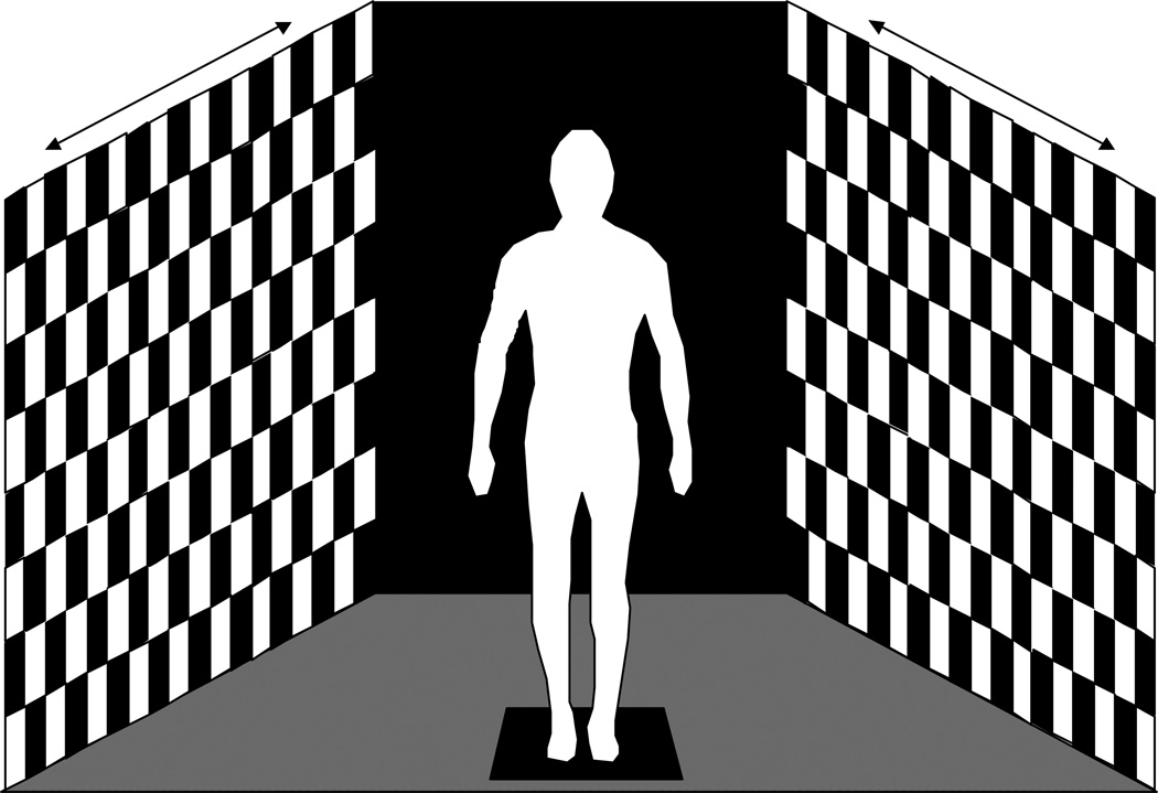
As noted in the Introduction, subjects may not always have a postural sway response at the same frequency as the sensory stimulus. Consequently, the technique was applied to postural sway data collected from human subjects as they viewed optic flow stimuli in a full field of view (180 deg horizontal, 70 deg vertical) immersive environment (Figure 1). Optic flow consisted of alternating black and white squares (15 cm x 15 cm) that moved sinusoidally in the anterior-posterior direction. Trials were conducted at stimulus frequencies of 0.1 and 0.25 Hz. In all cases, the amplitude of the movement was 16 cm peak-to-peak, and movement occurred for 90 seconds.

Figure 1.

Experimental set-up of optic flow conditions in which subject is standing in an immersive environment that encompasses a field of view of 180 degrees horizontally and 70 deg vertically. The movement of the optic flow is in the anterior-posterior direction.

Twenty healthy young subjects (9 male and 11 female, mean age = 24 years, range 21 to 30) participated after providing informed consent. They were instrumented with 6-degree of freedom electromagnetic sensors (Polhemus Fastrak) placed on top of their head and around their waist. All data were digitized at 5 Hz and stored for subsequent analysis. While viewing the moving scenes, subjects were instructed to stand in a relaxed manner, looking straight ahead, with their arms crossed in front of their chest.

Data Analysis

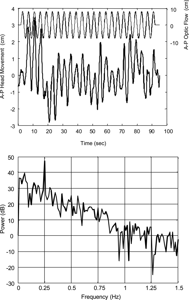
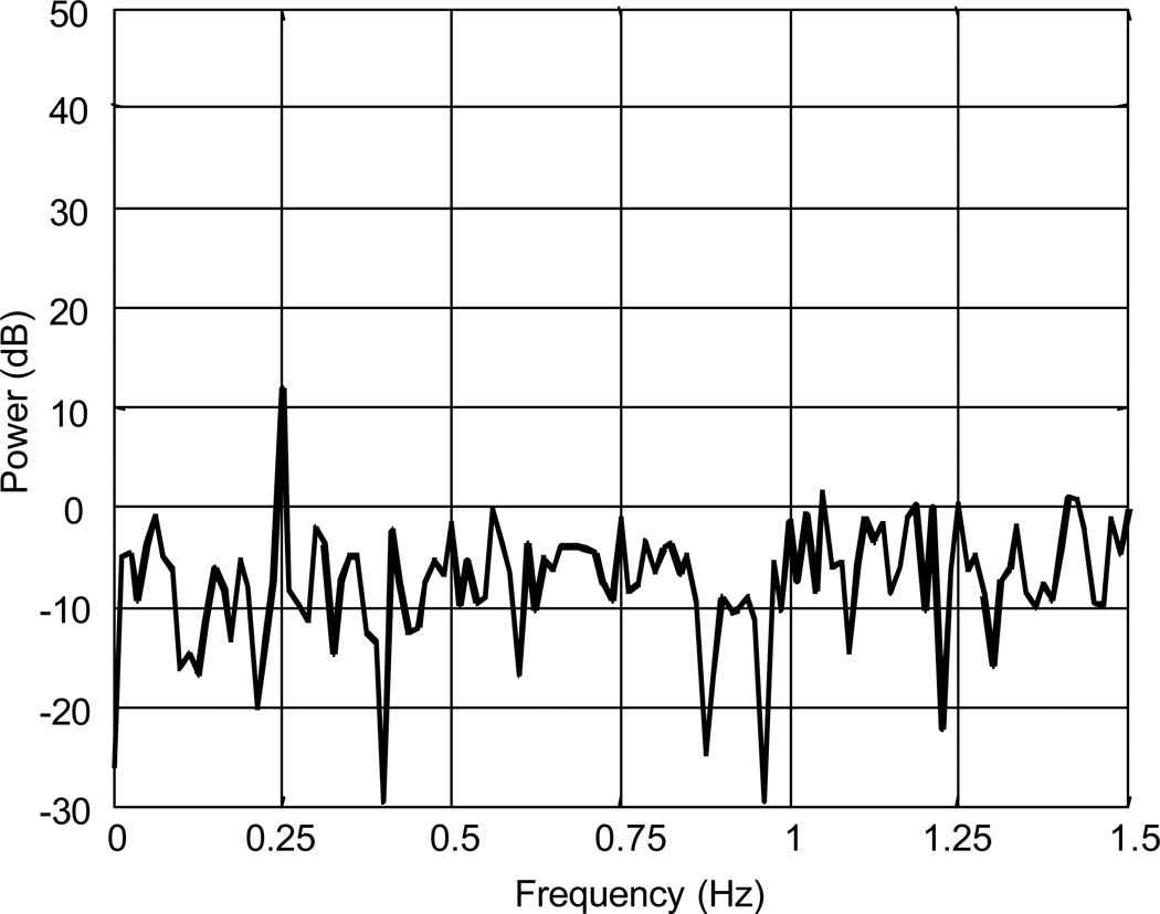
The first and last 5 seconds of the trial were discarded. After applying a digital lowpass filter (Butterworth, order 4, zero phase, cutoff frequency 2.0 Hz), periodograms (window length = 400, rectangular window, no overlap) of the data were examined. For example, postural sway data obtained from a subject while viewing a peripheral optic flow stimulus moving at 0.25 Hz is presented in Figure 2. The time series demonstrates a strong response at the stimulus frequency, although the amplitude is quite variable. In the power spectrum, a peak at 0.25 Hz can clearly be seen approximately 20 dB above the floor of the noise. However, there is a 50 dB rolloff in signal power from 0 to 1.5 Hz. Because the spectrum cannot be assumed to be zero-mean Gaussian white noise, the signal must be conditioned in some way prior to applying the statistical test. Therefore, a pre-whitening filter was applied to the data (See Appendix). Figure 3 demonstrates the spectrum of optic flow sway data after the pre-whitening filter was applied to the data in Figure 2. Observe the flatness of the spectrum, which can now be modeled as zero-mean white noise. Furthermore, the peak at 0.25 Hz is preserved.

Figure 2.

Anterior-posterior (A-P) head translation of subject A obtained while viewing the optic flow stimulus at 0.25 Hz. Top: Time series showing head translation (thick line) and optic flow stimulus (thin line). Bottom: Periodogram of head translation, before pre-whitenting filter was applied. Observe peak at 0.25 Hz.

Figure 3.

Frequency spectrum of postural sway data shown in Figure 2 (0.25 Hz optic flow). Periodogram of postural sway data after pre-whitening filter was applied. Observe flatness of spectrum with peak at 0.25 Hz maintained.

F-statistics were then computed, using the frequency range of 0.05 – 1 Hz. These were compared to a critical value of F with α = 0.05. The number of trials that passed the threshold were counted as a function of stimulus frequency.

Results

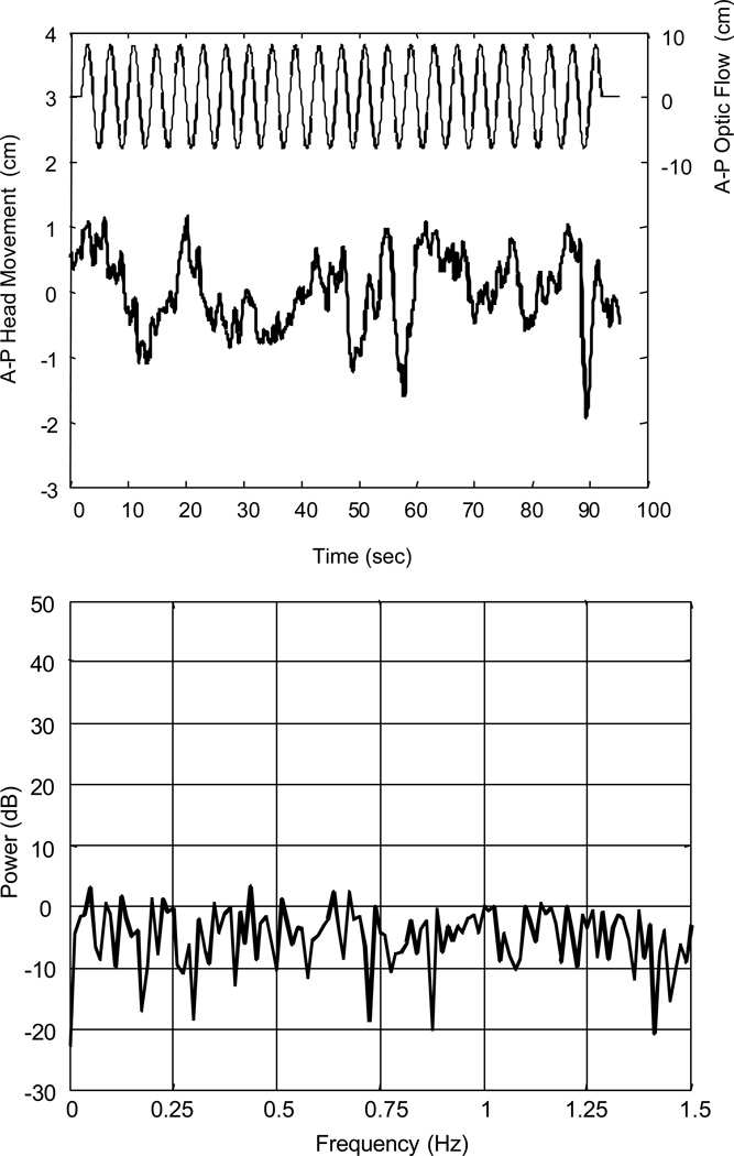
The application of this technique to data that had an obvious component at the stimulus frequency was demonstrated in Figures 2 and 3. In this example, the F-statistic was 65.6, compared to a critical F value of 3.056. In order for the method to be useful, it should also reject responses that do not appear to have a component at the stimulus frequency. Consider a different subject’s response to the same stimulus (Figure 4). The time series appears to have significant low and high frequency components, but does not have a strong response at 0.25 Hz. The pre-whitened spectrum reflects this assertion, as there is no discernible peak at 0.25 Hz. The F-statistic for this trial was 1.8, which is less than the critical F value of 3.056.

Figure 4.

Anterior-posterior (A–P) head translation of subject B obtained while viewing 0.25 Hz optic flow. Top: Time series showing head translation (thick line) and optic flow stimulus (thin line). Bottom: Periodogram of head translation, after pre-whitenting filter was applied. No observable peak at 0.25 Hz is present.

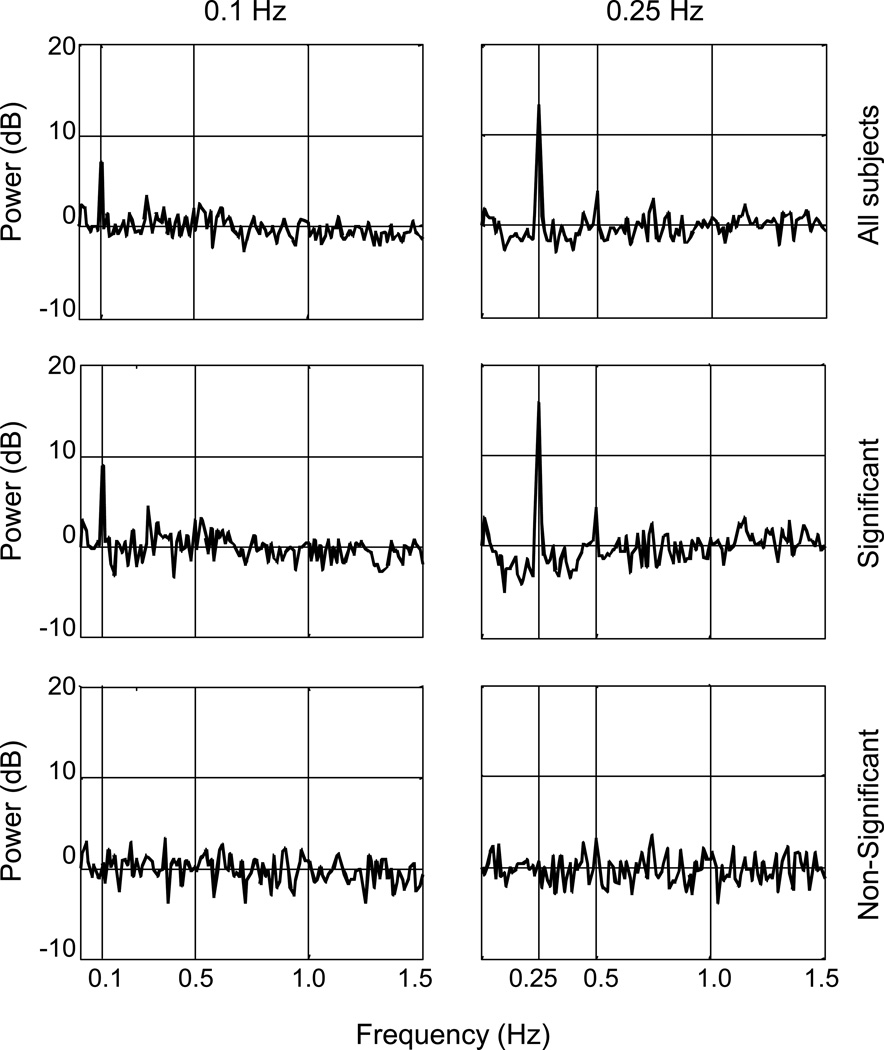
Averaged periodograms of the postural sway data (all 20 subjects) for the 2 frequency conditions are shown in Figure 5. Note how greater signal power is apparent at 0.25 Hz compared with 0.1 Hz. Twelve of the 20 subjects’ responses were significant at 0.1 Hz, and 13/20 of the responses were significant at 0.25 Hz. In addition, the average power spectra are shown for the significant and non-significant responses, demonstrating a clear difference in how subjects respond to the optic flow.

Figure 5.

Average frequency spectra of anterior-posterior head translation, as a function of frequency. Top: Average spectra for all 20 subjects. A larger peak at the stimulus frequency is seen at 0.25 Hz. Middle: Average spectra for significant responses only (n=12 at 0.1 Hz and n=13 at 0.25 Hz). Bottom: Average spectra for nonsignificant responses only (n=8 at 0.1 Hz and n=7 at 0.25 Hz).

Discussion

A reason for applying this method to postural sway data came from the authors’ observations that not all subjects responded to optic flow stimuli. This experience was corroborated by the findings of Kay and Warren,[17] who were not able to elicit visually-induced postural responses in 1/3 of their subjects. The current findings are similar, given that 15/40 (38%) of the responses were not significant. In other studies examining postural responses to visual perturbations, there have been reports of subjects not responding to all stimuli [10], and reports of excluding data from subjects who did not respond to the stimuli.[26] If a response is not detected to a perturbation of a certain sensory modality (e.g. vision), then other sensory systems may be responsible for controlling postural responses in that instance. For example, Peterka [27] has shown that for small amplitudes of optic flow stimuli, postural response gains are approximately 1, indicating a high sensitivity of the postural system to visual inputs. For greater amplitudes of optic flow stimuli, postural response gains are lower, suggesting a decrease of visual sensitivity presumably due to greater reliance on somatosensory/vestibular inputs. The proposed statistical method can help to define the conditions where individual sensory mechanisms are being used to control posture.

Consequently, fundamental questions arise regarding the use of such stimuli. 1) Is it appropriate to include response measures from data sets in which there is no apparent response to the stimulus? 2) Should the number of data sets in which a significant response was not detected be reported? 3) Can different conclusions be made if one includes non-significant responses versus not including these data? Two viewpoints can now be considered. The first assumes that all subjects are homogeneous in that they constitute a random sample of a larger population of alike individuals (healthy controls or some clinical population). All data are included in statistical analysis. A downside to this view is that inclusion of datasets in which no response is detected may prevent a significant finding from being made by minimizing differences between groups, or by increasing variability. The second view suggests that some subjects may inherently respond differently. For example, 5 of the 20 subjects did not respond to optic flow stimuli at either frequency. Immediately one may question why these subjects did not respond. Examination of these subject differences may lead to greater insight about postural control, but also may lead to less generalizability of the findings.

Of course, any number of methods can be used to detect the presence of a signal in noise.[28–30] In the postural control literature, others have used detection schema based on relative values of gain and cross-correlation function that surpass certain statistical thresholds for white noise.[19, 31]. Kay and Warren [17] considered a significant postural response to occur if the peak frequency coincided with the stimulus frequency. This method may not detect as many true significant responses, because localized peaks at higher frequencies may be smaller than the power naturally present at lower frequencies. It is for this reason that we applied a pre-whitening filter. Another method requires the computation of gain and phase over the course over several repeated trials.[22] If the gain and phase are consistent, then it can be assumed that significant responses are occurring. The tradeoff in using this method is that multiple trials need to be performed, while the method described in this paper requires only one trial per stimulus.

One of the requirements for using this technique is that the sinusoid be embedded in white noise, i.e. has a flat spectrum in the region of interest. However, postural sway data routinely demonstrates a low-pass spectrum with signal attenuation that is inversely proportional to frequency. Therefore, in order to apply this method, a pre-whitening filter was applied that flattened out the spectral response (See Appendix for details of the pre-whitening filter). The 8^th-order autoregressive model that was used to design the filter was selected because of our subjective evaluation of the whitening effect. However, we have determined that there is little difference in the resulting pre-whitened signal if one uses a 4^th, 6^th or 8^th order model. In 88% of the 40 trials, linear regression confirmed that the spectra were flat in the range from 0.05 to 1.0 Hz.

A question may arise as to how much signal power is needed in order to significantly detect a response at the stimulus frequency. Therefore, simulations were performed in order to quantify what percentage of signals with a nominal signal-to-noise ratio (SNR) would pass critical F thresholds at given values of α. Pure-tone signals (0.25 Hz) with added white noise were generated in the frequency range considered to be typical for postural sway (bandwidth 0.05 – 2.0 Hz). The amplitude of the noise was adjusted in order to achieve the desired SNR. One thousand realizations were generated for the following SNRs: 0, −3, −6, −9, −12, −15, −18, −21 dB. F-statistics were computed for each of these realizations in the range of 0.05 – 1.0 Hz, and compared with the critical F values for various values of α (0.10, 0.05, 0.025, 0.01, 0.005, 0.0025, 0.001).

The percentage of signals (60 sec duration, .05 – 1.0 Hz bandwidth) that passed the critical F values for different levels of α are tabulated as a function of the SNR for a 60 sec signal (Table 2). Given a standard α = 0.05, signals with a SNR greater than or equal to −9 dB pass all of the time. At an SNR of approximately −15 dB, 2/3 of the signals pass the critical threshold at α = 0.05 . Consequently, the test can detect relatively small signal power. If the criterion for detection was set at a more stringent level (α = 0.01), then a signal with an SNR of approximately −12 dB would pass the same amount of time. Objective criteria (such as SNR and significance level) can be used to establish what constitutes a significant postural response.

Table 2.

Percentage of simulated signals that have an F-statistic greater than the critical F-value, as a function of signal to noise ratio (SNR) and level of significance, α. 1000 realizations of a signal were generated for each SNR.

	α
SNR (dB)	0.1	0.05	0.025	0.01	0.005	0.0025	0.001
0	100	100	100	100	100	100	100
−3	100	100	100	100	100	100	100
−6	100	100	100	100	100	100	100
−9	100	100	100	99	98	98	95
−12	97	93	88	78	70	62	51
−15	75	66	57	43	32	24	18
−18	53	38	27	18	11	7	4
−21	30	18	11	6	4	3	1

Postural sway is a complex biological signal, which makes it difficult, at times, to discern if a significant response has occurred due to some stimulus. The proposed statistical-based method provides an objective rule for determining if significant postural responses occur as a result of sinusoidal sensory stimuli. Consequently, the use of such a rule could form the basis of a hypothesis test that examines if a response depends upon some experimental condition. For example, the effect of optic flow stimulus frequency on the ability to detect a significant response would have been found to be not significant using the χ² statistic. Given the widespread use of sinusoidal perturbations in the postural control literature, this method can be an important tool for understanding the sensory control of posture.

Appendix

The pre-whitening filter was constructed by fitting an 8^th order autoregressive model to the optic flow data. In the frequency domain:

$$X(f)~A{R}_p=\frac{1}{a_0+\sum _{q=1}^p{a}_q{e}^{-i2\pi fq\Delta t}}$$ (7)

Note that in order to avoid bias in the model fit due to a large component at the stimulus frequency, the components at the stimulus frequency + 1 bin were replaced by linear interpolation of the components at the neighboring frequency bins (i.e. stimulus frequency ± 2 bins). Then, the optic flow sway data were filtered using the coefficients determined from the model.

$$A(f)=a_0+\sum _{q=1}^p{a}_q{e}^{-i2\pi fq\Delta t}$$ (8)

$$X_{\mathit{\text{white}}}(f)=X(f)A(f)$$ (9)

Matlab was used to design and apply the pre-whitening filter, using the following scripts:

A=lpc1(x,p,fs,f1);  % use lpc1 to find the filter coefficients for the pre-whitening filter
                    % A is the vector of filter coefficients
                    % x is the input signal
                    % p is the order of the linear predictor
                    % fs is the sampling frequency of the input signal
                    % f1 is a vector of stimulus frequencies

y=filter(A,1,x);    % y is the pre-whitened signal

#x00025;%%%%%%%%%%%%%%%%%%%%%%%%%%%%%%%%%%%%%%%%%%%%%%%%%%%%%%%%%%%%%%%%%%%%%%

function A=lpc1(x,p,fs,f1);
         fN=fs/2;                       % fN is the Nyquist frequency
         lx=length(x);                  % Determine length of input signal
         if mod(lx,2)==1, lx=lx-1; end  % Make input signal have even number of values
         X = fft(x(1:lx),lx);           % Compute autocorrelation vector
         X2=(abs(X).^2);                % Calculate PSD of x
         LX=length(X)/2;                % Determine length of positive half of signal
         deltaf=fN/LX;                  % Determine increment in frequency
         fx = 0 : deltaf : fN-deltaf ;  % fx is the frequency vector

         % loop to get rid of peak at each stimulus frequency

         for nfreq=1:length(f1),

                  %Determine frequency bins that correspond to stimulus frequency
                  g1=find(fx==f1(nfreq));  % positive half
                  g2=lx+1-g1;              % negative half

                  % Find slope of line joining 2 points behind and ahead of stim. freq.
                  slope=(X2(g1+2)-X2(g1-2))/4;

                  % Replace the points around stim. freq. with the interpolated points
                  X2(g1-1:g1+1)= X2(g1-2)+slope*[1:3];  % positive half
                  X2(g2-1:g2+1)= X2(g2-2)-slope*[1:3];  % negative half

         end

         R = ifft(X2);                  % Return back to the time domain
         R = R./(lx-1);                 % Biased autocorrelation estimate
         [A,E] = levinson(R,p);         %Levinson-Durbin recursion to solve the normal equations
                                        that arise from the least-squares formulation

#x00025; Notes:
#x00025;  A = LPC1(X,N) finds the coefficients, A=[ 1 A(2) ... A(N+1) ],
#x00025;  of an Nth order forward linear predictor
#x00025;
#x00025;    Xp(n) = -A(2)*X(n-1) - A(3)*X(n-2) - ... - A(N+1)*X(n-N)
#x00025;
#x00025;  such that the sum of the squares of the errors
#x00025;
#x00025;    err(n) = X(n) - Xp(n)
#x00025;
#x00025;  is minimized.
#x00025;
% LPC1 uses the Levinson-Durbin recursion to solve the normal equations
% that arise from the least-squares formulation. This computation
% of the linear prediction coefficients is often referred to as the
% autocorrelation method.

References

- 1.Benson AJ, Jobson PH. Body sway induced by a low frequency alternating current. International Journal of Equilibrium Research. 1973;3:55–61. [PubMed] [Google Scholar]
- 2.Coats AC. The sinusoidal galvanic body-sway response. Acta OtoLaryngologica. 1972;74:155–162. doi: 10.3109/00016487209128436. [DOI] [PubMed] [Google Scholar]
- 3.Latt LD, Sparto PJ, Furman JM, Redfern MS. The steady-state postural response to continuous sinusoidal galvanic vestibular stimulation. Gait and Posture. 2003;18:64–72. doi: 10.1016/s0966-6362(02)00195-9. [DOI] [PubMed] [Google Scholar]
- 4.Hlavacka F, Njiokiktjien C. Postural responses evoked by sinusoidal galvanic stimulation of the labyrinth. Influence of head position. Acta Oto -Laryngologica. 1985;99:107–112. doi: 10.3109/00016488509119152. [DOI] [PubMed] [Google Scholar]
- 5.Hlavacka F, Njiokiktjien C. Sinusoidal galvanic stimulation of the labyrinths and postural responses. Physiologia Bohemoslovaca. 1986;35:63–70. [PubMed] [Google Scholar]
- 6.Storper IS, Honrubia V. Is human galvanically induced triceps surae electromyogram a vestibulospinal reflex response? Otolaryngology - Head & Neck Surgery. 1992;107:527–536. doi: 10.1177/019459989210700404. [DOI] [PubMed] [Google Scholar]
- 7.Petersen H, Magnusson M, Fransson PA, Johansson R. Vestibular disturbance at frequencies above 1 Hz affects human postural control. Acta Oto-Laryngologica. 1994;114:225–230. doi: 10.3109/00016489409126048. [DOI] [PubMed] [Google Scholar]
- 8.Berthoz A, Lacour M, Soechting JF, Vidal PP. The role of vision in the control of posture during linear motion. In: Granit R, Pompeiano O, editors. Reflex Control of Postu re and Movement (Progress in Brain Research, 50) Elsevier/North Holland Biomedical Press; 1979. pp. 197–209. [DOI] [PubMed] [Google Scholar]
- 9.Dijkstra TM, Schoner G, Giese MA, Gielen CC. Frequency dependence of the action-perception cycle for postural control in a moving visual environment: relative phase dynamics. Biological Cybernetics. 1994;71:489–501. doi: 10.1007/BF00198467. [DOI] [PubMed] [Google Scholar]
- 10.Dijkstra TM, Schoner G, Gielen CC. Temporal stability of the action-perception cycle for postural control in a moving visual environment. Experimental Brain Research. 1994;97:477–486. doi: 10.1007/BF00241542. [DOI] [PubMed] [Google Scholar]
- 11.Keshner EA. Head-trunk coordination during linear anterior-posterior translations. Journal of Neurophysiology. 2003;89:1891–1901. doi: 10.1152/jn.00836.2001. [DOI] [PubMed] [Google Scholar]
- 12.Lestienne F, Soechting J, Berthoz A. Postural readjustments induced by linear motion of visual scenes. Experimental Brain Research. 1977;28:363–384. doi: 10.1007/BF00235717. [DOI] [PubMed] [Google Scholar]
- 13.Loughlin PJ, Redfern MS, Furman JM. Time-varying characteristics of visually induced postural sway. IEEE Transactions on Rehabilitation Engineering. 1996;4:416–424. doi: 10.1109/86.547944. [DOI] [PubMed] [Google Scholar]
- 14.Loughlin PJ, Redfern MS. Spectral characteristics of visually induced postural sway in healthy elderly and healthy young subjects. IEEE Transactions on Neural Systems & Rehabilitation Engineering. 2001;9:24–30. doi: 10.1109/7333.918273. [DOI] [PubMed] [Google Scholar]
- 15.Redfern MS, Furman JM. Postural sway of patients with vestibular disorders during optic flow. Journal of Vestibular Research. 1994;4:221–230. [PubMed] [Google Scholar]
- 16.Peterka RJ, Benolken MS. Role of somatosensory and vestibular cues in attenuating visually induced human postural sway. Experimental Brain Research. 1995;105:101–110. doi: 10.1007/BF00242186. [DOI] [PubMed] [Google Scholar]
- 17.Kay BA, Warren WH., Jr Coupling of posture and gait: mode locking and parametric excitation. Biological Cybernetics. 2001;85:89–106. doi: 10.1007/PL00008002. [DOI] [PubMed] [Google Scholar]
- 18.van Asten WN, Gielen CC, van der Gon JJ. Postural movements induced by rotations of visual scenes. Journal of the Optical Society of America A-Optics & Image Science. 1988;5:1781–1789. doi: 10.1364/josaa.5.001781. [DOI] [PubMed] [Google Scholar]
- 19.van Asten WN, Gielen CC, Denier van der Gon JJ. Postural adjustments induced by simulated motion of differently structured environments. Experimental Brain Research. 1988;73:371–383. doi: 10.1007/BF00248230. [DOI] [PubMed] [Google Scholar]
- 20.Diener HC, Dichgans J, Bruzek W, Selinka H. Stabilization of human posture during induced oscillations of the body. Experimental Brain Research. 1982;45:126–132. doi: 10.1007/BF00235771. [DOI] [PubMed] [Google Scholar]
- 21.Jeka JJ, Schoner G, Dijkstra T, Ribeiro P, Lackner JR. Coupling of fingertip somatosensory information to head and body sway. Experimental Brain Research. 1997;113:475–483. doi: 10.1007/pl00005600. [DOI] [PubMed] [Google Scholar]
- 22.Jeka J, Oie K, Schoner G, Dijkstra T, Henson E. Position and velocity coupling of postural sway to somatosensory drive. Journal of Neurophysiology. 1998;79:1661–1674. doi: 10.1152/jn.1998.79.4.1661. [DOI] [PubMed] [Google Scholar]
- 23.Buchanan JJ, Horak FB. Emergence of postural patterns as a function of vision and translation frequency. Journal of Neurophysiology. 1999;81:2325–2339. doi: 10.1152/jn.1999.81.5.2325. [DOI] [PubMed] [Google Scholar]
- 24.Oie KS, Kiemel T, Jeka JJ. Multisensory fusion: simultaneous re-weighting of vision and touch for the control of human posture. Cognitive Brain Research. 2002;14:164–176. doi: 10.1016/s0926-6410(02)00071-x. [DOI] [PubMed] [Google Scholar]
- 25.Percival DB. Spectral Analysis of Univariate and Bivariate Time Series. In: Stanford JL, Vardeman SB, editors. Statistical Methods for Physical Science. New York: Academic Press; 1994. pp. 313–348. [Google Scholar]
- 26.Delorme A, Martin C. Roles of retinal periphery and depth periphery in linear vection and visual control of standing in humans. Canadian Journal of Psychology. 1986;40:176–187. doi: 10.1037/h0080091. [DOI] [PubMed] [Google Scholar]
- 27.Peterka RJ. Sensorimotor integration in human postural control. Journal of Neurophysiology. 2002;88:1097–1118. doi: 10.1152/jn.2002.88.3.1097. [DOI] [PubMed] [Google Scholar]
- 28.McDonough RN, Whalen AD. Detection of Signals in Noise. 2nd ed. San Diego: Academic Press; 1995. [Google Scholar]
- 29.Jenkins GM, Watts DG. Spectral Analysis and Its Applications. San Francisco: Holden-Day; 1968. [Google Scholar]
- 30.Koopmans LH. The Spectral Analysis of Time Series. San Diego: Academic Press; 1995. [Google Scholar]
- 31.Bertenthal BI, Rose JL, Bai DL. Perception-action coupling in the development of visual control of posture. Journal of Experimental Psychology: Human Perception & Performance. 1997;23:1631–1643. doi: 10.1037//0096-1523.23.6.1631. [DOI] [PubMed] [Google Scholar]