A Generic Path Algorithm for Regularized Statistical Estimation

Abstract

Regularization is widely used in statistics and machine learning to prevent overfitting and gear solution towards prior information. In general, a regularized estimation problem minimizes the sum of a loss function and a penalty term. The penalty term is usually weighted by a tuning parameter and encourages certain constraints on the parameters to be estimated. Particular choices of constraints lead to the popular lasso, fused-lasso, and other generalized ℓ₁ penalized regression methods. In this article we follow a recent idea by Wu (2011, 2012) and propose an exact path solver based on ordinary differential equations (EPSODE) that works for any convex loss function and can deal with generalized ℓ₁ penalties as well as more complicated regularization such as inequality constraints encountered in shape-restricted regressions and nonparametric density estimation. Non-asymptotic error bounds for the equality regularized estimates are derived. In practice, the EPSODE can be coupled with AIC, BIC, C_p or cross-validation to select an optimal tuning parameter, or provides a convenient model space for performing model averaging or aggregation. Our applications to generalized ℓ₁ regularized generalized linear models, shape-restricted regressions, Gaussian graphical models, and nonparametric density estimation showcase the potential of the EPSODE algorithm.

1 INTRODUCTION

In this article, we consider a general regularization framework

$$\underset{\mathit{\beta }\in ℝp}{min}f(\mathit{\beta })+\rho {\Vert \mathit{V}\mathit{\beta }-\mathit{d}\Vert }_1+\rho {\Vert \mathit{W}\mathit{\beta }-\mathit{e}\Vert }_{+},$$ (1)

for which we propose an efficient exact path solver based on ordinary differential equations (EPSODE). Here f : ℝ^p ↦ ℝ is a convex, smooth function of β ∈ ℝ^p, where p > 0 is the dimensionality of the parameters. For any vector v = (v_i), ||v||₁ = Σ_i |v_i| denotes its ℓ₁ norm and ||v||₊ = Σ_i max{v_i, 0} is the sum of positive parts of its components. ρ is the regularization tuning parameter and the two regularization terms embodied by the constant matrices (V, W) and vectors (d, e) enforce equality and inequality constraints among the parameters respectively as explained below. The EPSODE provides the exact solution path to (1) as the tuning parameter ρ varies.

1.1 Generality of (1)

The generality of (1) is two-fold. First, f can by any convex loss or other types of objective functions. For example, it can be the negative log-likelihood function of GLMs, negative quasi-likelihood, the exponential loss function of the AdaBoost (Friedman et al., 2000), or many other frequently used loss functions in statistics and machine learning. Second, we allow V and W to be any regularization matrices of p columns. This leads to broad applications. In particular, the first regularization term ρ||Vβ − d||₁ encourages equality constraints Vβ = d. When ρ is large enough, the minimizer β(ρ) of (1) satisfies Vβ(ρ) = d. For instance, when V is the identity matrix and d = 0, it recovers the well-known lasso regression (Tibshirani, 1996; Donoho and Johnstone, 1994) which encourages sparsity of the estimates. When

$$\mathit{V}=\left(\begin{array}{cccc}-1& 1& & \\ & \ddots & \ddots & \\ & & -1& 1\end{array}\right)$$

and d = 0, it corresponds to the fused-lasso penalty (Tibshirani et al., 2005), which leads to smoothness among neighboring regression coefficients. As we will show later, more complicated equality constraints can be incorporated with properly designed V and d. On the other hand, the second regularization term ρ||Wβ − e||₊ enforces regularization by inequality relations among regression coefficients. For large enough ρ, the minimizer β(ρ) satisfies Wβ(ρ) ≤ e. For instance, setting W as the negative identity matrix and e = 0 encourages nonnegativity of the estimates, as required in nonnegative least squares problems (Lawson and Hanson, 1987). In the isotonic regression (Robertson et al., 1988; Silvapulle and Sen, 2005), the estimates have to be nondecreasing. This can be achieved by the regularization matrix

$$\mathit{W}=\left(\begin{array}{cccc}1& -1& & \\ & \ddots & \ddots & \\ & & 1& -1\end{array}\right)$$

and e = 0. More complicated constraints that occur in shape-restricted regression and nonparametric regressions also can be incorporated as we demonstrate in later examples.

In certain applications, both equality and inequality regularizations are required. In that case, as shown in Section 2, at a large but finite ρ, the minimizer β(ρ) coincides with the solution to the following linearly constrained optimization problem

$$minf(\mathit{\beta })\text{subject}\text{to}\mathit{V}\mathit{\beta }=\mathit{d}\text{and}\mathit{W}\mathit{\beta }\le \mathit{e}.$$ (2)

Consequently EPSODE solves the linearly constrained estimation problem (2) as a by-product. In this case, path following commences from the unconstrained solution argmin f (β) and ends at the constrained solution to (2).

1.2 A Motivating Example

For illustration, we consider a merger and acquisition (M&A) data set studied in (Fan et al., 2013). This data set constitutes n = 1, 371 US companies with a binary response variable indicating whether the company becomes a leveraged buyout (LBO) target (y_i = 1) or not (y_i = 0). Seven covariates (1. cash flow, 2. cash, 3. long term investment, 4. market to book ratio, 5. log market equity, 6. tax, 7. return on S&P 500 index) are recorded for each company. There have been intensive studies on the effects of these factors on the probability of a company being a target for strategic mergers. Exploratory analysis using linear logistic regression shows no significance in most covariates.

To explore the possibly nonlinear effects of these quantitative covariates, the varying-coefficient model (Hastie and Tibshirani, 1993) can be adopted here. We discretize each predictor into, say, 10 bins and fit a logistic regression. The first bin of each predictor is used as the reference level and effect coding is applied to each discretized covariate. The circles (○) in Figure 1 denote the estimated coefficients for each bin of each predictor and hint at some interesting nonlinear effects. For instance, the chance of being an LBO target seems to monotonically decease with market-to-book ratio and be quadratic as a function of log market equity. Regularization can be utilized to borrow strength between neighboring bins and gear solution towards clearer patterns. To illustrate the flexibility of the regularization scheme (1), we apply cubic trend filtering to 5 covariates (cash flow, cash, long term investment, tax, return on S&P 500 index), impose the monotonicity (non-increasing) constraint on the ‘market-to-book ratio’ covariate, and enforce the concavity constraint on the ‘log market equity’ covariate. This can be achieved by minimizing a regularized negative logistic log-likelihood of form

Figure 1.

Snapshots of the path solution to the regularized logistic regression on the M&A data set.

$$-\ell ({\mathit{\beta }}_1,\dots ,{\mathit{\beta }}_7)+\rho \sum _{j\ne 4,5}{\Vert {\mathit{V}}_j{\mathit{\beta }}_j\Vert }_1+\rho \sum _{j=4,5}{\Vert {\mathit{W}}_j{\mathit{\beta }}_j\Vert }_{+},$$

where β_j is the vector of regression coefficients for the j-th discretized covariate. The matrices in the regularization terms are specified as

$$\begin{array}{l}{\mathit{V}}_j=\left(\begin{array}{cccccccc}-1& 2& -1& & & & & \\ & 1& -4& 6& -4& 1& & \\ & & \ddots & \ddots & \ddots & \ddots & & \\ & & 1& -4& 6& -4& 1& \\ & & & & & -1& 2& -1\end{array}\right)\text{for}j=1,2,3,6,7,\\ {\mathit{W}}_4=\left(\begin{array}{cccc}-1& 1& & \\ & \ddots & \ddots & \\ & & -1& 1\end{array}\right),\text{and}{\mathit{W}}_5=\left(\begin{array}{ccccc}1& -2& 1& & \\ & \ddots & \ddots & \ddots & \\ & & 1& -2& 1\end{array}\right).\end{array}$$

The equality constraint regularization matrix V_j, j = 1, 2, 3, 6, 7, penalizes the fourth order finite differences between the bin estimates. Thus, as ρ increases, the coefficient vectors of covariates 1–3,6–7 tend to be piecewise cubic with two ends being linear, mimicking the natural cubic spline. This is one example of the polynomial trend filtering (Kim et al., 2009; Tibshirani and Taylor, 2011). Similar to semi-parametric regressions, regularizations in polynomial trend filtering ‘let the data speak for themselves’. In contrast, the bandwidth selection in semi-parametric regressions is replaced by parameter tuning in regularizations. The number and locations of knots are automatically determined by tuning parameter which is chosen according to model selection criteria. In a similar fashion, the coefficient vector gradually becomes monotone for covariate ‘market-to-book ratio’ and concave for covariate ‘log market equity’. In addition, with ρ large enough, we recover the corresponding constrained solution, which are shown by the crosses (+) on solid lines in Figure 1. As noted above, our exact path algorithm delivers the whole solution path bridging from the unconstrained estimates (denoted by ○) to the constrained estimates (denoted by +). For example, the dotted lines in Figure 1 is a snapshot of the solution at ρ = 0.6539. Availability of the whole solution path renders model selection along the path easy. For instance the regularization parameter ρ can be chosen by minimizing the cross-validation error or other model selection criteria such as AIC, BIC, or C_p. Figure 2 displays the solution path and the AIC and BIC along the path. It shows that both criteria favor the fully regularized solution, namely the constrained estimates. The whole solution path is obtained within seconds on a laptop using a Matlab implementation of EPSODE.

Figure 2.

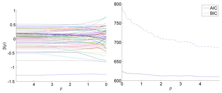
Solution and AIC/BIC paths of the regularized logistic regression on the M&A data set.

The patterns revealed by the regularized estimates match some existing finance theories. For instance, a company with low cash flow is unlikely to be an LBO target because low cash flow is hard to meet the heavy debt burden associated with the LBO. On the other hand, company carrying a high cash flow is likely to possess a new technology. It is risky to acquire such firms because it is hard to predict their profitability. The tax reason is obvious from the regularized estimates. The more tax the company is paying, the more tax benefits from an LBO. Log of market equity is a measure of company size. Smaller companies are unpredictable in their profitability and extremely large companies are unlikely to be an LBO target because LBOs are typically financed with a large proportion of external debts.

This illustrative example demonstrates the flexibility of our novel path algorithm. First, it can be applied to any convex loss function. In this example, the loss function is the negative log-likelihood of a logistic model. Second, it works for complicated regularizations like polynomial trend filtering (equality constraints), monotonicity constraint, and concavity constraint. More applications will be presented in Section 7 to illustrate the potential of EPSODE.

1.3 Previous Work and Our Contributions

Path algorithms have been devised for some special cases of the general regularization problem (1). Most notably the homotopy method (Osborne et al., 2000) and the least angle regression (LARS) procedure (Efron et al., 2004) handle lasso penalized least squares problem. The solution path generated is piecewise linear and illustrates the tradeoffs between goodness of fit and sparsity. Rosset and Zhu (2007) give sufficient conditions for a solution path to be piecewise linear and expand its applications to a wider range of loss and penalty functions. Recently Tibshirani and Taylor (2011) devise a dual path algorithm for generalized ℓ₁ penalized least squares problems, which is problem (1) with f quadratic but without the second inequality regularization term. Zhou and Lange (2013) consider (1) in full generality for quadratic f. All these work concerns regularized linear regression for which the solution path is piecewise linear. Several attempts have been made to path following for regularized GLMs for which the solution path is no longer piecewise linear. Park and Hastie (2007) propose a predictor-corrector approach to approximate the lasso path for GLMs. Friedman (2008) derives an approximate path algorithm for any convex loss regularized by a separable, but not necessarily convex penalty. Here a penalty function is called separable if its Hessian matrix is diagonal.

In two pioneering papers, Wu (2011, 2012) presents an ODE-based LARS path algorithm for GLMs, quasi-likelihoods, and Cox model, a modification of which is able to deliver the exact path for lasso solution path. The ODE approach naturally fits problems with piecewise smooth solution paths and is the strategy we adopt in this paper. Unfortunately the separability restriction on the penalty term in (Friedman, 2008; Wu, 2011, 2012) excludes many important problems encountered in real applications.

Our proposed approach generalizes previous work in several aspects. First, it works for any convex loss (or criterion) function. Second, it allows for any type of regularization in terms of linear functions of parameters, equality or inequality. Equality constrained regularizations include lasso, fused-lasso and generalized ℓ₁ penalty for example. Inequality constrained regularizations are required in shape-restricted regression and nonparametric log-concave density estimation. Last but not least, it is an exact path algorithm. Availability of the exact solution path has certain appealing virtues to statisticians. Compared to individual optimizations over a pre-specified grid of tuning parameter values, it gives a more complete picture, capturing all model changes along the path. Moreover, it greatly eases some adaptive estimation procedure based on regularization path. For instance, Bayesian model averaging over the ℓ₁ regularization path has been shown to generate superior prediction, classification and model selection performances (Ghosh and Yuan, 2009; Fraley and Percival, 2010). In each MCMC iteration, a new model on regularization path is proposed and the associated (approximate) model likelihood needs to be evaluated. The exact solution path is certainly welcome here as regularized model at any ρ is likely to be sampled.

The rest of the paper is organized as follows. Section 2 reviews the exact penalty method for optimization. Here the connections between constrained optimization and regularization in statistics are made clear. Section 3 derives in detail the EPSODE algorithm for strictly convex loss function f. Its implementation via the sweep operator and ordinary differential equations are described in Section 4. An extension of EPSODE for f convex but not necessarily strictly convex is discussed in Section 5. Non-asymptotic error bounds for equality regularized estimates are derived in Section 6. Section 7 presents various applications of EPSODE. Finally, Section 8 discusses the limitations of the path algorithm and hints at future generalizations.

2 EXACT PENALTY METHOD FOR CONVEX CONSTRAINED OPTIMIZATION

Consider the convex program

$$minf(\mathit{x})\text{subject}\text{to}{g}_i(\mathit{x})=0,1\le i\le r,\text{and}{h}_j(\mathit{x})\le 0,1\le j\le s,$$ (3)

where the objective function f is convex, equality constraint functions g_i are affine, and the inequality constraint functions h_j are convex. We further assume that f and h _j are smooth. Specifically we require that f and h _j are continuously twice differentiable. To fix notation, differential d f(x) is the row vector of partial derivatives of f at x and the gradient ∇f (x) is the transpose of d f(x). The Hessian matrix of f(·) is denoted by d²f(x).

Exact penalty method minimizes the function

$${\mathcal{E}}_{\rho }(\mathit{x})=f(\mathit{x})+\rho \sum _{i=1}^r\mid g_i(\mathit{x})\mid +\rho \sum _{j=1}^{s}max\{0,h_j(\mathit{x})\}$$ (4)

for ρ ≥ 0. Classical results (Ruszczyński, 2006, Theorems 6.9 and 7.21) state that for ρ large enough, the solution to the optimization problem (4) coincides with the solution to the original constrained convex program (3). This justifies the exact penalty method as one way to solve constrained optimization problems.

According to convex calculus (Ruszczyński, 2006, Theorem 3.5), the optimal point x(ρ) of the function (x) is characterized by the necessary and sufficient condition

$$\mathbf{0}=\nabla f(\mathit{x})+\rho \sum _{i=1}^r{s}_i\nabla g_i(\mathit{x})+\rho \sum _{j=1}^s{t}_j\nabla h_j(\mathit{x})$$ (5)

with coefficients satisfying

$$s_i\in \{\begin{array}{ll}\{-1\}\hfill & g_i(\mathit{x})<0\hfill \\ [-1,1]\hfill & g_i(\mathit{x})=0\hfill \\ \{1\}\hfill & g_i(\mathit{x})>0\hfill \end{array},\text{and}{s}_i\in \{\begin{array}{ll}\{0\}\hfill & h_j(\mathit{x})<0\hfill \\ [0,1]\hfill & h_j(\mathit{x})=0\hfill \\ \{1\}\hfill & h_j(\mathit{x})>0\hfill \end{array}.$$ (6)

The sets defining possible values of s_i and t_j are the subdifferentials of the functions |x| and x₊ = max{x, 0}. For path following to make sense, we require uniqueness and continuity of the solution x(ρ) to (4) as ρ varies. The following lemma concerns the continuity of the solution path and is the foundation of our path algorithm.

Lemma 2.1

1. (Uniqueness) If is strictly convex, then its minimizer x(ρ) is unique.

2. (Continuity) If is strictly convex and coercive over an open neighborhood of ρ, i.e., {x : (x) ≤ (z)} is compact for all z, then the minimizer x(ρ) is continuous at ρ.

3. (Continuity of s_i and t_j) Furthermore, if the gradients {∇g_i(x) : g_i(x) = 0} ∪ {∇h_j(x) : h_j(x) = 0} of active constraints are linearly independent at the solution x(ρ) over an open neighborhood of ρ, then the coefficient paths s_i(ρ) and t_j(ρ) are unique and continuous at ρ.

We remark that strict convexity only gives an easy-to-check sufficient condition for uniqueness and continuity; it is not necessary. A convex but not strictly convex function can still have a unique minimum. The absolute value function |x| offers such an example. When the loss function f is strictly convex, then is strictly convex for all ρ ≥ 0 and by Lemma 2.1 there exists a unique, continuous solution path {x(ρ) : ρ ≥ 0}. In Section 3 and 4, we derive the path algorithm assuming that f is strictly convex. When f is convex but not strictly convex, e.g., when n < p in the least squares problems, the solutions at smaller ρ may not be unique. In that case, it is still possible to obtain a solution path over the region of large ρ where the minimum of is unique. In Section 5, we extend EPSODE to the case f is convex but may not be strictly convex. The third statement of Lemma 2.1 implies that the active constraints (g_i(x) = 0 or h_j(x) = 0) with interior coefficients must stay active until the coefficients hit the end points of the permissible range, which in turn implies that the solution path is piecewise smooth. This allows us to develop a path following algorithm based on ODE.

3 THE PATH FOLLOWING ALGORITHM

In this article, we specialize to the case where the constraint functions g_i and h_j are affine, i.e., the gradient vectors ∇g_i(x) and ∇h_j(x) are constant. This leads to the regularized optimization problem formulated as (1) by defining g_i and h_j as constraint residuals $g_i(\mathit{x})={\mathit{v}}_i^t\mathit{x}-d_i$ and $h_j(\mathit{x})={\mathit{w}}_j^t\mathit{x}-e_j$. In principle a similar path algorithm can be developed for the general convex program where the inequality constraint functions h_j are relaxed to be convex. But that is beyond the scope of the current paper. In Sections 3 and 4, we assume that the loss function f is strictly convex. This assumption is relaxed in Section 5.

EPSODE works in a segment-by-segment fashion. Along the path we keep track of the following index sets determined by signs of constraint residuals

$$\begin{array}{ll}{\mathcal{N}}_{\mathrm{E}}=\{i:g_i(\mathit{x})={\mathit{v}}_i^t\mathit{x}-d_i<0\},\hfill & {\mathcal{N}}_{\mathrm{I}}=\{j:h_j(\mathit{x})={\mathit{w}}_j^t\mathit{x}-e_j<0\}\hfill \\ {\mathcal{Z}}_{\mathrm{E}}=\{i:g_i(\mathit{x})={\mathit{v}}_i^t\mathit{x}-d_i=0\},\hfill & {\mathcal{Z}}_{\mathrm{I}}=\{j:h_j(\mathit{x})={\mathit{w}}_j^t\mathit{x}-e_j=0\}\hfill \\ {\mathcal{P}}_{\mathrm{E}}=\{i:g_i(\mathit{x})={\mathit{v}}_i^t\mathit{x}-d_i>0\},\hfill & {\mathcal{P}}_{\mathrm{I}}=\{j:h_j(\mathit{x})={\mathit{w}}_j^t\mathit{x}-e_j>0\}.\hfill \end{array}$$ (7)

Along each segment of the path, the set configuration is fixed. This is implied by the continuity of both the solution and coefficient paths established in Lemma 2.1. Throughout this article, we call the constraints in or active and others inactive.

Next we derive the ODE for the solution x(ρ) on a fixed segment. Suppose we are in the interior of a segment. Let x(ρ) be the solution of (4) indexed by the penalty parameter ρ and x(ρ + Δρ) the solution when the penalty is increased by an infinitesimal amount Δρ > 0. Then the difference Δx(ρ) = x(ρ + Δρ) − x(ρ) should minimize the increase in optimal objective value. That is, to the second order, Δx is the solution to

$$\begin{array}{ll}{min}_{\mathrm{\Delta }\mathit{x}}\hfill & {\mathcal{E}}_{\rho +\mathrm{\Delta }\rho }(\mathit{x}+\mathrm{\Delta }\mathit{x})-{\mathcal{E}}_{\rho }(\mathit{x})\hfill \\ \hfill \approx \hfill & df(\mathit{x})·\mathrm{\Delta }\mathit{x}+\frac{1}{2}\mathrm{\Delta }{\mathit{x}}^t·d^{2}f(\mathit{x})·\mathrm{\Delta }\mathit{x}\hfill \\ \hfill & +(\rho +\mathrm{\Delta }\rho )·\left[-\sum _{i\in {\mathcal{N}}_{\mathrm{E}}}{\mathit{v}}_i+\sum _{i\in {\mathcal{P}}_{\mathrm{E}}}{\mathit{v}}_i+\sum _{i\in {\mathcal{P}}_{\mathrm{I}}}{\mathit{w}}_j\right]·\mathrm{\Delta }\mathit{x}\hfill \\ \hfill & +\mathrm{\Delta }\rho ·\left[-\sum _{i\in {\mathcal{N}}_{\mathrm{E}}}{g}_i(\mathit{x})+\sum _{i\in {\mathcal{P}}_{\mathrm{E}}}{g}_i(\mathit{x})+\sum _{i\in {\mathcal{P}}_{\mathrm{I}}}{h}_j(\mathit{x})\right]\hfill \\ \hfill \mathrm{s}.\mathrm{t}.\hfill & {\mathit{v}}_i^t·\mathrm{\Delta }\mathit{x}=0,i\in {\mathcal{Z}}_{\mathrm{E}},\text{and}{\mathit{w}}_j^t·\mathrm{\Delta }\mathit{x}=0,j\in {\mathcal{Z}}_{\mathrm{I}}.\hfill \end{array}$$ (8)

Note that the active constraints have to be kept active since the set configuration is fixed along this segment by Lemma 2.1. This is why we have these two sets of equality constraints. To ease notational burden, we define

$$\mathit{H}(\mathit{x})=d^{2}f(\mathit{x})\text{and}{\mathit{u}}_{\overline{\mathcal{Z}}}=-\sum _{i\in {\mathcal{N}}_{\mathrm{E}}}{\mathit{v}}_i+\sum _{i\in {\mathcal{P}}_{\mathrm{E}}}{\mathit{v}}_i+\sum _{j\in {\mathcal{P}}_{\mathrm{I}}}{\mathit{w}}_j.$$ (9)

This leads to the corresponding Lagrange multiplier problem

$$\left(\begin{array}{cc}\mathit{H}(\mathit{x})& {\mathit{U}}_{\mathcal{Z}}^t\\ {\mathit{U}}_{\mathcal{Z}}& \mathbf{0}\end{array}\right)\left(\begin{array}{c}\mathrm{\Delta }\mathit{x}\\ {\mathit{\lambda }}_{\mathcal{Z}}\end{array}\right)=\left(\begin{array}{c}-\nabla f(\mathit{x})-(\rho +\mathrm{\Delta }\rho ){\mathit{u}}_{\overline{\mathcal{Z}}}\\ \mathbf{0}\end{array}\right),$$

where the rows of the matrix are the constant differentials, ${\mathit{v}}_i^t$, i ∈ , and ${\mathit{w}}_j^t$, j ∈ (x), of the active constraint functions. Denoting the inverse of matrix as

$${\left(\begin{array}{cc}\mathit{H}(\mathit{x})& {\mathit{U}}_{\mathcal{Z}}^t\\ {\mathit{U}}_{\mathcal{Z}}& \mathbf{0}\end{array}\right)}^{-1}=\left(\begin{array}{cc}\mathit{P}(\mathit{x})& \mathit{Q}(\mathit{x})\\ {\mathit{Q}}^t(\mathit{x})& \mathit{R}(\mathit{x})\end{array}\right),$$

where

$$\begin{array}{l}\mathit{P}(\mathit{x})={\mathit{H}}^{-1}(\mathit{x})-{\mathit{H}}^{-1}(\mathit{x}){\mathit{U}}_{\mathcal{Z}}^t{\left[{\mathit{U}}_{\mathcal{Z}}{\mathit{H}}^{-1}(\mathit{x}){\mathit{U}}_{\mathcal{Z}}^t\right]}^{-1}{\mathit{U}}_{\mathcal{Z}}{\mathit{H}}^{-1}(\mathit{x})\\ \mathit{Q}(\mathit{x})={\mathit{H}}^{-1}(\mathit{x}){\mathit{U}}_{\mathcal{Z}}^t{\left[{\mathit{U}}_{\mathcal{Z}}{\mathit{H}}^{-1}(\mathit{x}){\mathit{U}}_{\mathcal{Z}}^t\right]}^{-1}\\ \mathit{R}(\mathit{x})=-{\left[{\mathit{U}}_{\mathcal{Z}}{\mathit{H}}^{-1}(\mathit{x}){\mathit{U}}_{\mathcal{Z}}^t(\mathit{x})\right]}^{-1},\end{array}$$ (10)

the solution of the difference vector Δx is

$$\begin{array}{l}\mathrm{\Delta }\mathit{x}=-\mathit{P}(\mathit{x})[\nabla f(\mathit{x})+(\rho +\mathrm{\Delta }\rho ){\mathit{u}}_{\overline{\mathcal{Z}}}]\\ =-\mathit{P}(\mathit{x})[\nabla f(\mathit{x})+\rho {\mathit{u}}_{\overline{\mathcal{Z}}}(\mathit{x})+\mathrm{\Delta }\rho ·{\mathit{u}}_{\overline{\mathcal{Z}}}]\\ =-\mathit{P}(\mathit{x})[-\rho {\mathit{U}}_{\mathcal{Z}}^t{\mathit{r}}_{\overline{\mathcal{Z}}}+\mathrm{\Delta }\rho ·{\mathit{u}}_{\overline{\mathcal{Z}}}].\end{array}$$

Note $\mathit{P}(\mathit{x}){\mathit{U}}_{\mathcal{Z}}^t=\mathbf{0}$. Therefore Δx = −Δρ · P(x) . This gives the direction for the infinitesimal update of solution vector x(ρ). Taking limit in Δρ leads to the following key result for developing the path algorithm.

Proposition 3.1

Within interior of a path segment with set configuration (7), the solution x(ρ) satisfies an ordinary differential equation (ODE)

$$\frac{d\mathit{x}(\rho )}{d\rho }=-\mathit{P}(\mathit{x}){\mathit{u}}_{\overline{\mathcal{Z}}}$$ (11)

where the matrix P(x) and vector are defined by (10) and (9).

Note that the right hand side of (11) is a constant vector in x when f is quadratic and g_i and h_j are affine. Thus the corresponding solution path is piecewise linear. This recovers the case studied in (Zhou and Lange, 2013). The differential equation (11) holds on the current segment until one of two types of events happens: an inactive constraint becomes active or vice versa. The first type of event is easy to detect – whenever a constraint function, g_i(x), i ∈ ∪ , or h_j(x), j ∈ ∪ , hits zero, we move that constraint to the active set or and start solving a new system of differential equations. To detect when the second type of event happens, we need to keep track of the coefficients s_i(x) and t_j(x) for active constraints. Whenever the coefficient of an active constraint hits the boundary of its permissible range in (6), the constraint has to be relaxed from being active in next segment. It turns out the coefficients for active constraints admit a simple representation in terms of current solution vector.

Proposition 3.2

On a path segment with set configuration (7), the coefficients s_i and t_j for active constraints are

$${\mathit{r}}_{\mathcal{Z}}(\rho )=\left(\begin{array}{c}{\mathit{s}}_{{\mathcal{Z}}_E}(\rho )\\ {\mathit{t}}_{{\mathcal{Z}}_I}(\rho )\end{array}\right)=-{\mathit{Q}}^t(\mathit{x})\left[\frac{1}{\rho }\nabla f(\mathit{x})+{\mathit{u}}_{\overline{\mathcal{Z}}}\right]$$ (12)

where x = x(ρ) is the solution at ρ and the matrix Q(x) is defined by (10).

Given current solution vector x(ρ), the coefficients of the active constraints are readily obtained from (12). Once a coefficient hits the end points, we move that constraint from the active set to the inactive set that matches the end point being hit. In next section, we detail the implementation of the path algorithm.

4 IMPLEMENTATION: ODE AND SWEEPING OPERATOR

Algorithm 1 summarizes EPSODE based on Propositions 3.1 and 3.2. It involves solving ODEs segment by segment and is extremely simple to implement using softwares with a reliable ODE solver such as the ode45 function in Matlab and the deSolve package (Soetaert et al., 2010) in R. There has been extensive research in applied mathematics on numerical methods for solving ODEs, notably the Runge-Kutta, Richardson extrapolation and predictor-corrector methods. Some path following algorithms developed for specific statistical problems (Park and Hastie, 2007; Friedman, 2008) turn out to be approximate methods for solving the corresponding ODE. Wu (2011) first explicitly uses ODE to derive an exact solution path for the lasso penalized GLM. The connection of path following to ODE relieves statisticians from the burden of developing specific path algorithms for a variety of regularization problems. For instance, the rich numerical resources of Matlab includes ODE solvers that control the tolerance for the accuracy of solution (10⁻⁶ by default) and alert the user when certain events such as constraint hitting and escape occur.

Algorithm 1.

EPSODE: Solution path for regularization problem (1) with strictly convex f.

Initialize ρ = 0, β(0) = argmin f (β) and its set configuration (7).

repeat

Solve ODE (11) until an inactive constraint becomes active or the coefficient (12) of an active constraint hits boundary.

Update the set configuration (7).

until = = = ∅

Any ODE solver repeatedly evaluates the derivative. Suppose the number of parameters is p. Computation of the matrix-vector multiplications in (11) and (12) has computation cost of order O(p²) + O(p| |) + O(| |³) if the inverse H⁻¹ of Hessian matrix of loss function f is readily available, where = ∪ and | | denotes its cardinality. Otherwise the computation cost is O(p³) + O(p| |) + O(| |³).

An alternative implementation avoids repeated matrix inversions by solving an ODE for the matrices P, Q and R themselves. The computations can be conveniently organized around the classical sweep and inverse sweep operators of regression analysis (Dempster, 1969; Goodnight, 1979; Jennrich, 1977; Little and Rubin, 2002; Lange, 2010). Suppose A is an m × m symmetric matrix. Sweeping on the kth diagonal entry a_kk ≠ 0 of A yields a new symmetric matrix  with entries

$$\begin{array}{l}{\widehat{a}}_{kk}=-\frac{1}{a_{kk}},{\widehat{a}}_{ik}=\frac{a_{ik}}{a_{kk}},i\ne k,\\ {\widehat{a}}_{kj}=\frac{a_{kj}}{a_{kk}},j\ne k,{\widehat{a}}_{ij}=a_{ij}-\frac{a_{ik}{a}_{kj}}{a_{kk}},i,j\ne k.\end{array}$$

These arithmetic operations can be undone by inverse sweeping on the same diagonal entry. Inverse sweeping on the kth diagonal entry sends the symmetric matrix A into the symmetric matrix Aˇ with entries

$$\begin{array}{l}{\check{a}}_{kk}=-\frac{1}{a_{kk}},{\check{a}}_{ik}=-\frac{a_{ik}}{a_{kk}},i\ne k,\\ {\check{a}}_{kj}=-\frac{a_{kj}}{a_{kk}},j\ne k,{\check{a}}_{ij}=a_{ij}-\frac{a_{ik}{a}_{kj}}{a_{kk}},i,j\ne k.\end{array}$$

Both sweeping and inverse sweeping preserve symmetry. Thus, all operations can be carried out on either the lower or upper triangle of A alone, saving both computational time and storage. When several sweeps or inverse sweeps are performed, their order is irrelevant.

At beginning (ρ = 0) of the path following, we initialize a sweeping tableau as

$$\left(\begin{array}{cc}{\mathit{H}}^{-1}(\mathit{x})& {\mathit{H}}^{-1}(\mathit{x}){\mathit{U}}^t\\ \ast & {\mathit{UH}}^{-1}(\mathit{x}){\mathit{U}}^t\end{array}\right),$$

where the matrix U ∈ ℝ^(r+s)×p holds all constraint differentials ${\mathit{v}}_i^t$ and ${\mathit{w}}_j^t$ in rows. Further sweeping of diagonal entries corresponding to the active constraints yields

$$\left(\begin{array}{ccc}\mathit{P}(\mathit{x})& \mathit{Q}(\mathit{x})& \mathit{P}(\mathit{x}){\mathit{U}}_{\overline{\mathcal{Z}}}^t\\ \ast & \mathit{R}(\mathit{x})& {\mathit{Q}}^t(\mathit{x}){\mathit{U}}_{\overline{\mathcal{Z}}}^t\\ \ast & \ast & U_{\overline{\mathcal{Z}}}\mathit{P}(\mathit{x}){\mathit{U}}_{\overline{\mathcal{Z}}}^t\end{array}\right).$$ (13)

Here we conveniently organized the columns of the swept active constraints before those of unswept ones. In practice the sweep tableau is not necessary as in (13) and it is enough to keep an indicator vector recording which columns are swept. The key elements for the path algorithm can be easily retrieved from the sweep tableau (13) as

$$\begin{array}{l}\frac{d\mathit{x}(\rho )}{d\rho }=-\mathit{P}(\mathit{x}){\mathit{U}}_{\overline{\mathcal{Z}}}^t{\mathit{r}}_{\overline{\mathcal{Z}}}\\ {\mathit{r}}_{\mathcal{Z}}(\rho )=-{\mathit{Q}}^t(\mathit{x}){\mathit{U}}_{\overline{\mathcal{Z}}}^t{\mathit{r}}_{\overline{Z}}-\frac{1}{\rho }{\mathit{Q}}^t(\mathit{x})\nabla f(\mathit{x}),\end{array}$$

where denotes the coefficient vector for the inactive constraints, with entries −1 for constraints in , 0 for constraints in , and 1 for constraints in ∪ . Therefore path following procedure only involves solving ODE for the whole sweep tableau (13) with sweeping or inverse sweeping at kinks between successive segments. For this purpose we derive the ODE for the sweep tableau (13). For a matrix function F(X): ℝ^n×q → ℝ^m×p,

$$DF(\mathit{X})=\frac{\partial \text{vec}F(\mathit{X})}{\partial {(\text{vec}\mathit{X})}^t}$$

denotes the mp×nq Jacobian matrix (Magnus and Neudecker, 1999). As a special case, Proposition 3.1 states Dx(ρ) = −P(x) where m = p = 1.

Proposition 4.1 (ODE for Sweep Tableau)

On a segment of path with fixed set configuration, the matrices P(ρ), Q(ρ) and R(ρ) satisfy the ordinary differential equations (ODE)

$$\begin{array}{l}D\mathit{P}(\rho )=[\mathit{P}(\mathit{x})\otimes \mathit{P}(\mathit{x})]·[D\mathit{H}(\mathit{x})]·\mathit{P}(\mathit{x}){\mathit{u}}_{\overline{\mathcal{Z}}}\\ D\mathit{Q}(\rho )=[{\mathit{Q}}^t(\mathit{x})\otimes \mathit{P}(\mathit{x})]·[D\mathit{H}(\mathit{x})]·\mathit{P}(\mathit{x}){\mathit{u}}_{\overline{\mathcal{Z}}}\\ D\mathit{R}(\rho )=[{\mathit{Q}}^t(\mathit{x})\otimes {\mathit{Q}}^t(\mathit{x})]·[D\mathit{H}(\mathit{x})]·\mathit{P}(\mathit{x}){\mathit{u}}_{\overline{\mathcal{Z}}}.\end{array}$$

Solving ODE for these matrices requires the p²-by-p Jacobian matrix of the Hessian matrix

$$\begin{array}{l}\mathit{H}(\mathit{x})=d^{2}f(\mathit{x}),\\ D\mathit{H}(\mathit{x})=\frac{\partial [\text{vec}\mathit{H}(\mathit{x})]}{\partial \text{vec}{(\mathit{x})}^t}=\frac{\partial \text{vec}[d{f}^2(\mathit{x})]}{\partial \text{vec}{(\mathit{x})}^t},\end{array}$$

which we provide for each example in Section 7 for convenience. When the number of parameter p is large, DH is a large matrix. However there is no need to compute and store DH and only the matrix vector multiplication DH · v for any vector v is needed. In light of the useful identity (B^t ⊗ A)vec(C) = vec(ACB), evaluating the derivative for the whole tableau only involves multiplying three matrices and incurs computational cost O(p³) + O(p²| |) + O(p| |²).

Although we have presented the path algorithm as moving from ρ = 0 to large ρ, it can be applied in either direction. Lasso and fused-lasso usually start from the constrained solution, while in presence of general equality constraints, e.g., polynomial trend filtering, and/or inequality constraints, the constrained solution is not readily available and the path algorithm must be initiated at ρ = 0.

5 EXTENSION OF EPSODE

So far we have assumed strict convexity of the loss function f. This unfortunately excludes many interesting applications, especially p > n case of the regression problems. In this section we briefly indicate an extension of EPSODE to the case f is convex but not necessarily strictly convex. In the proof of Proposition 3.1, the infinitesimal change of solution Δx is derived via minimizing the equality-constrained quadratic program (8), the solution to which requires inverse of Hessian H⁻¹ and thus strict convexity of f. Alternatively we may solve (8) via reparameterization. Let hold the active constraint vectors and Y ∈ be a null space matrix of , i.e., the columns of Y are orthogonal to the rows of . Then the infinitesimal change can be represented as Δx = YΔy for some vector Δy ∈ . Under this reparameterization, the quadratic program (8) is equivalent to

$$\underset{\mathrm{\Delta }\mathit{y}}{min}\frac{1}{2}\mathrm{\Delta }{\mathit{y}}^t[{\mathit{Y}}^t\mathit{H}(\mathit{x})\mathit{Y}]\mathrm{\Delta }\mathit{y}+[df(\mathit{x})+(\rho +\mathrm{\Delta }\rho ){\mathit{u}}_{\overline{\mathcal{Z}}}^t]\mathit{Y}·\mathrm{\Delta }\mathit{y}$$

with explicit solution

$$\mathrm{\Delta }\mathit{y}=-{[{\mathit{Y}}^t\mathit{H}(\mathit{x})\mathit{Y}]}^{-1}{\mathit{Y}}^t[\nabla f(\mathit{x})+(\rho +\mathrm{\Delta }\rho ){\mathit{u}}_{\overline{\mathcal{Z}}}].$$

Hence the infinitesimal change in x(ρ) is

$$\begin{array}{l}\mathrm{\Delta }\mathit{x}=-\mathit{Y}{[{\mathit{Y}}^t\mathit{H}(\mathit{x})\mathit{Y}]}^{-1}{\mathit{Y}}^t[\nabla f(\mathit{x})+(\rho +\mathrm{\Delta }\rho ){\mathit{u}}_{\overline{\mathcal{Z}}}]\\ =-\mathrm{\Delta }\rho ·\mathit{Y}{[{\mathit{Y}}^t\mathit{H}(\mathit{x})\mathit{Y}]}^{-1}{\mathit{Y}}^t{\mathit{u}}_{\overline{\mathcal{Z}}}].\end{array}$$

Again taking limit gives the following result in parallel to Proposition 3.1.

Proposition 5.1

Within interior of a path segment with set configuration (7), the solution x(ρ) satisfies an ordinary differential equation (ODE)

$$\frac{d\mathit{x}(\rho )}{d\rho }=-\mathit{Y}{[{\mathit{Y}}^t\mathit{H}(\mathit{x})\mathit{Y}]}^{-1}{\mathit{Y}}^t{\mathit{u}}_{\overline{\mathcal{Z}}}$$ (14)

where Y is a null space matrix of .

An advantage of (14) is that only non-singularity of the matrix Y^tH(x)Y is required which is much weaker than the non-singularity of H. The computational cost of calculating the derivative in (14) is O((p − | |)³) + O(p(p − | |)), which is more efficient than (11) when p − | | is small. However it requires the null space matrix Y, which is nonunique and may be expensive to compute. Fortunately the null space matrix Y is constant over each path segment and in practice can be calculated by QR decomposition of the active constraint matrix . At each kink either one constraint leaves or one enters . Therefore Y can be sequentially updated (Lawson and Hanson, 1987) and need not to be calculated anew for each segment. Which version of (11) and (14) to use depends on specific application. When the loss function f is not strictly convex, e.g., p > n case in regression analysis, only (14) applies.

6 STATISTICAL PROPERTIES

In this section, we derive error bounds for the regularized estimates produced by EPSODE using the regularized M-estimation framework (Negahban et al., 2012). We restrict to the equality constraint regularization

$$\underset{\mathit{\beta }\in ℝp}{min}f(\mathit{\beta })+\rho {\Vert \mathit{V}\mathit{\beta }\Vert }_1.$$

where V ∈ ℝ^r×p. The case with inequality regularization is outside the scope of this paper and will be pursued elsewhere.

Suppose the data is generated from β^* ∈ ℝ^p. Let $\mathcal{S}=\text{supp}(\mathit{V}{\mathit{\beta }}^{\ast })=\{j:{\mathit{v}}_j^t{\mathit{\beta }}^{\ast }\ne 0\}$ be the set of violated constraints, and and be the sub-matrices of V with corresponding rows in and respectively. We make two assumptions: (1) Vβ^* is s-sparse with | | = s and (2) V has full column rank, i.e., rank(V) = p. Note Assumption (2) implies that r ≥ p. Many popular regularizations with a tall regularization matrix V such as the sparse fused-lasso (Tibshirani et al., 2005) satisfies this assumption. Define spaces

$$\begin{array}{l}\mathcal{M}=\text{null}({\mathit{V}}_{{\mathcal{S}}^c}),{\mathcal{M}}^{\perp }=\text{row}({\mathit{V}}_{{\mathcal{S}}^c}),\\ \overline{\mathcal{M}}=\text{row}({\mathit{V}}_{\mathcal{S}}),{\overline{\mathcal{M}}}^{\perp }=\text{null}({\mathit{V}}_{\mathcal{S}}),\end{array}$$

and the projections

$$\begin{array}{l}{\mathit{\theta }}_{\overline{\mathcal{M}}}:={\text{Proj}}_{\overline{\mathcal{M}}}(\mathit{\theta })={\mathit{V}}_{\mathcal{S}}^t{({\mathit{V}}_{\mathcal{S}}{\mathit{V}}_{\mathcal{S}}^t)}^{+}{\mathit{V}}_{\mathcal{S}}\mathit{\theta }\\ {\mathit{\theta }}_{{\overline{\mathcal{M}}}^{\perp }}:={\text{Proj}}_{{\overline{\mathcal{M}}}^{\perp }}(\mathit{\theta })=[{\mathit{I}}_p-{\mathit{V}}_{\mathcal{S}}^t{({\mathit{V}}_{\mathcal{S}}{\mathit{V}}_{\mathcal{S}}^t)}^{+}{\mathit{V}}_{\mathcal{S}}]\mathit{\theta }\end{array}$$

of a vector θ ∈ ℝ^p onto spaces and respectively. The regularizer ||Vθ||₁ is decomposable with respect to the model space pair ( , ) in the sense that, for any β ∈ and γ ∈ , ||V(β + γ)||₁ = ||Vβ||₁ + ||Vγ||₁. Define a cone by

$$ℂ:=\left\{\mathbf{\Delta }\in {ℝ}^p:{\Vert \mathit{V}{\mathbf{\Delta }}_{{\overline{\mathcal{M}}}^{\perp }}\Vert }_1={\Vert {\mathit{V}}_{{\mathcal{S}}^c}{\mathbf{\Delta }}_{{\overline{\mathcal{M}}}^{\perp }}\Vert }_1\le 3{\Vert \mathit{V}{\mathbf{\Delta }}_{\overline{\mathcal{M}}}\Vert }_1\right\}$$ (15)

and a compatibility constant Ψ = ||Vθ||₁. Then we have the following deterministic error bounds for the discrepancy between the regularized estimate β̂(ρ) and the true parameter value β^*.

Proposition 6.1

Suppose ρ ≥ 2||V(V^tV)⁻¹∇f(β^*)||_∞ and f satisfies the restricted strong convexity on with parameter κ > 0, that is, for all Δ ∈ ,

$$f({\mathit{\beta }}^{\ast }+\mathbf{\Delta })-f({\mathit{\beta }}^{\ast })-\langle \nabla f({\mathit{\beta }}^{\ast }),\mathrm{\Delta }\rangle \ge \kappa {\Vert \mathbf{\Delta }\Vert }_2^2.$$

Then

$$\begin{array}{r}{\Vert \widehat{\mathit{\beta }}(\rho )-{\mathit{\beta }}^{\ast }\Vert }_2\le \frac{3}{2}{\kappa }^{-1}\rho \mathrm{\Psi },\\ {\Vert \mathit{V}[\widehat{\mathit{\beta }}(\rho )-{\mathit{\beta }}^{\ast }]\Vert }_1\le 6{\kappa }^{-1}\rho {\mathrm{\Psi }}^2.\end{array}$$

Now we specialize to the linear regression case y = Xβ^*+ε, where X ∈ ℝ^n×p and ε = (ε₁, …, ε_n)^t are iid mean zero random variables. The loss function under consideration is $f(\mathit{\beta })=\frac{1}{2n}{\Vert \mathit{y}-\mathit{X}\mathit{\beta }\Vert }_2^2$.

Corollary 6.2

Suppose that X satisfies the restricted eigenvalue condition

$$\frac{{\Vert \mathit{X}\mathit{\theta }\Vert }_2^2}{n}\ge \kappa {\Vert \theta \Vert }_2^2$$

for all θ ∈ and the column normalization condition ${\Vert {[\mathit{X}{({\mathit{V}}^t\mathit{V})}^{-1}{\mathit{V}}^t]}_j/\sqrt{n}\Vert }_2\le 1$ for all j = 1, …, r. With $\rho =4\sigma \sqrt{(lnr)/n}$ and the errors ε are mean-zero sub-Gaussian random variables with constant σ², then with probability at least 1 − 2/r,

$$\begin{array}{c}{\Vert \widehat{\mathit{\beta }}(\rho )-{\mathit{\beta }}^{\ast }\Vert }_2\le 6{\kappa }^{-1}\sigma \sqrt{\frac{lnr}{n}}\mathrm{\Psi }\\ {\Vert \widehat{\mathit{V}}[\mathit{\beta }(\rho )-{\mathit{\beta }}^{\ast }]\Vert }_1\le 24{\kappa }^{-1}\sigma \sqrt{\frac{lnr}{n}}{\mathrm{\Psi }}^2.\end{array}$$

Proposition 6.1 and Corollary 6.2 highlight a few differences with the corresponding error bounds for lasso regularized estimates (V = I_p) (Negahban et al., 2012).

• The number of parameter p does not play a role in the error bounds; the number of regularization terms r does.

• The compatibility constant Ψ = ||Vθ||₁ emphasizes the effect of the structure of the regularization matrix V on the error bounds. For lasso, V = I_p and $\mathrm{\Psi }={sup}_{{\Vert {\mathit{\theta }}_{\mathcal{S}}\Vert }_2\le 1}{\Vert {\mathit{\theta }}_{\mathcal{S}}\Vert }_1=\sqrt{s}$ (Negahban et al., 2012). For a general regularization matrix V, there is no analytic expression for Ψ but it can be readily computed numerically.

  The lasso error bound requires the column normalization condition on the original design matrix X; a general V imposes the same condition on the transformed matrix X(V^tV)⁻¹V^t.

7 APPLICATIONS

In this section, we collect some representative regularized or constrained estimation problems and demonstrate how they can be solved by path following. For all applications, we list the first three derivatives of the loss function f in (1). In fact, the third derivative is only needed when implementing by solving the ODE for the sweep tableau.

In applications such as regularized GLMs, the tuning parameter ρ in the regularization problem (1) is chosen by a model selection criterion such as AIC, BIC, C_p, or cross-validation. The cross validation errors can be readily computed using the solution path output by EPSODE. Yet the AIC, BIC, and C_p criteria require an estimate of the degrees of freedom of estimate β(ρ). In this article we use df(β(ρ)) = p − | ∪ | as a measure of the degrees of freedom under GLMs. It has previously been shown to be an unbiased estimate of the degrees of freedom for lasso penalized least squares (Efron et al., 2004; Zou et al., 2007), generalized lasso penalized least squares (Tibshirani and Taylor, 2011), and the least squares version of the regularized problem (1) (Zhou and Lange, 2013). Using the same degrees of freedom formula for GLMs is justified by the local approximation of GLM loglikelihood by weighted least squares (Park and Hastie, 2007).

7.1 GLMs and Quasi-Likelihoods with Generalized ℓ₁ Regularizations

The generalized linear model (GLM) deals with exponential families in which the sufficient statistics is Y and the conditional mean μ of Y completely determines its distribution. Conditional on the covariate vector x ∈ ℝ^p, the response variable y is modeled as

$$p(y\mid \mathit{x};\mathit{\beta },\sigma )\propto exp\left\{\frac{y\langle x,\mathit{\beta }\rangle -\psi (\langle \mathit{x},\mathit{\beta }\rangle )}{c(\sigma )}\right\},$$ (16)

where the scalar σ > 0 is a fixed and known scale parameter and the vector β is the parameters to be estimated. The function ψ: ℝ ↦ ℝ is the link function. When y ∈ ℝ, ψ(u) = u²/2 and c(σ) = σ², (16) is the normal regression model. When y ∈ {0, 1}, ψ(u) = ln(1 + exp(u)) and c(σ) = 1, (16) is the logistic regression model. When y ∈ , ψ(u) = exp(u), and c(σ) = 1, (16) is the Poisson regression model.

The quasi-likelihoods generalize GLM without assuming a specific distribution form of Y. Instead only a function relation between the conditional means μ_i and variances ${\sigma }_i^2,{\sigma }_i^2=V({\mu }_i)$ for some variance function V, is needed. Then the integral

$$Q(\mu ,y)={\int }_y^{\mu }\frac{y-t}{{\sigma }^{2}V(t)}dt$$

behaves like a log-likelihood function under mild conditions and is called the quasi-likelihood. The quasi-likelihood includes GLMs as special cases with appropriately chosen variance function V(·). Readers are referred to the classical text (McCullagh and Nelder, 1983, Table 9.1) for the commonly used quasi-likelihoods. By slightly abusing our notation, we assume a known link function between the conditional mean μ_i and linear predictor ${\mathit{x}}_i^T\mathit{\beta },\mu =\mu ({\mathit{x}}_i^T\mathit{\beta })$ and denote $Q_i(\mathit{\beta })=Q(\mu ({\mathit{x}}_i^T\mathit{\beta }),y_i)$. Then the quasi-likelihood with generalized ℓ₁ regularization takes the form

$$-Q(\mathit{\beta })+\rho {\Vert \mathit{V}\mathit{\beta }-\mathit{d}\Vert }_1=-{\sum }_{i=1}^n{Q}_i(\mathit{\beta })+\rho {\Vert \mathit{V}\mathit{\beta }-\mathit{d}\Vert }_1,$$ (17)

which is a special case of the general form (1). Specific choices of the regularization matrix V and constant vector d lead to lasso, fused-lasso, trend filtering, and many other applications.

For the path algorithm, we require the first two or three derivatives of the complete quasi-likelihood. Denoting η = Xβ with $\mathit{X}={({\mathit{x}}_1^t,{\mathit{x}}_2^t,\cdots ,{\mathit{x}}_n^t)}^t$, we have

$$\begin{array}{lll}\hfill \nabla Q(\mathit{\beta })& =\hfill & {[D\mathit{\mu }(\mathit{\beta })]}^t{\mathit{V}}^{-1}(\mathit{y}-\mathit{\mu })/{\sigma }^2={\mathit{X}}^t[D\mathit{\mu }(\mathit{\eta })]{\mathit{V}}^{-1}(\mathit{y}-\mathit{\mu })/{\sigma }^2,\hfill \\ \hfill \mathit{H}(\mathit{\beta })=d^{2}Q(\mathit{\beta })& =\hfill & [{(\mathit{y}-\mathit{\mu })}^t{\mathit{V}}^{-1}\otimes {\mathit{X}}^t]·D^2\mathit{\mu }(\mathit{\eta })·\mathit{X}/{\sigma }^2,\hfill \\ \hfill D\mathit{H}(\mathit{\beta })=d^{3}Q(\mathit{\beta })& =\hfill & [{\mathit{X}}^t\otimes {(\mathit{y}-\mathit{\mu })}^t{\mathit{V}}^{-1}\otimes {\mathit{X}}^t]·D^3\mathit{\mu }(\mathit{\eta })·\mathit{X}/{\sigma }^2,\hfill \end{array}$$ (18)

where V is a n-by-n diagonal matrix with diagonal entries $V(\mu ({\mathit{x}}_i^t\mathit{y}))$, Dμ(η) is a n-by-n diagonal matrix with diagonal entries ${\mu }^{\prime }({\mathit{x}}_i^t\mathit{\beta })$, D²μ(η) is a n²-by-n matrix with (n(i − 1) + i, i) entry equal to ${\mu }^{″}({\mathit{x}}_i^t\mathit{\beta })$ for i = 1, …, n and 0 otherwise, and D³μ(η) is a n³-by-n matrix with (n²(i−1)+n(i−1)+i, i) entry equal to ${\mu }^{‴}({\mathit{x}}_i^t\mathit{\beta })$ for i = 1, …, n and 0 otherwise. These formulas simplify for GLM with canonical link.

The most widely used ℓ₁ regularization is the lasso penalty which imposes sparsity on the regression coefficients. For numerical demonstration, we revisit the M&A example introduced in Section 1 without discretizing each predictor. We standardize each predictor first and consider the lasso penalized linear logistic regression model. Figure 3 shows the lasso solution path for each standardized predictor in the left panel and corresponding AIC and BIC scores in the right panel. The order at which predictors enter the model matches the more detailed patterns revealed by the varying coefficient model in Figure 1. The almost monotone effects of the predictors ‘market-to-book ratio’, ‘cash flow’, ‘cash’, and ‘tax’ can be captured by the usual linear logistic regression and these covariates are picked up by lasso first. The nonlinear effects shown in the other predictors are likely to be missed by the linear logistic regression. For instance, the quadratic effects of ‘log market equity’ shown in the regularized estimates in Figure 1 are missed by both AIC and BIC criteria.

Figure 3.

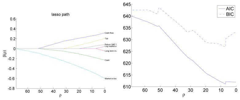
M&A example revisited. Lasso solution path on the seven standardized predictors.

7.2 Shape-Restricted Regressions

Order-constrained regression has been an important modeling tool (Robertson et al., 1988; Silva-pulle and Sen, 2005). If β denotes the parameter vector, monotone regression imposes isotone constraints β₁ ≤ β₂ ≤ · · · ≤ β_p or antitone constraints β₁ ≥ β₂ ≥ · · · ≥ β_p. In partially ordered regression, subsets of the parameters are subject to isotone or antitone constraints. In some other problems it is sensible to impose convex or concave constraints. Note that if locations of parameters are at irregularly spaced time points t₁ ≤ t₂ ≤ · · · ≤ t_p, convexity translates into the constraints

$$\frac{{\beta }_{i+2}-{\beta }_{i+1}}{t_{i+2}-t_{i+1}}\ge \frac{{\beta }_{i+1}-{\beta }_i}{t_{i+1}-t_i}$$

for 1 ≤ i ≤ p − 2. When the time intervals are uniform, the constraints simplify to β_i+2 − β_i+1 ≥ β_i+1 − β_i, i = 1, 2, · · ·, p − 1. Concavity translates into the opposite set of inequalities.

Most of previous work has focused on the linear regression problems because of the computational and theoretical complexities in the generalized linear model setting. The recent work (Rufibach, 2010) proposes an active set algorithm for GLMs with order constraints. The EPSODE algorithm conveniently provides a solution to the linearly constrained estimation problem (2). The relevant derivatives of loss function are listed in (18). It is noteworthy that EPSODE not only provides the constrained estimate but also the whole path bridging the unconstrained estimate to the constrained solution. Availability of the whole solution path renders model selection between the two extremes simple.

In the illustrative M&A example of Section 1, the bin predictors for the ‘market-to-book ratio’ are regularized by the antitone constraint and those for the ‘log market equity’ covariate by the concavity constraint.

7.3 Gaussian Graphical Models

In recent years several authors (Friedman et al., 2008; Yuan, 2008) proposed to estimate the sparse undirected graphical model by using lasso regularizations to the log-likelihood function of the precision matrix, the inverse of the variance-covariance matrix. Given an observed variance-covariance matrix Σ̂ ∈ R^p×p, the negative log-likelihood of the precision matrix Ω = Σ⁻¹ under normal assumption is

$$f(\mathbf{\Omega })=-logdet\mathbf{\Omega }+\text{tr}(\widehat{\mathbf{\sum }}\mathbf{\Omega })$$ (19)

with the MLE solution Σ̂⁻¹ when Σ̂ is non-degenerate. A zero in the precision matrix implies conditional independence of the corresponding nodes. Graphical lasso proposes to solve

$$f(\mathbf{\Omega })+\rho \sum _{i\le j}\mid {\omega }_{ij}\mid ,$$ (20)

where ρ ≥ 0 is the tuning constant and ω_ij denotes the (i, j)-element of Ω. It is well-known that the determinant function is log-concave (Magnus and Neudecker, 1999). Therefore the loss function f (19) is convex and the EPSODE algorithm applies to (20). Friedman et al. (2008) proposed an efficient coordinate descent procedure for solving (20) at a fixed ρ. A recent attempt to approximate the whole solution path is made by Yuan (2008). Again his path algorithm can be deemed as a primitive predictor-corrector method for approximating the ODE solution.

With symmetry in mind, we parameterize Ω in terms of its lower triangular part by a p(p +1)/2 column vector x and let $D\mathbf{\Omega }(\mathit{x})=\frac{\partial \text{vec}\mathbf{\Omega }}{\partial {(\text{vec}\mathit{x})}^t}$ be the corresponding p²-by-p(p + 1)/2 Jacobian matrix. Note DΩ(x) · x = vecΩ(x) and each row of DΩ(x) has exactly one nonzero entry which equals unity. We list here the first three derivatives of f.

Lemma 7.1

1. The derivatives for the Gaussian graphical model (19) with respect to Ω are

   $$\begin{array}{l}Df(\mathbf{\Omega })=df(\mathbf{\Omega })={[\mathit{vec}(-{\mathbf{\Omega }}^{-1}+\mathbf{\sum })]}^t\\ D^{2}f(\mathbf{\Omega })=d^{2}f(\mathbf{\Omega })={\mathbf{\Omega }}^{-1}\otimes {\mathbf{\Omega }}^{-1}\\ D^{3}f(\mathbf{\Omega })=-({\mathit{I}}_n\otimes {\mathit{K}}_{nn}\otimes {\mathit{I}}_n)·[{\mathbf{\Omega }}^{-1}\otimes {\mathbf{\Omega }}^{-1}\otimes \mathit{vec}({\mathbf{\Omega }}^{-1})+\mathit{vec}({\mathbf{\Omega }}^{-1})\otimes {\mathbf{\Omega }}^{-1}\otimes {\mathbf{\Omega }}^{-1}],\end{array}$$

   where K_nn is the commutation matrix (Magnus and Neudecker, 1999).

2. The derivatives for the Gaussian graphical model (19) with respect to x are

   $$\begin{array}{l}Df(\mathit{x})=Df(\mathbf{\Omega })·D\mathbf{\Omega }(\mathit{x})\\ \mathit{H}(\mathit{x})=D^{2}f(\mathit{x})={[D\mathbf{\Omega }(\mathit{x})]}^t·D^{2}f(\mathbf{\Omega })·D\mathbf{\Omega }(\mathit{x})\\ D\mathit{H}(\mathit{x})=D^{3}f(\mathit{x})=\{{[D\mathbf{\Omega }(\mathit{x})]}^t\otimes {[D\mathbf{\Omega }(\mathit{x})]}^t\}·D^{3}f(\mathbf{\Omega })·D\mathbf{\Omega }(\mathit{x}).\end{array}$$

When the covariance matrix Σ̂ is nonsingular, EPSODE can be initiated either at ρ = 0 or ρ = ∞. When Σ̂ is singular, we start from ρ = ∞ and the extended version of EPSODE (14) should be used. If starting at ρ = 0, the solution is initialized at Σ̂⁻¹; If starting at ρ = ∞, the solution is initialized at $\text{diag}({\widehat{\sigma }}_{ii}^{-1})$. Minimization of both the unpenalized and penalized objective function has to be performed over the convex cone of symmetric, positive semidefinite matrices, which is not explicitly incorporated in our path following algorithm. The next result ensures the positive definiteness of the path solution.

Lemma 7.2 (Positive definiteness along the path)

The path solution Ω(ρ) minimizes (20) over the convex cone of symmetric, positive semidefinite matrices.

We illustrate the path algorithm by the classical example of 88 students’ scores on five math courses – mechanics, vector, algebra, analysis, and statistics (Mardia et al., 1979, Table 1.2.1). Figure 4 displays the solution path from EPSODE. The top three edges chosen by lasso are analysis-algebra, statistics-algebra, and algebra-vector.

Figure 4.

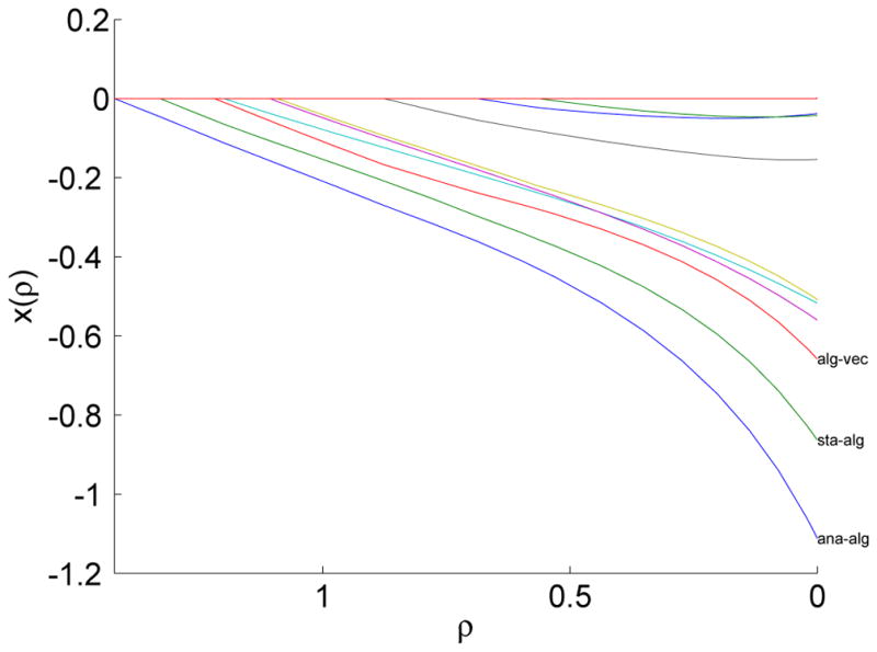
Solution path of the 10 edges in lasso-regularized Gaussian graphical model for the math score data. The top three edges chosen by lasso are labeled.

7.4 Nonparametric Density Estimation

The maximum likelihood estimation for nonparametric density estimation often involves a nontrivial, high-dimensional constrained optimization problem. In this section, we briefly demonstrate the applicability of EPSODE to the maximum likelihood estimation of univariate log-concave density. Extensions to multivariate log-concave density estimation (Cule et al., 2009, 2010) will be pursued elsewhere. It is noteworthy that, besides providing an alternative solver for log-concave density estimation, EPSODE offers the whole solution path between the unconstrained and constrained solutions. For example, an “almost” log-concave density estimate in the middle of the path can be chosen that minimizes cross-validation or prediction error. This adds another dimension to the flexibility of nonparametric modeling.

The family of log-concave densities is an attractive modeling tool. It includes most of the commonly used parametric distributions as special cases. Examples include normal, gamma with shape parameter ≥ 1, and beta densities with both parameters ≥ 1. The survey paper (Walther, 2009) gives a recent review. A probability density g(·) on ℝ is log-concave if its logarithm ϕ(x) = ln g(x) is concave. Given iid observations, from an unknown distribution of density g(·), with support at points x₁ < … < x_n with corresponding frequencies p₁, …, p_n, it is well-known (Walther, 2002) that the nonparametric MLE of g exists, is unique and takes the form ĝ = exp(ϕ̂) where ϕ̂ is continuous and piecewise linear on [x₁, x_n], with the set of knots contained in {x₁, …, x_n}, and ϕ̂ = −∞ outside the interval [x₁, x_n]. This implies that the MLE is obtained by minimizing the strictly convex function

$$f(\mathit{\varphi })=-\sum _{i=1}^n{p}_i{\varphi }_i+\sum _{k=1}^{n-1}(x_{k+1}-x_k){\int }_0^1{e}^{(1-t){\varphi }_k+t{\varphi }_{k+1}}dt.$$

over ϕ = (ϕ₁, ϕ₂, ···, ϕ_n)^t ∈ ℝⁿ subject to constraints

$$\frac{{\varphi }_{i+1}-{\varphi }_i}{x_{i+1}-x_i}\le \frac{{\varphi }_i-{\varphi }_{i-1}}{x_i-x_{i-1}},i=2,\dots ,n-1.$$

The consistency of the MLE is proved by Pal et al. (2007) and the pointwise asymptotic distribution of the MLE studied in (Balabdaoui et al., 2009).

Following Duembgen et al. (2007), we use notations

$$\begin{array}{l}{\delta }_0={\delta }_n=0,{\delta }_i=x_{i+1}-x_i,i=1,\dots ,n-1\\ J(r,s)={\int }_0^1{e}^{(1-t)r+ts}dt=\{\begin{array}{ll}\frac{e^s-e^r}{s-r}\hfill & r\ne s\hfill \\ e^r\hfill & r=s\hfill \end{array}.\end{array}$$

Then the objective function becomes

$$f(\mathit{\varphi })=-\sum _{i=1}^n{p}_i{\varphi }_i+\sum _{k=1}^{n-1}{\delta }_{k}J({\varphi }_k,{\varphi }_{k+1}).$$

The path algorithm requires up to the third derivative of the objective function f

$$\begin{array}{l}{[\nabla f(\mathit{\varphi })]}_i=-p_i+{\delta }_{i-1}{J}_{01}({\varphi }_{i-1},{\varphi }_i)+{\delta }_i{J}_{10}({\varphi }_i,{\varphi }_{i+1})\\ {[H(\mathit{\varphi })]}_{ij}={[d^{2}f(\mathit{\varphi })]}_{ij}=\{\begin{array}{ll}{\delta }_{i-1}{J}_{11}({\varphi }_{i-1},{\varphi }_i)\hfill & j=i-1\hfill \\ {\delta }_{i-1}{J}_{02}({\varphi }_{i-1},{\varphi }_i)+{\delta }_i{J}_{20}({\varphi }_i,{\varphi }_{i+1})\hfill & j=i\hfill \\ {\delta }_i{J}_{11}({\varphi }_i,{\varphi }_{i+1})\hfill & j=i+1\hfill \\ 0\hfill & \text{otherwise}\hfill \end{array}\\ \frac{\partial {[H(\mathit{\varphi })]}_{i,i-1}}{\partial {\varphi }_k}=\{\begin{array}{ll}{\delta }_{i-1}{J}_{21}({\varphi }_{i-1},{\varphi }_i)\hfill & k=i-1\hfill \\ {\delta }_{i-1}{J}_{12}({\varphi }_{i-1},{\varphi }_i)\hfill & k=i\hfill \\ 0\hfill & \text{otherwise}\hfill \end{array}\\ \frac{\partial {[H(\mathit{\varphi })]}_{i,i}}{\partial {\varphi }_k}=\{\begin{array}{ll}{\delta }_{i-1}{J}_{12}({\varphi }_{i-1},{\varphi }_i)\hfill & k=i-1\hfill \\ {\delta }_{i-1}{J}_{03}({\varphi }_{i-1},{\varphi }_i)+{\delta }_i{J}_{30}({\varphi }_i,{\varphi }_{i+1})\hfill & k=i\hfill \\ {\delta }_i{J}_{21}({\varphi }_i,{\varphi }_{i+1})\hfill & k=i+1\hfill \\ 0\hfill & \text{otherwise}\hfill \end{array}\\ \frac{\partial {[H(\mathit{\varphi })]}_{i,i+1}}{\partial {\varphi }_k}=\{\begin{array}{ll}{\delta }_i{J}_{21}({\varphi }_i,{\varphi }_{i+1})\hfill & k=i\hfill \\ {\delta }_i{J}_{12}({\varphi }_i,{\varphi }_{i+1})\hfill & k=i+1\hfill \\ 0\hfill & \text{otherwise}\hfill \end{array}.\end{array}$$

Interchanging the derivative and integral operators, justified by the dominated convergence theorem, gives a useful representation for the partial derivatives of J

$$J_{ab}(r,s)=\frac{{\partial }^{a+b}}{\partial r^a\partial s^b}J(r,s)={\int }_0^1{(1-t)}^a{t}^b{e}^{(1-t)r+ts}dt.$$

We derive a recurrence relation for J_ab(r, s) to facilitate its computation.

Lemma 7.3

J_ab(r, s) satisfy following recurrence

1. For r ≠ s,

   $$\begin{array}{l}{J}_{00}(r,s)=\frac{e^s-e^r}{s-r},J_{10}(r,s)=-\frac{e^r}{s-r}+\frac{e^s-e^r}{{(s-r)}^2}\\ J_{01}(r,s)=\frac{e^s}{s-r}-\frac{e^s-e^r}{{(s-r)}^2},J_{11}(r,s)=\frac{e^s+e^r}{{(s-r)}^2}+\frac{2(e^s-e^r)}{{(s-r)}^3}\\ J_{ab}(r,s)=\frac{a+b+s-r}{s-r}{J}_{a-1,b}(r,s)-\frac{a-1}{s-r}{J}_{a-2,b}(r,s)\\ J_{ab}(r,s)=-\frac{a+b-s+r}{s-r}{J}_{a,b-1}(r,s)+\frac{b-1}{s-r}{J}_{a,b-2}(r,s).\end{array}$$
2. For r = s,

   $$J_{ab}(r,s)=\frac{e^{r}a!b!}{(a+b+1)!}=\frac{a}{a+b+1}{J}_{a-1,b}=\frac{b}{a+b+1}{J}_{a,b-1}.$$

To illustrate the path algorithm for this problem, we simulate n = 25 points from the extremal distribution Gumbel(0,1). Figure 5 displays the constrained and unconstrained estimates of ϕ_i and the solution path bridging the two.

Figure 5.

Log-concave density estimation. n = 25 points are generated from Gumbel(0,1) distribution. Top left: Unconstrained and concavity-constrained estimates ϕ. Top right: Solution path. Bottom left: Empirical cdf and the cdf of MLE density.

7.5 Kernel Machines

In recent years kernel methods are widely used in nonlinear regression and classification problems (Scholkopf and Smola, 2001). During the review of this paper, a referee brought to our attention that various path algorithms in kernel machine methods can be unified in the ODE framework. In this section we briefly indicate this connection. Given data (y_i, x_i), i = 1, …, n,, the responses y_i ∈ ℝ are connected to the features x_i ∈ ℝ^p through a nonparametric function $h({\mathit{x}}_i)={\beta }_0+{\sum }_{j=1}^n{\beta }_{i}k({\mathit{x}}_i,{\mathit{x}}_j)$, where k: ℝ^p × ℝ^p ↦ ℝ is a positive definite kernel function and h belongs to the reproducing kernel Hilbert space . The coefficients β ∈ ℝ^p are estimated by minimizing the criterion $L(\mathit{y},h(\mathit{x}))+\rho {\Vert h\Vert }_{{\mathcal{H}}_K}^2$, where L is a loss function and ρ is the regularization parameter. Let K = [k(x_i, x _j)]_i,j ∈ ℝ^p×p be the kernel matrix based on the observed features x_i, K̃ = [1_n,K] ∈ ℝ^p×(p+1), and β̃ = [β₀, β^t]^t. This leads to the regularization problem

$${min}_{\mathit{\beta }}L(\mathit{y},{\beta }_0{\mathbf{1}}_n+\mathit{K}\mathit{\beta })+\rho {\mathit{\beta }}^t\mathit{K}\mathit{\beta }=L(\mathit{y},\stackrel{\sim }{\mathit{K}}\stackrel{\sim }{\mathit{\beta }})+\rho {\mathit{\beta }}^t\mathit{K}\mathit{\beta },$$

for which the regularization path is sought. Here are a few examples.

• The support vector machines rely on the hinge loss L(y, X) = ||1_n−diag(y)K̃β̃||₊. By switching the roles of loss and penalty, we see the criterion belongs to the EPSODE framework (1) with a quadratic β^tKβ loss and inequality regularization specified by W = −diag(y)K̃β̃ and e = −1_n. Since the Hessian of a quadratic function is constant, the path following directions (11) and (14) are constant, which leads to the piecewise linear solution path originally derived in Hastie et al. (2004). By similar arguments, the kernel quantile regression (Li et al., 2007) also admits piecewise linear solution path and allows fast computation.

• For regression with squared error loss, $L(\mathit{y},\mathit{X})={\Vert \mathit{y}-\stackrel{\sim }{\mathit{K}}\stackrel{\sim }{\mathit{\beta }}\Vert }_2^2$. At optimal solution, ${\beta }_0=\frac{1}{n}{\mathbf{1}}_n^t(\mathit{y}-\mathit{K}\mathit{\beta })$; thus it suffices to minimize ${\Vert \mathit{y}-({\mathit{I}}_n-{\mathbf{1}}_n{\mathbf{1}}_n^t)\mathit{K}\mathit{\beta }\Vert }_2^2+\rho {\mathit{\beta }}^t\mathit{K}\mathit{\beta }$ for β. This overall quadratic criterion admits an analytic solution $\widehat{\mathit{\beta }}(\rho )={[{\mathit{K}}^t({\mathit{I}}_n-{\mathbf{1}}_n{\mathbf{1}}_n^t)\mathit{K}+\rho \mathit{K}]}^{-1}{\mathit{K}}^t({\mathit{I}}_n-{\mathbf{1}}_n{\mathbf{1}}_n^t)\mathit{y}$ at each ρ. Suppose the kernel matrix K is row (column) centered and admits eigendecomposition K = UDU^t, then β̂ (ρ) = U(D² + ρD)⁻¹ DU^ty can be computed efficiently at any ρ and dismisses the need for special path following method.

• Nonlinear logistic regression uses the binomial deviance loss $L(\mathit{y},\mathit{X})={\sum }_{i=1}^n\{y_{i}h({\mathit{x}}_i)-ln(1+e^{h({\mathit{x}}_i)})\}$, with $h({\mathit{x}}_i)={\beta }_0+{\sum }_{j=1}^n{\beta }_{i}k({\mathit{x}}_i,{\mathit{x}}_j)$. Although the regularized criterion L(y, X) + ρβ^tKβ does not belong to the EPSODE formulation, the same argument as the for Proposition 3.1 shows that the path following direction is given by

  $$\left(\begin{array}{c}\frac{d{\widehat{\beta }}_0(\rho )}{d\rho }\\ \frac{d\widehat{\mathit{\beta }}(\rho )}{d\rho }\end{array}\right)=-2{[d^{2}L(\stackrel{\sim }{\mathit{\beta }})+2\rho {\stackrel{\sim }{\mathit{K}}}_0]}^{-1}\mathit{K}\left(\begin{array}{c}0\\ \widehat{\mathit{\beta }}(\rho )\end{array}\right),$$

  where K̃₀ ∈ ℝ^(p+1)×(p+1) is the original kernel matrix K augmented by an extra (first) row and (first) column of 0.

8 CONCLUSIONS

In this article we propose a generic path following algorithm EPSODE that works for any regularization problems of form (1). The advantages are its simplicity and generality. Path following only involves solving ODEs segment by segment and is simple to implement using popular softwares such as R and Matlab. Besides providing the whole regularization path, it also gives a solver for linearly constrained optimization problems that frequently arise in statistics. Our applications to shape-restricted regressions and nonparametric density estimation are special cases in particular.

Several extensions deserve further study. Current algorithm requires sufficient smoothness (twice differentiable) in the loss function. This precludes certain applications with non-smooth objective function, e.g., the Huber loss in robust estimation and the loss function in quantile regression. Generalization of our path algorithm to regularization of these loss functions requires further research. Another restriction in our formulation is the linearity in the regularization terms. In sparse regressions, several authors have proposed nonlinear and non-convex penalties. The bridge regression (Frank and Friedman, 1993) and SCAD penalties (Fan and Li, 2001) fall into this category. As observed in (Friedman, 2008), when the penalty is not convex, the solution path may not be continuous and poses difficulty in path following, which strongly depends on the continuity and smoothness of the solution path. Fortunately, in these problems, the discontinuities only occur when new variables enter or leave the model. A promising strategy is to initialize the starting point of next segment by solving an equality constrained optimization problem. This again invites further investigation. Lastly, our formulation (1) imposes same penalty parameter on equality and inequality regularization terms. Relaxing to different tuning parameters apparently increases flexibility of the regularization scheme. In this setup, the relevant target will be a “solution surface” instead of “solution path”, which is worth further investigation.

References

- Balabdaoui F, Rufibach K, Wellner JA. Limit distribution theory for maximum likelihood estimation of a log-concave density. Ann Statist. 2009;37(3):1299–1331. doi: 10.1214/08-AOS609. [DOI] [PMC free article] [PubMed] [Google Scholar]
- Cule M, Gramacy RB, Samworth R. LogConcDEAD: An R package for maximum likelihood estimation of a multivariate log-concave density. Journal of Statistical Software. 2009;29(2):1–20. [Google Scholar]
- Cule M, Samworth R, Stewart M. Maximum likelihood estimation of a multidimensional log-concave density. Journal of the Royal Statistical Society Series B. 2010;72(5):545–607. [Google Scholar]
- Dempster AP. Addison-Wesley series in behavioral sciences. Addison-Wesley; Reading, MA: 1969. Elements of Continuous Multivariate Analysis. [Google Scholar]
- Donoho DL, Johnstone IM. Ideal spatial adaptation by wavelet shrinkage. Biometrika. 1994;81(3):425–455. [Google Scholar]
- Duembgen L, Rufibach K, Huesler A. Active set and EM algorithms for log-concave densities based on complete and censored data. 2007. [Google Scholar]
- Efron B, Hastie T, Johnstone I, Tibshirani R. Least angle regression. Ann Statist. 2004;32(2):407–499. With discussion, and a rejoinder by the authors. [Google Scholar]
- Fan J, Li R. Variable selection via nonconcave penalized likelihood and its oracle properties. J Amer Statist Assoc. 2001;96(456):1348–1360. [Google Scholar]
- Fan J, Maity A, Wang Y, Wu Y. Parametrically guided generalized additive models with application to merger and acquisition data. J Nonparametr Stat. 2013;25:109–128. doi: 10.1080/10485252.2012.735233. [DOI] [PMC free article] [PubMed] [Google Scholar]
- Fraley C, Percival D. Technical Report 541. Department of Statistics, University of Washington; Seattle, WA: 2010. Model-averaged ℓ1 regularization using Markov chain monte carlo model composition. [Google Scholar]
- Frank IE, Friedman JH. A statistical view of some chemometrics regression tools. Technometrics. 1993;35(2):109–135. [Google Scholar]
- Friedman J. Fast sparse regression and classification. 2008 http://www-stat.stanford.edu/jhf/ftp/GPSpaper.pdf.
- Friedman J, Hastie T, Tibshirani R. Additive logistic regression: a statistical view of boosting. The Annals of Statistics. 2000;28(2):337–407. [Google Scholar]
- Friedman J, Hastie T, Tibshirani R. Sparse inverse covariance estimation with the graphical lasso. Biostatistics. 2008;9(3):432–441. doi: 10.1093/biostatistics/kxm045. [DOI] [PMC free article] [PubMed] [Google Scholar]
- Ghosh D, Yuan Z. An improved model averaging scheme for logistic regression. J Multivariate Anal. 2009;100(8):1670–1681. doi: 10.1016/j.jmva.2009.01.006. [DOI] [PMC free article] [PubMed] [Google Scholar]
- Goodnight JH. A tutorial on the sweep operator. Amer Statist. 1979;33(3):149–158. [Google Scholar]
- Hastie T, Rosset S, Tibshirani R, Zhu J. The entire regularization path for the support vector machine. J Mach Learn Res. 2004;5:1391–1415. [Google Scholar]
- Hastie T, Tibshirani R. Varying-coefficient models. J Roy Statist Soc Ser B. 1993;55(4):757–796. With discussion and a reply by the authors. [Google Scholar]
- Jennrich R. Statistical Methods for Digital Computers. Wiley-Interscience; New York: 1977. Stepwise regression; pp. 58–75. [Google Scholar]
- Kim SJ, Koh K, Boyd S, Gorinevsky D. l1 trend filtering. SIAM Rev. 2009;51(2):339–360. [Google Scholar]
- Lange K. Statistics and Computing. 2 Springer; New York: 2010. Numerical Analysis for Statisticians. [Google Scholar]
- Lawson CL, Hanson RJ. Classics in Applied Mathematics. Society for Industrial Mathematics; 1987. Solving Least Squares Problems. new edition edition. [Google Scholar]
- Li Y, Liu Y, Zhu J. Quantile regression in reproducing kernel Hilbert spaces. J Amer Statist Assoc. 2007;102(477):255–268. [Google Scholar]
- Little RJA, Rubin DB. Wiley Series in Probability and Statistics. 2 Wiley-Interscience [John Wiley & Sons]; Hoboken, NJ: 2002. Statistical Analysis with Missing Data. [Google Scholar]
- Magnus JR, Neudecker H. Wiley Series in Probability and Statistics. John Wiley & Sons Ltd; Chichester: 1999. Matrix Differential Calculus with Applications in Statistics and Econometrics. [Google Scholar]
- Mardia KV, Kent JT, Bibby JM. Multivariate Analysis. Academic Press [Harcourt Brace Jovanovich Publishers]; London: 1979. Probability and Mathematical Statistics: A Series of Monographs and Textbooks. [Google Scholar]
- McCullagh P, Nelder JA. Monographs on Statistics and Applied Probability. Chapman & Hall; London: 1983. Generalized Linear Models. [Google Scholar]
- Negahban S, Ravikumar PD, Wainwright MJ, Yu B. A unified framework for high-dimensional analysis of m-estimators with decomposable regularizers. Statistical Science. 2012;27:538–557. [Google Scholar]
- Osborne MR, Presnell B, Turlach BA. A new approach to variable selection in least squares problems. IMA J Numer Anal. 2000;20(3):389–403. [Google Scholar]
- Pal JK, Woodroofe M, Meyer M. Complex datasets and inverse problems, volume 54 of IMS Lecture Notes Monogr Ser. Inst. Math. Statist; Beachwood, OH: 2007. Estimating a Polya frequency function2; pp. 239–249. [Google Scholar]
- Park MY, Hastie T. L1-regularization path algorithm for generalized linear models. J R Stat Soc Ser B Stat Methodol. 2007;69(4):659–677. [Google Scholar]
- Robertson T, Wright FT, Dykstra RL. Wiley Series in Probability and Mathematical Statistics: Probability and Mathematical Statistics. John Wiley & Sons Ltd; Chichester: 1988. Order Restricted Statistical Inference. [Google Scholar]
- Rosset S, Zhu J. Piecewise linear regularized solution paths. Ann Statist. 2007;35(3):1012–1030. [Google Scholar]
- Rufibach K. An active set algorithm to estimate parameters in generalized linear models with ordered predictors. Computational Statistics & Data Analysis. 2010;54(6):1442–1456. [Google Scholar]
- Ruszczyński A. Nonlinear Optimization. Princeton University Press; Princeton, NJ: 2006. [Google Scholar]
- Scholkopf B, Smola AJ. Learning with Kernels: Support Vector Machines, Regularization, Optimization, and Beyond. MIT Press; Cambridge, MA, USA: 2001. [Google Scholar]
- Silvapulle MJ, Sen PK. Wiley Series in Probability and Statistics. Wiley-Interscience [John Wiley & Sons]; Hoboken, NJ: 2005. Constrained Statistical Inference: Inequality, Order, and Shape Restrictions. [Google Scholar]
- Soetaert K, Petzoldt T, Setzer RW. Solving differential equations in R: Package deSolve. Journal of Statistical Software. 2010;33(9):1–25. [Google Scholar]
- Tibshirani R. Regression shrinkage and selection via the lasso. J Roy Statist Soc Ser B. 1996;58(1):267–288. [Google Scholar]
- Tibshirani R, Saunders M, Rosset S, Zhu J, Knight K. Sparsity and smoothness via the fused lasso. J R Stat Soc Ser B Stat Methodol. 2005;67(1):91–108. [Google Scholar]
- Tibshirani RJ, Taylor J. The solution path of the generalized lasso. Ann Statist. 2011;39(3):1335–1371. [Google Scholar]
- Walther G. Detecting the presence of mixing with multiscale maximum likelihood. J Amer Statist Assoc. 2002;97(458):508–513. [Google Scholar]
- Walther G. Inference and modeling with log-concave distributions. Statist Sci. 2009;24(3):319–327. [Google Scholar]
- Wu Y. An ordinary differential equation-based solution path algorithm. Journal of Non-parametric Statistics. 2011;23:185–199. doi: 10.1080/10485252.2010.490584. [DOI] [PMC free article] [PubMed] [Google Scholar]
- Wu Y. Elastic net for Coxs proportional hazards model with a solution path algorithm. Statistical Sinica. 2012;22:271–294. doi: 10.5705/ss.2010.107. [DOI] [PMC free article] [PubMed] [Google Scholar]
- Yuan M. Efficient computation of ℓ1 regularized estimates in Gaussian graphical models. J Comput Graph Statist. 2008;17(4):809–826. [Google Scholar]
- Zhou H, Lange K. A path algorithm for constrained estimation. Journal of Computational and Graphical Statistics. 2013;22:261–283. doi: 10.1080/10618600.2012.681248. [DOI] [PMC free article] [PubMed] [Google Scholar]
- Zou H, Hastie T, Tibshirani R. On the “degrees of freedom” of the lasso. Ann Statist. 2007;35(5):2173–2192. [Google Scholar]