

Abstract
The efficient coding hypothesis posits that sensory systems maximize information transmitted to the brain about the environment. We develop a precise and testable form of this hypothesis in the context of encoding a sensory variable with a population of noisy neurons, each characterized by a tuning curve. We parameterize the population with two continuous functions that control the density and amplitude of the tuning curves, assuming that the tuning widths vary inversely with the cell density. This parameterization allows us to solve, in closed form, for the information-maximizing allocation of tuning curves as a function of the prior probability distribution of sensory variables. For the optimal population, the cell density is proportional to the prior, such that more cells with narrower tuning are allocated to encode higher probability stimuli, and that each cell transmits an equal portion of the stimulus probability mass. We also compute the stimulus discrimination capabilities of a perceptual system that relies on this neural representation, and find that the best achievable discrimination thresholds are inversely proportional to the sensory prior. We examine how the prior information that is implicitly encoded in the tuning curves of the optimal population may used for perceptual inference, and derive a novel decoder, the Bayesian population vector, that closely approximates a Bayesian least-squares estimator that has explicit access to the prior. Finally, we generalize these results to sigmoidal tuning curves, correlated neural variability, and a broader class of objective functions. These results provide a principled embedding of sensory prior information in neural populations, and yield predictions that are readily testable with environmental, physiological, and perceptual data.
1 Introduction
Many bottom-up theories of neural encoding posit that sensory systems are optimized to represent signals that occur in the natural environment of an organism (Attneave, 1954; Barlow, 1961). A precise specification of the optimality of a sensory representation requires four components: (1) the family of neural transformations (specifying the encoding of natural signals in neural activity), over which the optimum is to be taken; (2) the noise that is introduced by the neural transformations; (3) the types of signals that are to be encoded, and their prevalence in the natural environment; and (4) the metabolic costs of building, operating, and maintaining the system (Simoncelli and Olshausen, 2001). Although optimal solutions have been derived analytically for some specific choices of these components (e.g., linear response models and Gaussian signal and noise distributions (Atick and Redlich, 1990; Doi et al., 2012)), and numerical solutions have been examined for other cases (e.g., a population of linear-nonlinear neurons (Bell and Sejnowski, 1997; Karklin and Simoncelli, 2012; Tkačik et al., 2010)), the general problem is intractable.
A substantial literature has considered simple population coding models in which each neuron’s mean response to a scalar variable is characterized by a tuning curve (e.g., Jazayeri and Movshon, 2006; Ma et al., 2006; Pouget et al., 2003; Salinas and Abbott, 1994; Sanger, 1996; Seung and Sompolinsky, 1993; Snippe, 1996; Zemel et al., 1998; Zhang et al., 1998). For these models, several authors have examined the optimization of Fisher information, which expresses a bound on the mean squared error of an unbiased estimator (Brown and Bäcker, 2006; Montemurro and Panzeri, 2006; Pouget et al., 1999; Zhang and Sejnowski, 1999). In these results, the distribution of sensory variables is assumed to be uniform, and the populations are assumed to be homogeneous with regard to tuning curve shape, spacing, and amplitude.
The distribution of sensory variables encountered in the environment is often non-uniform, and it is thus of interest to understand how these variations in probability affect the design of optimal populations. It would seem natural that a neural system should devote more resources to regions of sensory space that occur with higher probability, analogous to results in coding theory (Gersho and Gray, 1991). At the single neuron level, several publications describe solutions in which monotonic neural response functions allocate greater dynamic range to more frequently occurring stimuli (Laughlin, 1981; McDonnell and Stocks, 2008; Nadal and Parga, 1994; von der Twer and MacLeod, 2001; Wang et al., 2012). At the population level, optimal non-uniform allocations of neurons with identical tuning curves have been derived for non-uniform stimulus distributions (Brunel and Nadal, 1998; Harper and McAlpine, 2004).
Here, we examine the influence of a sensory prior on the optimal allocation of neurons and spikes in a population, and the implications of this optimal allocation for subsequent perception. Given a prior distribution over a scalar stimulus parameter, and a resource budget of N neurons with an average of R spikes/sec for the entire population, we seek the optimal shapes, positions, and amplitudes of the tuning curves. We parameterize the population in terms of two continuous functions expressing the density and gain of the tuning curves. As a base case, we assume Poisson-distributed spike counts, and optimize a lower bound on mutual information based on Fisher information. We use an approximation of the Fisher information that allows us to obtain a closed form solution for the optimally efficient population, as well as a bound on subsequent perceptual discriminability. In particular, we find that the optimal density of tuning curves is directly proportional to the prior and that the best achievable discrimination thresholds are inversely proportional to the prior. We demonstrate how to test these predictions with environmental, physiological, and perceptual data.
Our results are optimized for coding efficiency, which many have argued is a reasonable task-independent objective for early stages of sensory processing, but seems unlikely to explain more specialized later stages that are responsible for producing actions (Geisler et al., 2009). Nevertheless, if we take seriously the interpretation of perception as a process of statistical inference (Helmholtz, 2000), then these later stages must rely on knowledge of the sensory prior. Although such prior information has been widely used in formulating Bayesian explanations for perceptual phenomena (Knill and Richards, 1996), the means by which it is represented within the brain is currently unknown (Simoncelli, 2009; Stocker and Simoncelli, 2006). Previous studies have either assumed that sensory priors are uniform (Jazayeri and Movshon, 2006; Zemel et al., 1998), or explicitly represented in the spiking activity of a separate population of neurons (Ma et al., 2006; Yang et al., 2012), or implicitly represented in the gains (Simoncelli, 2003), the sum (Simoncelli, 2009), or the distribution of preferred stimuli (Fischer and Peña, 2011; Girshick et al., 2011; Shi and Griffiths, 2009) of the tuning curves in the encoding population.
Our efficient coding population provides a generalization of these latter proposals, embedding prior probability structure in the distribution and shapes of tuning curves. We show how these embedded probabilities may be used in inference problems, and derive a novel decoder that extracts and uses the implicit prior to produce approximate Bayesian perceptual estimates that minimize mean squared error. We demonstrate (through simulations) that this decoder outperforms the well-known “population vector” decoder (Georgopoulos et al., 1986), which has been previously shown to approximate Bayesian estimation under strong assumptions about the encoding population (Fischer and Peña, 2011; Girshick et al., 2011; Shi and Griffiths, 2009; Wei and Stocker, 2012a). We also show that our decoder performs nearly as well as a Bayesian decoder that has explicit access to prior information. Finally, we generalize our formulation to consider a family of alternative optimality principles (which includes Fisher bounds on estimation error and discriminability as special cases), sigmoidal tuning curves, and non-Poisson correlated spiking models. Portions of this work were initially presented in (Ganguli, 2012; Ganguli and Simoncelli, 2010, 2012).
2 Efficient Sensory Coding
2.1 Encoding Model
We begin with a conventional descriptive model for a population of N neurons responding to a single scalar variable, denoted s (e.g., Jazayeri and Movshon, 2006; Ma et al., 2006; Pouget et al., 2003; Salinas and Abbott, 1994; Sanger, 1996; Seung and Sompolinsky, 1993; Snippe, 1996; Zemel et al., 1998; Zhang et al., 1998). Assume the number of spikes emitted in a given time interval by the nth neuron is a sample from an independent Poisson process, with mean rate determined by its tuning function, hn(s) (section 4.3 provides a generalization to non-Poisson correlated neuronal variability). The probability distribution of the population response can be written as:
| (1) |
We assume that the total expected spike rate, R, of the population is limited, which imposes a constraint on the tuning curves:
| (2) |
where p(s) is the probability distribution of stimuli in the environment. We refer to this as a sensory prior, in anticipation of its use in solving Bayesian inference problems based on the population response (see section 3).
2.2 Objective function
What is the best way to represent values drawn from p(s) using these N neurons, and limiting the total population response to a mean of R spikes? Intuitively, one might expect that more resources (spikes and/or neurons) should be locally allocated to stimuli that are more probable, thereby increasing the accuracy with which they are represented. But it is not obvious a priori exactly how the resources should be distributed, or whether the optimal solution is unique.
To formulate a specific objective function, we follow the efficient coding hypothesis, which asserts that early sensory systems evolved to maximize the information they convey about incoming signals, subject to metabolic constraints (Attneave, 1954; Barlow, 1961). Quantitatively, we seek the set of tuning curves that maximize the mutual information, I(r⃗; s), between the stimuli and the population responses:
| (3) |
The term H(s) is the entropy, or amount of information inherent in p(s), and is independent of the neural population.
The mutual information is notoriously difficult to compute (or maximize) as it requires summation/integration over the high-dimensional joint probability distribution of all possible stimuli and population responses. For analytical tractability, we instead choose to optimize a well-known lower bound on mutual information (Brunel and Nadal, 1998; Cover and Thomas, 1991):
| (4) |
where If (s) is the Fisher information, which can be expressed in terms of a second-order expansion of the log-likelihood function (Cox and Hinkley, 1974):
The bound of Eq. (4) is tight in the limit of low noise, which occurs as either N or R increase (Brunel and Nadal, 1998). The Fisher information quantifies the accuracy with which the population responses represent different values of the stimulus. It can also be used to place lower bounds on the mean squared error of an unbiased estimator (Cox and Hinkley, 1974), or alternatively, the discrimination performance of a (possibly biased) perceptual system (Seriès et al., 2009). We later generalize our analysis to handle a family of objective functions which includes these bounds as special cases (see section 4.1).
For the independent Poisson noise model, the Fisher information can be written as a function of the tuning curves (Seung and Sompolinsky, 1993),
| (5) |
where is the derivative of the nth tuning curve. Substituting this expression into Eq. (4) and adding the resource constraint of Eq. (2), allows us to express the full efficient coding problem as:
| (6) |
Even with the substitution of the Fisher bound, the objective function in Eq. (6) is non-convex over the high-dimensional parameter space (the full set of continuous tuning curves), making numerical optimization intractable. To proceed, we introduce a compact parameterization of the tuning curves which allows us to obtain an analytical solution.
2.3 Parameterization of a heterogeneous population
To develop a parametric model of tuning curves, we take inspiration from theoretical and experimental evidence that shows: (1) for many sensory variables, physiologically measured tuning curves exhibit significant heterogeneity in their spacings, widths and amplitudes; and (2) even if one assumes tuning curves of fixed width and amplitude, heterogeneous spacings are optimal for coding stimuli drawn from non-uniform prior distributions (Brunel and Nadal, 1998; Harper and McAlpine, 2004). We add to these observations an assumption that adjacent tuning curves in our idealized population should overlap by some fixed amount, such that they uniformly “tile” the stimulus space. The intuitive motivation is that if there is a degree of overlap that is optimal for transmitting information, this should hold regardless of the spacing between curves. In practice, constraining the tuning widths also greatly simplifies the optimization problem, allowing (as shown below) a closed-form solution. We enforce this assumption by parameterizing the population as a warped and re-scaled convolutional population (i.e., a population with identical tuning curves shifted to lie on a uniform lattice, such that the population tiles), as specified by a cell density function, d(s), and a gain function, g(s), as illustrated in Fig. 1. The tuning widths in the resulting heterogeneous population are proportional to the spacing between tuning curves, maintaining the tiling properties of the initial homogeneous population. Intuitively, d(s) and g(s) define the local allocation of the global resources N and R, respectively.
Figure 1.

Construction of a heterogeneous population of neurons. (a) Homogeneous population with Gaussian tuning curves on the unit lattice. The tuning width, σ = 0.55, is chosen so that the curves approximately tile the stimulus space. (b) The Fisher information of the convolutional population (green) is approximately constant. (c) Inset shows d(s), the tuning curve density. The cumulative integral of this function, D(s), alters the positions and widths of the tuning curves in the convolutional population. (d) The warped population, with tuning curve peaks (aligned with tick marks, at locations sn = D−1(n)), is scaled by the gain function, g(s) (blue). A single tuning curve is highlighted (red) to illustrate the effect of the warping and scaling operations. (e) The Fisher information of this heterogeneous population, which provides a bound on perceptual discriminability, is approximately proportional to d2(s)g(s).
To specify the parameterization, we first define a convolutional population of tuning curves, identical in form and evenly spaced on the unit lattice, such that they approximately tile the space:
| (7) |
The tiling property has been assumed in previous work, where it enabled the derivation of maximum likelihood decoders (Jazayeri and Movshon, 2006; Ma et al., 2006; Zemel et al., 1998). Note that this form of tiling is inconsistent with sigmoidal tuning curves, so we handle this case separately (see section 4.2). We also assume that the Fisher information of this population (Eq. (5)) is approximately constant:
| (8) |
where ϕ(s − n) is the Fisher information of the nth neuron. The value of the constant, Iconv, is dependent on the details of the tuning curve shape, h(s), which we leave unspecified. As an example, Fig. 1(a–b) shows through numerical simulation that a convolutional population of Gaussian tuning curves, with appropriate width, has approximately constant Fisher information.
Now consider adjusting the density and gain of the tuning curves in this population as follows:
| (9) |
The gain, g, modulates the maximum average firing rate of each neuron in the population. The density, d, controls both the spacing and width of the tuning curves: as the density increases, the tuning curves become narrower, and are spaced closer together so as to maintain their tiling of stimulus space. The effect of these two parameters on Fisher information is:
The second line follows from the assumption of Eq. (8).
We generalize density and gain parameters to continuous functions of the stimulus, d(s) and g(s), which define the local allocation of the resources of neurons and spikes:
| (10) |
Here, , the cumulative integral of d(s), warps the shape of the prototype tuning curve. The value sn = D−1(n) represents the preferred stimulus value of the (warped) nth tuning curve (Fig. 1). Note that the warped population retains the tiling properties of the original convolutional population. As in the uniform case, the density controls both the spacing and width of the tuning curves. This can be seen by rewriting Eq. (10) with a first-order Taylor expansion of D(s) around sn:
which is a natural generalization of Eq. (9).
We can now write the Fisher information of the heterogeneous population of neurons by substituting Eq. (10) into Eq. (5):
| (11) |
| (12) |
In addition to assuming that the Fisher information is approximately constant (Eq. (8)), we have also assumed that g(s) is smooth relative to the width of ϕ(D(s) − n) for all n, so that we can approximate g(sn) as g(s) and remove it from the sum. The end result is an approximation of Fisher information in terms of the two continuously variable local resources of cell density and gain (Fig. 1(e)). As earlier, the constant Iconv is determined by the precise shape of the tuning curves.
The global resource values N and R naturally place constraints on d(s) and g(s), respectively. In particular, we require that D(·) map the entire input space onto the range [0, N]. Thus, for an input space covering the real line, we require D(−∞) = 0 and D(∞) = N (or equivalently, ∫ d(s) ds = N). The average total firing rate R places a constraint on the tuning curves (Eq. (2)). Substituting Eq. (10), assuming g(s) is sufficiently smooth relative to the width of h(D(s) − n), and including the assumption of Eq. (7) (the warped tuning curves sum to unity before multiplication by the gain function), yields a simple constraint on the gain: ∫ p(s)g(s) ds = R.
2.4 Objective function and solution for a heterogeneous population
Approximating Fisher information as proportional to squared density and gain (Eq. (12)) allows us to re-write the objective function and resource constraints of Eq. (6) as
| (13) |
The optima of this objective function may be determined using calculus of variations and the method of Lagrange multipliers. Specifically, the Lagrangian is expressed as:
The optimal cell density and gain that satisfy the resource constraints are determined by setting the gradient of the Lagrangian to zero, and solving the resulting system of equations,
Solving yields the optimal solution:
| (14) |
The optimal cell density is proportional to the sensory prior, ensuring that frequently occurring stimuli are encoded with greater precision, using a larger number of cells with correspondingly narrower tuning (Fig. 2(a,b)). The optimal population has constant gain, and as a result, allocates an approximately equal amount of stimulus probability mass to each neuron, analogous to results from coding theory (Gersho and Gray, 1991). This implies that the mean firing rate (in fact, the full distribution of firing rates) of all neurons in the population is identical. Note that the global resource values, N and R, enter only as scale factors. As a result, if one or both of these factors are unknown, the solution still provides a unique specification of the shapes of d(s) and g(s), which can be readily compared with experimental data (Fig. 2(c–e)). Finally, note that the optimal warping function D(s) is proportional to the cumulative prior distribution, and thus serves to remap the stimulus to a space in which it is uniformly distributed, as suggested in earlier work (Stocker and Simoncelli, 2006; Wei and Stocker, 2012a,b). This is intuitively sensible, and is a consequence of the invariance of mutual information under invertible transformations (Cover and Thomas, 1991): warping the stimulus axis (and associated prior) should result in a concomitant warping of the optimal solution. In section 4.1, we derive a family of solutions that optimize alternative functionals of the Fisher information, for which this property does not hold.
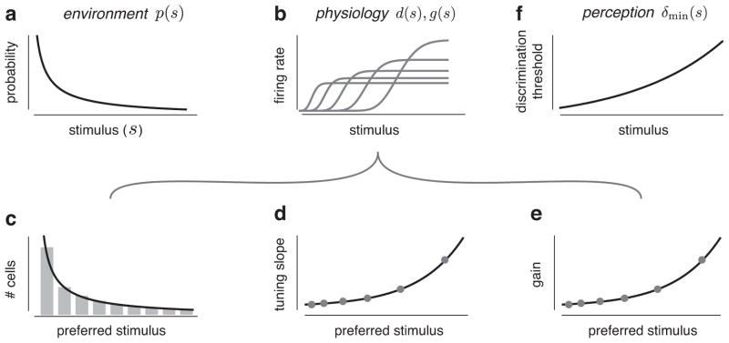
Figure 2.

Experimental predictions for efficient coding with a heterogeneous population of unimodal tuning curves. (a) Hypothetical example of a probability distribution over a sensory attribute, p(s). (b) Five tuning curves of a neural population arranged to maximize the amount of information transmitted about stimuli drawn from this distribution. (c–e) Predicted shapes of experimentally accessible attributes of the neural population, derived from the prior distribution using Eq. (14). (c) Histogram of the observed preferred stimuli (stimuli associated with the peaks of the tuning curves) provides an estimate of local cell density, d(s), which should be proportional to the prior distribution (black line). (d) Tuning widths of the neurons (measured as the full width at half maximum of the tuning curves) should be inversely proportional to the prior (points correspond to example neurons from (b)). (e) The gain, g(s), measured as the maximum average firing rate of each of the neurons, should be constant (points correspond to example neurons from (b)). (f) Minimum achievable discrimination thresholds of a perceptual system that relies on this efficient population are inversely proportional to the prior distribution (Eq. (16)).
2.5 Implications for perceptual discrimination
The optimal solution limits the best achievable discrimination performance of a perceptual system that bases its responses on the output of the population. Specifically, the Fisher information may be used to provide a lower bound on discriminability, even when the observer is biased (Seriès et al., 2009):
| (15) |
The constant Δ is determined by the threshold performance level in a discrimination task. Substituting the optimal solutions for d(s) and g(s) into Eq. (12), and substituting the resulting Fisher information into Eq. (15), gives the minimum achievable discrimination threshold:
| (16) |
This predicts that perceptual sensitivity (inverse discriminability) is proportional to the prior, such that more frequently occurring stimuli are easier to discriminate. The proportionality depends on the available resources {N, R}, the experimental conditions under which the thresholds were measured (Δ) and knowledge of the tuning curve shapes and tiling properties (Iconv). Even when these are not known, the shape of δmin(s) can be readily compared to experimental data (Fig. 2(f)). As a special case, note that variables with distributions that fall approximately as 1/s (a pseudo-prior, since it is not integrable) lead to discriminability δmin(s) ∝ s, which corresponds to the perceptual behavior commonly known as Weber’s law.
3 Inference and Decoding with Efficient Neural Populations
The structure of the efficient population has direct implications for Bayesian theories of perceptual inference, in which human observers are hypothesized to combine their noisy sensory measurements and prior knowledge of the environment to infer properties of the physical world (Knill and Richards, 1996; Simoncelli, 1993). A critical, but often overlooked issue in such models, is the means by which the brain obtains and represents prior knowledge (Simoncelli, 2009). The optimally efficient population developed in this article provides a potential substrate for answering this question, since the prior is implicitly represented in the arrangement of the tuning curves. In this section, we show that this implicit prior encoding provides a natural means of approximating posterior densities in a form that is readily integrated to compute expected values. Specifically, we derive a novel decoder – which we call the Bayesian population vector – that properly extracts and uses the implicit prior information to approximate the Bayes Least Squares estimate (i.e., the mean of the posterior). We demonstrate through simulations that the Bayesian population vector outperforms the standard population vector, converging to the true Bayesian estimator as N increases.
3.1 Posterior and Bayesian Population Vector
Probabilistic inference generally relies on the posterior distribution, p(s|r⃗), which may be written using Bayes’ rule as:
The likelihood, p(r⃗|s), is interpreted as a function of s evaluated for a single observation of r⃗, and the denominator is a normalizing constant.
In solving perceptual problems, the posterior is typically used in one of two ways. First, posterior distributions of a common variable that arise from independent measurements are combined multiplicatively (generally referred to as cue combination (Knill and Richards, 1996)). Products of likelihood functions are readily achieved with populations of neurons with Poisson spiking: the log likelihoods are linearly encoded in the spike counts of two neural populations, and the product of likelihoods is computed by pairwise addition of the spikes arising from corresponding neurons in the two populations (Ma et al., 2006). The optimal populations derived here can exploit the same computation to obtain a posterior distribution conditioned on both cues. Suppose the posterior of each cue individually is represented in a heterogeneous population, and that the tuning curves of the two populations are arranged identically to reflect the prior. The posterior conditioned on both cues (assuming the cues provide independent information) may be computed using a third heterogeneous population with the same tuning curve arrangement, that simply adds spikes from corresponding neurons in the two single-cue populations. The summed spikes represent the log of the product of likelihoods. But note that the priors of the two single-cue populations are not multiplied: the prior in the combined population is again encoded (implicitly) in the sampling of the tuning curves.
A second operation commonly performed on a posterior density is to integrate it, either for purposes of computing expected values, or of marginalization (partially integrating over some variables). The latter does not present any fundamental obstacle for the current framework, but is not relevant in the case of a one-dimensional (scalar) stimulus. For the former, we’ll first consider the particular case of the mean of the posterior, which corresponds to the Bayes least squares (BLS) estimator (also known as the minimum mean squared error estimator) of the variable s, given the noisy population response. The BLS estimate may be expressed as:
| (17) |
The continuous integrals in Eq. (17) can be approximated with discrete sums,
for any discrete set of stimulus values, sn, where δn is the spacing between adjacent values. The sums converge to their corresponding integrals in the limit as δn → 0. Assuming an efficient encoding population with sn the preferred stimuli of the tuning curves, the separation between curves is inversely proportional to the prior: .
Substituting this discretization into the expression above yields an approximation of the BLS estimator that correctly uses the prior information embedded in the population:
| (18) |
This approximation of the integral may be seen as a deterministic form of “importance sampling” (deterministic, because it uses the fixed values sn as the samples, rather than drawing them stochastically from the prior). Note that in this simple form, the prior is implicitly captured in the spacing/sampling of the tuning curves, and that the posterior expectation of any function f(·) can be approximated by replacing the sn in the numerator by f (sn). The use of non-uniform population sampling to embed priors for Bayesian decoding was first proposed in Shi and Griffiths (2009), and has been used to explain the relationship between the distribution of tuning preferences in neural populations and perceptual discrimination performance (Fischer and Peña, 2011; Girshick et al., 2011). More recently, it has been proposed as an explanation of perceptual biases that can arise in low signal-to-noise conditions (Wei and Stocker, 2012a).
It is worth noting that this discrete approximation exhibits a striking similarity to the population vector (PV) decoder (Georgopoulos et al., 1986), which computes a response-weighted average of the preferred stimuli of the cells:
| (19) |
By inspection, if one assumes rn ∝ p(r⃗|sn), then the population vector can be seen to approximate the BLS estimate (Fischer and Peña, 2011; Shi and Griffiths, 2009). However, this assumption is clearly violated by the Poisson response model of Eq. (1).
To derive a version of the BLS estimator that does not rely on this incorrect assumption, we expand the likelihood weights, p(r⃗|sn) according to Eq. (1), and substitute them into Eq. (18) to obtain:
| (20) |
In the second step, we use the tiling property of the efficient population, to cancel these common terms in the numerator and denominator. The term does not depend on n, and therefore also cancels in the numerator and denominator.
The term hm(sn) represents the mean response of the mth neuron to the stimulus preference of the nth neuron. Using Eq. (10), and the fact that the gain is constant for the optimal population, we see that hm(sn) ∝ h(D(sn) − m) = h(n − m). As a result, the term can be expressed as a convolution of the neural responses with a fixed discrete linear filter, wm = log h(m) (to avoid log of zero, we can assume h(m) includes an additive constant representing the spontaneous firing rate of the neurons). Incorporating this into Eq. (20), we obtain an expression for the discrete approximation to the Bayes least squares estimator, which we call the Bayesian population vector (BPV):
| (21) |
Note that this has the form of the standard population vector (Eq. (19), except that the responses are filtered and exponentiated. These operations convert the spike counts in r⃗, which are linearly related to the log likelihood (Jazayeri and Movshon, 2006; Ma et al., 2006), back into a form that is effectively proportional to the posterior probability.
The computation of the posterior density, and the expectation of any function over this posterior, can be implemented in a compact neural circuit (Fig. 3). Each downstream neuron linearly combines the spiking responses of neurons in the efficient population that have similar stimulus preferences, and the result is then exponentiated and normalized. These responses represent a sampled version of the posterior density. This set of operations – linear filtering, a rectifying nonlinearity, divisive normalization – have been implicated as canonical neural computations for hierarchical sensory processing (Carandini and Heeger, 2012; Kouh and Poggio, 2008). The expectation over the posterior distribution can then be computed as a sum of these responses, weighted by the function whose expectation is being computed:
| (22) |
Figure 3.

Computation of the posterior distribution, and the Bayesian population vector (BPV), from responses of an optimally efficient encoding population. (a) Hypothetical prior distribution over the stimulus variable. (b) Optimal encoding population. Colored tick marks denote the preferred stimuli, sn, of each neuron. Points represent (noisy) responses of each neuron to a particular stimulus value, with color indicating the preferred stimulus of the corresponding neuron. (c) The decoder convolves these responses with a linear filter (triplets of thin gray lines) with weights log h(m). The convolution output is exponentiated (boxes) and normalized by the sum over the decoder population, yielding an encoding of the posterior distribution, p(s|r⃗), whose integral against any function may then be approximated. As an example, the BPV is computed by summing these responses, weighted by their associated preferred stimulus values, to approximate the mean of the posterior, which is the Bayes least square estimate of the stimulus.
As an example, consider a signal classification problem, in which one must decide from which of two classes a stimulus was drawn by comparing probabilities p(c1|r⃗) and p(c2|r⃗). These two probabilities can each be written as an expectation over the posterior: p(ci|r⃗) = ∫ p(ci|s)p(s|r⃗) ds. As such, they can be approximated using the weighted sum in Eq. (22), with f(sn) = p(ci|sn). Note that the latter implicitly contain the class prior probabilities, since p(ci|sn) = p(sn|ci)p(ci)/p(sn).
3.2 Simulations
We find that the Bayesian population vector provides a good approximation to the true Bayes least squares estimator over a wide range of N and R values, and converges as either N or R increase. In contrast, we find that the standard population vector operating on the responses of an efficient population poorly approximates the BLS estimator for most values of N and R, and fails to converge. Furthermore, optimizing the weights of the standard population vector results in a significant improvement in performance, but the resulting estimator still fails to converge.
To compute the mean squared errors for the three estimators, we first drew 10, 000 samples from an exponential prior distribution with mean value 20, clipped to a maximum value of 60 (Fig. 3a). Next, we simulated the responses of neural populations, of size N with mean total spike rate R, designed to maximize information about stimuli drawn from this prior (Fig. 3b). The response of each neuron to a single stimulus value corresponds to a sample from a Poisson distribution, with the rate parameter determined by the neuron’s tuning curve evaluated at that stimulus value. From these neural responses, we computed stimulus estimates using the true Bayes least squares estimator (Eq. (17)) the Bayesian population vector (Eq. (21)), the standard population vector (Eq. (19)), and a standard population vector with stimulus values sn optimized to minimize the squared error of the estimates. We approximated the mean squared error of each of these estimators as the sample average of the square differences between the estimates and true stimulus values.
The mean squared error of the Bayesian population vector converges to that of the Bayes least squares estimator as the number of neurons increases, independent of the total mean firing rate (Fig. 4a). In a low firing rate regime (0.1 maximum average spikes/neuron) the approximation is within 1% of the true error with as few as 10 neurons. In this regime, the estimation error of the BLS estimator is significant, and the BPV is only slightly worse. Note, however, that for 10 neurons firing a maximum of 10 spikes each, the mean squared error of the BPV is 25% larger than that of the BLS estimator. In this regime, the likelihood is very narrow due to the abundance of spikes relative to the spacing of the preferred stimuli (which is inversely proportional to N). As a result, the discretized likelihood weights, p(r⃗|sn), become concentrated on the preferred stimulus value with the highest likelihood, and the BPV essentially behaves as a “winner-take-all” estimator, which is generally inferior to the true BLS estimator operating in the same resource regime.
Figure 4.

Relative estimation errors of three different decoders, computed on responses of an optimized heterogeneous population. All results are presented relative to the true Bayes least squares (BLS) decoder (e.g., a value of 1 indicates performance equal to the BLS). a The Bayesian population vector accurately approximates the true BLS estimator (in terms of mean squared error) over a wide range of resource constraints, and converges as the number of neurons increases. b The standard population vector has substantially larger error (note scale), and fails to converge to BLS performance levels. c Optimizing the weights of a population vector leads to a significant performance increase, but the resulting estimator is still substantially worse than the BPV and again fails to converge.
The population vector (PV) defined in Eq. (19) has been previously proposed as a means of computing approximate BLS estimates, but the approximation relies on strong assumptions about the encoding population (Fischer and Peña, 2011; Girshick et al., 2011; Shi and Griffiths, 2009; Wei and Stocker, 2012a). We find that the PV provides a reasonably accurate approximation to the BLS estimator in a low firing rate regime (0.1 maximum average spikes/neuron), but becomes increasingly suboptimal (by orders of magnitude) as the number of neurons increases (Fig. 4b). This is due to the fact that the population vector does not take likelihood width into account correctly, and is therefore biased by the asymmetries in the preferred stimuli (the implicitly encoded prior) even when the sensory evidence is strong.
The standard population vector can be improved by optimizing the weights, sn, in Eq. (19) so as to minimize the squared error. We simulated this optimal population vector (OPV), using weights optimized over the sampled data for each value of N. We find that this the OPV exhibits significant improvements in performance compared to the ordinary PV (Fig. 4c), but is still substantially worse than the BPV. And as with the PV, the OPV fails to converge to the true BLS estimator as N increases.
4 Extensions and generalizations
The efficient encoding framework developed in section 2 may be extended in a number of ways. Here, we explore the optimization of alternative objective functions, generalize our results to handle sigmoidal tuning curves, and examine the influence of non-Poisson firing rate models on our optimal solutions. We also discuss how these modifications to the encoding model affect the Bayesian decoding results developed in section 3.
4.1 Alternative objective functions
Although information maximization is a commonly assumed form of coding optimality for sensory systems, alternative objective functions have been proposed. Some authors have suggested that sensory representations might be directly optimized for minimizing estimation error (e.g., Brown and Bäcker, 2006; McDonnell and Stocks, 2008; Montemurro and Panzeri, 2006; Pouget et al., 1999; Zhang and Sejnowski, 1999) and others for minimizing perceptual discriminability (von der Twer and MacLeod, 2001; Wang et al., 2012). Our formulation, with a population parameterized by density and gain, is readily extended to these cases.
Consider a generalized objective function that aims to maximize the expected value of a function of the Fisher information:
| (23) |
The efficient coding case considered in the previous section corresponds to f(x) = log(x) – we refer to this as the infomax case. Choosing f(x) = − x−1 corresponds to maximizing the Fisher bound on squared discriminability (see Eqs. (12) & (15)) – we refer to this as the discrimax case. The more conventional interpretation of this objective function, is as a bound on the mean squared error of an unbiased estimator (Cox and Hinkley, 1974). However, the discriminability bound is independent of estimation bias and thus requires less assumptions about the form of the estimator. More generally, we can consider a power function, f(x) = xα, for some exponent α.
The solution for any exponent a is readily obtained using calculus of variations, and is given in Table 1. The infomax solution is included for comparison. In all cases, the solution specifies a power-law relationship between the prior, the density and gain of the tuning curves, and perceptual discrimination thresholds. In general, all solutions allocate more neurons, with correspondingly narrower tuning curves, resulting in smaller discrimination thresholds, for more probable stimuli. But the exponents vary, depending on the choice of α. The shape of the optimal gain function depends on the objective function: for α < 0, neurons with lower firing rates are used to represent stimuli with higher probabilities, and for α > 0, neurons with higher firing rates are used for stimuli with higher probabilities. As in the infomax case, the resource constraints, N and R, enter the solution as multiplicative scale factors, facilitating a comparison to data. As a result, the theory offers a framework within which existing data may be used to determine those optimality principles that best characterize different brain areas. It is worth noting that only the infomax solution leads to a neural encoding of prior information that can be extracted and used to produce Bayesian perceptual estimates using the logic developed in section 3 (see Discussion).
Table 1.
Closed form solution for optimal neural populations with unimodal tuning curves, for objective functions specified by Eq. (23).
| Infomax | Discrimax | General | ||||
|---|---|---|---|---|---|---|
|
| ||||||
| Optimized function: | f(x) = log x | f(x) = −x−1 |
|
|||
| Density (Tuning width)−1 | d(s) | Np(s) |
|
|
||
| Gain | g(s) | R |
|
|
||
| Fisher information | If (s) | ∝ RN2p2(s) |
|
|
||
| Discriminability bound | δmin(s) | ∝ p−1(s) |
|
|
||
4.2 Sigmoidal response functions
To derive the efficient population code in section 2, we assumed that the tuning curves “tile” the space (Eq. (7)). This assumption is incompatible with monotonically increasing sigmoidal response functions, as are observed for encoding intensity variables such as visual contrast or auditory sound pressure level. Nevertheless, we can use the continuous parameterization of cell density and gain to obtain an optimal solution for a population of neurons with sigmoidal responses.
To see this, we start by noting that the Fisher information of a homogeneous population of sigmoidal tuning curves is the same as in the unimodal case (Eq. (12)), again assuming that the Fisher information curves of the homogeneous population tile the space. The constraint on N is also unchanged from the unimodal case. However, the constraint on R is fundamentally different. For neurons with sigmoidal tuning curves, the entire population will be active for large stimulus values, which incurs a large metabolic cost for encoding these values. Intuitively, we might imagine that this metabolic penalty can be reduced by lowering the gains of neurons tuned to the low end of the stimulus range, or by adjusting the cell density such that there are more tuning curves selective for the high end of the stimulus range. But it is not obvious how the reductions in metabolic cost for these coding strategies should trade off with the optimal coding of sensory information.
To derive the optimal solution, we first parameterize a heterogeneous population of sigmoidal response curves by warping and scaling the derivatives of a homogeneous population:
| (24) |
Here, h(·) is a prototype sigmoidal response curve, and we assume that the derivative of this response curve is a unimodal function that tiles the stimulus space when sampled at unit spacing: . The warping function is again the cumulative integral of a cell density function, , so that d(·) controls both the density of tuning curves and their slopes.
The total spike count can be obtained by combining Eqs. (2) & (24):
We define a continuous version of the gain as , and integrate by parts to approximate the total number of spikes as:
where is the cumulative density function of the sensory prior. This constraint on the total number of spikes is very different than that of Eq. (13), and will thus affect the optimal solutions for cell density and gain.
The optimization problem now becomes
| (25) |
A closed-form optimum of this objective function may again be found by using calculus of variations and the method of Lagrange multipliers. Solutions are provided in Table 2 for the infomax, discrimax, and general power cases.
Table 2.
Closed form solution for optimal neural populations with sigmoidal tuning curves, for objective functions specified by Eq. (25).
| Infomax | Discrimax | General | |||||
|---|---|---|---|---|---|---|---|
|
| |||||||
| Optimized: | f(x) = log x | f(x) = −x−1 |
|
||||
| Density | d(s) | Np(s) |
|
|
|||
| Gain | g(s) | RN−1 [1 − P(s)]−1 | RN−1 [1 − P (s)]−1 | RN−1 [1 − P (s)]−1 | |||
| Fisher | If (s) | ∝ RNp2(s) [1 − P(s)]−1 |
|
|
|||
| Discrim. | δmin(s) |
|
|
|
|||
For all objective functions, the solutions for the optimal density, gain, and discriminability are products of power law functions of the sensory prior, and its cumulative distribution. In general, all solutions allocate more neurons with greater dynamic range to more frequently occurring stimuli. Note that, unlike the solutions for unimodal tuning curves (Table 1), the optimal gain is the same for all objective functions: for each neuron, the optimal gain is inversely proportional to the probability that a randomly chosen stimulus will be larger than its preferred stimulus. Intuitively, this solution allocates lower gains to neurons tuned to the low end of the stimulus range, which is metabolically less costly. The global resource values N and R again only appear as scale factors in the overall solution, allowing us to easily compare the predicted relationships to experimental data, even when N and R are not known (Fig. 5).
Figure 5.
Experimental predictions for efficient coding with sigmoidal tuning curves. Panels are analogous to Fig. 2, but illustrate the solution given in the infomax column of Table 2.
As in the unimodal case, the infomax solution yields a neural representation of prior information that can be easily extracted and used to produce Bayesian perceptual estimates. The estimator is similar in form to the BPV developed in section 3 with a single key difference: the sum of discretized tuning curves (middle terms in the numerator and denominator of Eq. (20)) is no longer a constant. Hence, this set of weights must be subtracted from the filtered neural responses, before the result is passed through the exponential.
4.3 Generalization to Poisson-like noise distributions
Our results depend on the assumption that the spike counts of neurons are Poisson-distributed and independent of each other. In a Poisson model, the variance of the spike counts is equal to their mean, which has been observed in some experimental situations (Britten et al., 1993; Tolhurst et al., 1983), but not all (e.g., Shadlen and Newsome, 1998; Werner and Mountcastle, 1963). In addition, the assumption that neuronal responses are statistically independent conditioned on the stimulus value is often violated (Kohn and Smith, 2005; Zohary et al., 1994).
Here, we show that our results can be generalized to a family of “Poisson-like” response models introduced by (Beck et al., 2007; Ma et al., 2006), that allow for stimulus dependent correlations and a more general linear relationship between the mean and variance of the population response:
| (26) |
This distribution belongs to the exponential family with linear sufficient statistics where the parameter η(s) is a vector of the natural parameters of the distribution with the nth element equal to ηn(s), a(η(s)) is a (log) normalizing constant that ensures the distribution integrates to one, and f(r⃗) is an arbitrary function of the firing rates. The independent Poisson noise model considered in Eq. (1) is a member of this family of distributions with parameters: η(s) = log h(s) where h(s) is a vector of tuning curve functions, with the nth element equal to hn(s), , and .
Our objective functions depend on an analytical form for the Fisher information in terms of tuning curves. The Fisher information for the response model in Eq. (26) may be expressed in terms of the Fisher information matrix of the natural parameters using the chain rule:
| (27) |
The Fisher information matrix about the natural parameters may be written as (Cox and Hinkley, 1974):
| (28) |
where Σ(s) = ER|S[r⃗ r⃗T] is the stimulus-conditioned covariance matrix of the population responses.
Finally, the derivative of the natural parameters may be written in terms of the derivatives of the tuning curves (Beck et al., 2007; Ma et al., 2006),
| (29) |
where Σ−1(s) is the inverse of the covariance matrix, also known as the precision matrix. Substituting Eqs. (29 & 28) into Eq. (27) yields the final expression for the local Fisher information:
| (30) |
The influence of Fisher information on coding accuracy is now directly dependent on knowledge of the precision matrix, which is difficult to estimate from experimental data (although see (Kohn and Smith, 2005)). Here, we assume a precision matrix that is consistent with neuronal variability that is proportional to the mean firing rate, as well as correlation of nearby neural responses (Abbott and Dayan, 1999). Specifically, for a homogeneous neural population, hn(s) = h(s − n), we express each element in the precision matrix as:
| (31) |
where δn,m is the Kronecker delta (zero, unless n = m, for which it is one). The parameter α controls a linear relationship between the mean response and the variance of the response for all the neurons. The parameter β controls the correlation between adjacent neurons. The Fisher information of a homogeneous population may now be expressed from Eqs. (30 & 31) as,
In the last step, we assume (as for the independent Poisson case) the Fisher information curves of the homogeneous population, ϕ(s − n) sum to a constant. We also assume that the cross terms, ψ(s − n, s − m), sum to the constant, Icorr.
The Fisher information for a heterogeneous population, obtained by warping and scaling the homogeneous population by the density and gain is
| (32) |
| (33) |
In the second step we make three assumptions. First, (as for the independent Poisson case) we assume g(s) is smooth relative to the width of ϕ(D(s) − n) for all n, so that we can approximate g(sn) as g(s). Second, we assume that the neurons are sufficiently dense such that . Finally, we assume g(s) is also smooth relative to the width of the cross terms, ψ(D(s) − n)ψ(D(s) − m). As a result, the gain factors can be approximated by the same continuous gain function, g(s), and can be pulled out of both sums.
The Fisher information expressed in Eq. (33) has the same dependency on s as that of the original Poisson population, but now depends on three parameters, α, β, and Icorr, that characterize the correlated variability of the population code. We conclude that the optimal solutions for the density and gain are the same as those expressed in Tables 1 & 2, which were derived for an independent Poisson noise model (α = 1, β = 0).
Because the solution for the infomax tuning curve density is the same as in the Poisson case (proportional to the prior), we can use the same logic developed in section 3 to derive a Bayes least squares estimator for the generalized response model that exploits the embedded prior. Specifically, we use the response model in Eq. (26) to expand out the likelihood weights in Eq. (18) to obtain:
In the second step, in addition to canceling out the terms f(r⃗) in the numerator and denominator, we again use the fact that the optimal population is obtained by warping a convolutional population. As a result, ηm(sn) corresponds to a set of weights that is the same for all m neurons. Therefore, the operation can be expressed as a convolution of the neural responses with a fixed linear filter w⃗. The filter weights will be different from those in the Poisson case, where the natural parameters are simply the log-tuning curves. The above expression is equivalent to the BPV for all response models where a(η(sn)) is constant for all sn. Otherwise, the above expression yields a BPV with an additional offset term, similar to the sigmoidal case.
5 Discussion
We have developed a formulation of the efficient coding hypothesis for a neural population encoding a scalar stimulus variable drawn from a known prior distribution. The information-maximizing solution provides precise and yet intuitive predictions of the relationship between sensory priors, physiology, and perception. Specifically, more frequently occurring stimuli should be encoded with a proportionally higher number of cells (with correspondingly narrower tuning widths) which results in a proportionally higher perceptual sensitivity for these stimulus values. Preliminary evidence indicates that these predictions are consistent with environmental, physiological, and perceptual data collected for a variety of visual and auditory sensory attributes (Ganguli, 2012; Ganguli and Simoncelli, 2010). We have also shown that the efficient population encodes prior information in a form that may be naturally incorporated into subsequent processing. Specifically, we have defined a neurally-plausible computation of the posterior distribution from the population responses, thus providing a hypothetical framework by which the brain might implement probabilistic inference. Finally, we developed extensions of the framework to consider alternative objective functions, sigmoidal response functions, and non-Poisson response noise.
Our framework naturally generalizes previous results on optimal coding with single neurons (Fairhall et al., 2001; Laughlin, 1981; McDonnell and Stocks, 2008; von der Twer and MacLeod, 2001; Wang et al., 2012), homogeneous population codes (Brown and Bäcker, 2006; Montemurro and Panzeri, 2006; Pouget et al., 1999; Zhang and Sejnowski, 1999), and heterogeneous populations with identical tuning curve widths (Brunel and Nadal, 1998; Harper and McAlpine, 2004), by explicitly taking into account heterogeneities in the environment and the tuning properties of sensory neurons, and by considering a family of optimality principles. Furthermore, our results are complementary to recent theories of how the brain performs probabilistic computations (Jazayeri and Movshon, 2006; Ma et al., 2006), providing an alternative framework for the encoding and use of prior information that extends and refines several recent proposals (Fischer and Peña, 2011; Ganguli and Simoncelli, 2012; Girshick et al., 2011; Shi and Griffiths, 2009; Simoncelli, 2009; Wei and Stocker, 2012a).
Our analysis requires several approximations and assumptions in order to arrive at an analytical solution for the optimal encoding population. First, we rely on lower bounds on mutual information and discriminability, each based on Fisher information. Note that we do not require the bounds on either information or discriminability to be tight, but rather that their optima be close to those of their corresponding true objective functions. It is known that Fisher information can provide a poor bound on mutual information for small numbers of neurons, low spike counts (or short decoding times), or non-smooth tuning curves (Bethge et al., 2002; Brunel and Nadal, 1998). It is also known that it can provide a poor bound on supra-threshold discriminability (Berens et al., 2009; Shamir and Sompolinsky, 2006). Nevertheless, we have found that, at least for typical experimental settings and physiological data sets, the Fisher information provides a reasonably tight bound on mutual information (Ganguli, 2012).
We made several assumptions in parameterizing the heterogeneous population: (1) the tuning curves, h(D(s) − n) (or in the sigmoidal case, their derivatives) evenly tile the stimulus space; (2) the single neuron Fisher information kernels, ϕ(D(s) − n), evenly tile the stimulus space; and (3) the gain function, g(s), varies slowly and smoothly over the width of h(D(s) − n) and ϕ(D(s) − n). These assumptions allow us to approximate Fisher information in terms of cell density and gain (Fig. 1(e)), to express the resource constraints in simple form, and to obtain a closed-form solution to the optimization problem.
Our framework is limited by the primary simplification used throughout the population coding literature: the tuning curve response model is restricted to a single (one-dimensional) stimulus attribute. Real sensory neurons exhibit selectivity for multiple attributes. If the prior distribution for those attributes is separable (i.e., if the values of those attributes are statistically independent) then an efficient code can be constructed separably. That is, each neuron could have joint tuning arising from the product of a tuning curve for each attribute. Extending the theory to handle multiple attributes with statistical dependencies is not straightforward, and seems likely to require additional constraints to obtain a unique solution, since there are many ways of carving a multi-dimensional input distribution into equal-size portions of probability mass. Furthermore, physiological and perceptual experiments are commonly restricted to only measure responses to one-dimensional stimulus attributes. As such, a richer theory that incorporates a multi-dimensional encoding model will not be easily tested with existing data.
The Bayesian population vector offers an example of how the optimal population may be properly incorporated into inferential computations that can be used to describe perception and action. The defining characteristic of this solution is the implicit embedding of the prior in the distribution and shapes of tuning curves within the encoding population, eliminating the need for a separate “prior-encoding” neural population (Ma et al., 2006; Yang et al., 2012), and generalizing previous proposals for representing priors solely with neural gains (Simoncelli, 2003), the sum of tuning curves (Simoncelli, 2009), or the distribution of tuning preferences (Fischer and Peña, 2011; Girshick et al., 2011; Shi and Griffiths, 2009). Furthermore, if one assumes tuning curves that include a baseline response level (i.e., a background firing rate), the efficient population will also exhibit spontaneous responses reflecting the environmental prevalence of stimuli, which is consistent with recent predictions that that spontaneous population activity provides an observable signature of embedded prior probabilities (Berkes et al., 2011; Tkačik et al., 2010).
Nevertheless, it seems unlikely that the brain would implement a decoder that explicitly transforms the distributed population activity into a single response value. A more likely scenario arises from retaining the population representation of the posterior (Fig. 3, with the final summation omitted) and performing subsequent computations such as multiplication by other sensory posteriors (Ma et al., 2006), or marginalization (Beck et al., 2011) only when necessary for action (Simoncelli, 2009). One final caveat is that the decoder considered here (both the posterior computation, as well as the full BPV) is deterministic, and a realistic solution for neural inference will need to incorporate the effects of neural noise introduced at each stage of processing (Sahani and Dayan, 2003; Stocker and Simoncelli, 2006).
At a more abstract level, the efficient population solution has two counterintuitive implications regarding the implementation of Bayesian inference in a biological system. First, we note that of the family of encoding solutions derived in Tables 1 & 2, only the infomax solution leads to a neural encoding of prior information that can be extracted and used to produce Bayesian perceptual estimates using the logic developed in section 3. The discrimax solution, which is optimized for minimizing squared error (assuming an unbiased estimator) does not lend itself to an encoding of prior information that is amenable to a simple implementation of Bayesian decoding. Despite the inconsistency of the infomax and MSE objective functions, we find it intuitively appealing that early-stage sensory encoding should be optimized bottom-up for a general (task-free) objective like information transmission, while later-stage decoding is more likely optimized for solving particular problems, such as least-squares estimation or comparison of stimulus attributes. Second, Bayesian estimators are traditionally derived from pre-specified likelihood, prior, and loss functions, each of which parameterize distinct and unrelated aspects of the estimation problem: the measurement noise, the environment, and the estimation task or goal. But in the efficient population, the likelihood is adaptively determined by the prior, and thus, the estimator is entirely determined by the loss function and the prior. As a result, in addition to the predictions of physiological attributes and perceptual discriminability that we derived from our encoding framework, it should also be possible to predict the form of perceptual biases (see (Wei and Stocker, 2012b) for an example).
Finally, if the efficient population we’ve described is implemented in the brain, it must be learned from experience. It seems implausible that this would be achieved by direct optimization of information, as was done in our derivation. Rather, a simple set of rules could provide a sufficient proxy to achieve the same solution (e.g., Doi et al., 2012). For example, if each neuron in a population adjusted its tuning curve so as to (1) achieve response distributions with mean and variance values that are the same across the population; (2) ensure that the input domain is “tiled” (leaving no gaps); and 3) allow only modest levels of redundancy with respect to responses of other cells in the population, then we conjecture that the resulting population would mimic the efficient coding solution. Moreover, allowing the first adjustment to occur on a more rapid timescale than the others could potentially account for widely observed adaptation effects, in which the gain of individual neurons is adjusted so as to maintain a roughly constant level of activity (Benucci et al., 2013; Fairhall et al., 2001). If such adaptive behaviors could be derived from our efficient coding framework, and reconciled with the underlying circuitry and cellular biophysics, the resulting framework would provide a canonical explanation for the remarkable ability of sensory systems to adapt to and exploit the statistical properties of the environment.
Acknowledgments
We thank Wei Ji Ma and the reviewers for helpful discussions and suggestions.
Contributor Information
Deep Ganguli, Email: dganguli@cns.nyu.edu.
Eero P. Simoncelli, Email: eero.simoncelli@nyu.edu.
References
- Abbott L, Dayan P. The effect of correlated variability on the accuracy of a population code. Neural Computation. 1999;11(1):91–101. doi: 10.1162/089976699300016827. [DOI] [PubMed] [Google Scholar]
- Atick J, Redlich A. Towards a theory of early visual processing. Neural Computation. 1990;2(3):308–320. [Google Scholar]
- Attneave F. Some informational aspects of visual perception. Psychological Review. 1954;61(3):183–193. doi: 10.1037/h0054663. [DOI] [PubMed] [Google Scholar]
- Barlow H. Possible principles underlying the transformation of sensory messages. Sensory Communication. 1961:217–234. [Google Scholar]
- Beck J, Latham P, Pouget A. Marginalization in neural circuits with divisive normalization. The Journal of Neuroscience. 2011;31(43):15310–15319. doi: 10.1523/JNEUROSCI.1706-11.2011. [DOI] [PMC free article] [PubMed] [Google Scholar]
- Beck J, Ma W, Latham P, Pouget A. Probabilistic population codes and the exponential family of distributions. Prog Brain Res. 2007;165:509–519. doi: 10.1016/S0079-6123(06)65032-2. [DOI] [PubMed] [Google Scholar]
- Bell A, Sejnowski T. The ”independent components” of natural scenes are edge filters. Vision Research. 1997;37(23):3327–3338. doi: 10.1016/s0042-6989(97)00121-1. [DOI] [PMC free article] [PubMed] [Google Scholar]
- Benucci A, Saleem AB, Carandini M. Adaptation maintains population homeostasis in primary visual cortex. Nature Neuroscience. 2013;16(6):724–729. doi: 10.1038/nn.3382. [DOI] [PMC free article] [PubMed] [Google Scholar]
- Berens P, Gerwinn S, Ecker A, Bethge M. Neurometric function analysis of population codes. Advances in Neural Information Processing Systems. 2009;22:90–98. [Google Scholar]
- Berkes P, Orbán G, Lengyel M, Fiser J. Spontaneous cortical activity reveals hallmarks of an optimal internal model of the environment. Science. 2011;331(6013):83–87. doi: 10.1126/science.1195870. [DOI] [PMC free article] [PubMed] [Google Scholar]
- Bethge M, Rotermund D, Pawelzik K. Optimal short-term population coding: When fisher information fails. Neural Computation. 2002;14(10):2317–2351. doi: 10.1162/08997660260293247. [DOI] [PubMed] [Google Scholar]
- Britten K, Shadlen M, Newsome W, Movshon J. Responses of neurons in macaque MT to stochastic motion signals. Visual neuroscience. 1993;10(6):1157–1169. doi: 10.1017/s0952523800010269. [DOI] [PubMed] [Google Scholar]
- Brown W, Bäcker A. Optimal neuronal tuning for finite stimulus spaces. Neural Computation. 2006;18(7):1511–1526. doi: 10.1162/neco.2006.18.7.1511. [DOI] [PubMed] [Google Scholar]
- Brunel N, Nadal J. Mutual information, fisher information, and population coding. Neural Computation. 1998;10(7):1731–1757. doi: 10.1162/089976698300017115. [DOI] [PubMed] [Google Scholar]
- Carandini M, Heeger D. Normalization as a canonical neural computation. Nature Reviews Neuroscience. 2012;13(1):51–62. doi: 10.1038/nrn3136. [DOI] [PMC free article] [PubMed] [Google Scholar]
- Cover T, Thomas J. Elements of information theory. Wiley-Interscience. Published; Hardcover: 1991. [Google Scholar]
- Cox D, Hinkley D. Theoretical statistics. London: Chapman and Hall; 1974. [Google Scholar]
- Doi E, Gauthier J, Field G, Shlens J, Sher A, Greschner M, Machado T, Jepson L, Mathieson K, Gunning D, Litke A, Paninski L, Chichilnisky EJ, Simoncelli EP. Efficient coding of spatial information in the primate retina. J Neuroscience. 2012 doi: 10.1523/JNEUROSCI.4036-12.2012. To appear. [DOI] [PMC free article] [PubMed] [Google Scholar]
- Fairhall A, Lewen G, Bialek W, de Ruyter van Steveninck R. Efficiency and ambiguity in an adaptive neural code. Nature. 2001;412(6849):787–792. doi: 10.1038/35090500. [DOI] [PubMed] [Google Scholar]
- Fischer B, Peña J. Owl’s behavior and neural representation predicted by bayesian inference. Nature Neuroscience. 2011;14(8):1061–1066. doi: 10.1038/nn.2872. [DOI] [PMC free article] [PubMed] [Google Scholar]
- Ganguli D. PhD thesis. Center for Neural Science, New York University; New York, NY: 2012. Efficient coding and Bayesian inference with neural populations. [Google Scholar]
- Ganguli D, Simoncelli E. Implicit encoding of prior probabilities in optimal neural populations. In: Lafferty J, Williams C, Shawe-Taylor J, Zemel R, Culotta A, editors. Advances in Neural Information Processing Systems (NIPS) Vol. 23. Salt Lake City, Utah: 2010. pp. 658–666. [PMC free article] [PubMed] [Google Scholar]
- Ganguli D, Simoncelli E. Computational and Systems Neuroscience (CoSyNe) Salt Lake City, Utah: 2012. Neural implementation of bayesian inference using efficient population codes. [Google Scholar]
- Geisler W, Najemnik J, Ing A. Optimal stimulus encoders for natural tasks. Journal of Vision. 2009;9(13):17, 1–16. doi: 10.1167/9.13.17. [DOI] [PMC free article] [PubMed] [Google Scholar]
- Georgopoulos A, Schwartz A, Kettner R. Neuronal population coding of movement direction. Science. 1986;233(4771):1416–1419. doi: 10.1126/science.3749885. [DOI] [PubMed] [Google Scholar]
- Gersho A, Gray R. Vector quantization and signal compression. Kluwer Academic Publishers; Norwell, MA: 1991. [Google Scholar]
- Girshick A, Landy M, Simoncelli E. Cardinal rules: visual orientation perception reflects knowledge of environmental statistics. Nature Neuroscience. 2011;14(7):926–932. doi: 10.1038/nn.2831. [DOI] [PMC free article] [PubMed] [Google Scholar]
- Harper N, McAlpine D. Optimal neural population coding of an auditory spatial cue. Nature. 2004;430(7000):682–686. doi: 10.1038/nature02768. [DOI] [PubMed] [Google Scholar]
- Helmholtz H. Treatise on physiological optics. Thoemmes Press; Bristol, UK: 2000. [Google Scholar]
- Jazayeri M, Movshon J. Optimal representation of sensory information by neural populations. Nature Neuroscience. 2006;9(5):690–696. doi: 10.1038/nn1691. [DOI] [PubMed] [Google Scholar]
- Karklin Y, Simoncelli E. Efficient coding of natural images with a population of noisy linear-nonlinear neurons. Adv Neural Information Processing Systems (NIPS*11); Presented at Neural Information Processing Systems 24; Granada, Spain. Dec 13–15 2011; Cambridge, MA: MIT Press; 2012. [PMC free article] [PubMed] [Google Scholar]
- Knill D, Richards W. Perception as Bayesian inference. Cambridge University Press; Cambridge, UK: 1996. [Google Scholar]
- Kohn A, Smith M. Stimulus dependence of neuronal correlation in primary visual cortex of the macaque. The Journal of Neuroscience. 2005;25(14):3661–3673. doi: 10.1523/JNEUROSCI.5106-04.2005. [DOI] [PMC free article] [PubMed] [Google Scholar]
- Kouh M, Poggio T. A canonical neural circuit for cortical nonlinear operations. Neural Computation. 2008;20(6):1427–1451. doi: 10.1162/neco.2008.02-07-466. [DOI] [PubMed] [Google Scholar]
- Laughlin S. A simple coding procedure enhances a neuron’s information capacity. Zeitschrift Für Naturforschung. 1981;36(9–10):910–912. [PubMed] [Google Scholar]
- Ma W, Beck J, Latham P, Pouget A. Bayesian inference with probabilistic population codes. Nature Neuroscience. 2006;9(11):1432–1438. doi: 10.1038/nn1790. [DOI] [PubMed] [Google Scholar]
- McDonnell M, Stocks N. Maximally informative stimuli and tuning curves for sigmoidal rate-coding neurons and populations. Physical Review Letters. 2008;101(5):58103. doi: 10.1103/PhysRevLett.101.058103. [DOI] [PubMed] [Google Scholar]
- Montemurro M, Panzeri S. Optimal tuning widths in population coding of periodic variables. Neural Computation. 2006;18(7):1555–1576. doi: 10.1162/neco.2006.18.7.1555. [DOI] [PubMed] [Google Scholar]
- Nadal J, Parga N. Non linear neurons in the low noise limit: A factorial code maximizes information transfer. Network: Computation in Neural Systems 1994
- Pouget A, Dayan P, Zemel R. Inference and computation with population codes. Annu Rev Neurosci. 2003;26:381–410. doi: 10.1146/annurev.neuro.26.041002.131112. [DOI] [PubMed] [Google Scholar]
- Pouget A, Deneve S, Ducom J, Latham P. Narrow versus wide tuning curves: What’s best for a population code? Neural Computation. 1999;11(1):85–90. doi: 10.1162/089976699300016818. [DOI] [PubMed] [Google Scholar]
- Sahani M, Dayan P. Doubly distributional population codes: Simultaneous representation of uncertainty and multiplicity. Neural Computation. 2003;15(10):2255–2279. doi: 10.1162/089976603322362356. [DOI] [PubMed] [Google Scholar]
- Salinas E, Abbott L. Vector reconstruction from firing rates. Journal of Computational Neuroscience. 1994;1(1–2):89–107. doi: 10.1007/BF00962720. [DOI] [PubMed] [Google Scholar]
- Sanger T. Probability density estimation for the interpretation of neural population codes. J Neurophysiol. 1996;76(4):2790–2793. doi: 10.1152/jn.1996.76.4.2790. [DOI] [PubMed] [Google Scholar]
- Seriès P, Stocker A, EPS Is the homunculus “aware” of sensory adaptation? Neural Computation. 2009;21(12):3271–3304. doi: 10.1162/neco.2009.09-08-869. [DOI] [PMC free article] [PubMed] [Google Scholar]
- Seung H, Sompolinsky H. Simple models for reading neuronal population codes. Proc National Academy of Sciences. 1993;90(22):10749–10753. doi: 10.1073/pnas.90.22.10749. [DOI] [PMC free article] [PubMed] [Google Scholar]
- Shadlen MN, Newsome WT. The variable discharge of cortical neurons: Implications for connectivity, computation, and information coding. The Journal of Neuroscience. 1998;18(10):3870–3896. doi: 10.1523/JNEUROSCI.18-10-03870.1998. [DOI] [PMC free article] [PubMed] [Google Scholar]
- Shamir M, Sompolinsky H. Implications of neuronal diversity on population coding. Neural Computation. 2006;18(8):1951–1986. doi: 10.1162/neco.2006.18.8.1951. [DOI] [PubMed] [Google Scholar]
- Shi L, Griffiths T. Neural implementation of hierarchical bayesian inference by importance sampling. NIPS. 2009:1669–1677. [Google Scholar]
- Simoncelli E. PhD thesis. Department of Electrical Engineering and Computer Science, Massachusetts Institute of Technology; Cambridge, MA: 1993. Distributed Analysis and Representation of Visual Motion. Also available as MIT Media Laboratory Vision and Modeling Technical Report #209. [Google Scholar]
- Simoncelli E. Optimal estimation in sensory systems. In: Gazzaniga M, editor. The Cognitive Neurosciences, IV. MIT Press; 2009. pp. 525–535. [Google Scholar]
- Simoncelli E, Olshausen B. Natural image statistics and neural representation. Annual Review of Neuroscience. 2001;24(1):1193–1216. doi: 10.1146/annurev.neuro.24.1.1193. [DOI] [PubMed] [Google Scholar]
- Simoncelli EP. Local analysis of visual motion. In: Chalupa LM, Werner JS, editors. The Visual Neurosciences. Vol. 109. MIT Press; 2003. pp. 1616–1623. [Google Scholar]
- Snippe H. Parameter extraction from population codes: A critical assessment. Neural Computation. 1996;8(3):511–529. doi: 10.1162/neco.1996.8.3.511. [DOI] [PubMed] [Google Scholar]
- Stocker A, Simoncelli E. Noise characteristics and prior expectations in human visual speed perception. Nature Neuroscience. 2006;9(4):578–585. doi: 10.1038/nn1669. [DOI] [PubMed] [Google Scholar]
- Tkačik G, Prentice JS, Balasubramanian V, Schneidman E. Optimal population coding by noisy spiking neurons. Proc National Academy of Sciences. 2010;107(32):14419–14424. doi: 10.1073/pnas.1004906107. [DOI] [PMC free article] [PubMed] [Google Scholar]
- Tolhurst D, Movshon J, Dean A. The statistical reliability of signals in single neurons in cat and monkey visual cortex. Vision Research. 1983;23(8):775–785. doi: 10.1016/0042-6989(83)90200-6. [DOI] [PubMed] [Google Scholar]
- von der Twer T, MacLeod D. Optimal nonlinear codes for the perception of natural colours. Network. 2001;12(3):395–407. [PubMed] [Google Scholar]
- Wang Z, Stocker A, Lee D. Optimal neural tuning curves for arbitrary stimulus distributions: Discrimax, infomax and minimum lp loss. Advances in Neural Information Processing Systems. 2012;25 [Google Scholar]
- Wei X, Stocker A. Bayesian inference with efficient neural population codes. Int’l Conf on Artificial Neural Networks (ICANN); Lausanne, Switzerland. 2012a. [Google Scholar]
- Wei X, Stocker A. Efficient coding provides a direct link between prior and likelihood in perceptual bayesian inference. Advances in Neural Information Processing Systems. 2012b;25:1313–1321. [Google Scholar]
- Werner G, Mountcastle VB. The variability of central neural activity in a sensory system, and its implications for the central reflection of sensory events. Journal of Neurophysiology. 1963;26(6):958–977. doi: 10.1152/jn.1963.26.6.958. [DOI] [PubMed] [Google Scholar]
- Yang J, Lee J, Lisberger S. The interaction of Bayesian priors and sensory data and its neural circuit implementation in visually-guided movement. J Neurosci. 2012;32:17632–17645. doi: 10.1523/JNEUROSCI.1163-12.2012. [DOI] [PMC free article] [PubMed] [Google Scholar]
- Zemel R, Dayan P, Pouget A. Probabilistic interpretation of population codes. Neural Computation. 1998;10(2):403–430. doi: 10.1162/089976698300017818. [DOI] [PubMed] [Google Scholar]
- Zhang K, Ginzburg I, McNaughton B, Sejnowski T. Interpreting neuronal population activity by reconstruction: Unified framework with application to hippocampal place cells. Journal of Neurophysiology. 1998;79(2):1017–1044. doi: 10.1152/jn.1998.79.2.1017. [DOI] [PubMed] [Google Scholar]
- Zhang K, Sejnowski T. Neuronal tuning: To sharpen or broaden? Neural Computation. 1999;11(1):75–84. doi: 10.1162/089976699300016809. [DOI] [PubMed] [Google Scholar]
- Zohary E, Shadlen M, Newsome W. Correlated neuronal discharge rate and its implications for psychophysical performance. Nature. 1994;370(6485):140–143. doi: 10.1038/370140a0. [DOI] [PubMed] [Google Scholar]