A control systems engineering approach for adaptive behavioral interventions: illustration with a fibromyalgia intervention

Abstract

The term adaptive intervention has been used in behavioral medicine to describe operationalized and individually tailored strategies for prevention and treatment of chronic, relapsing disorders. Control systems engineering offers an attractive means for designing and implementing adaptive behavioral interventions that feature intensive measurement and frequent decision-making over time. This is illustrated in this paper for the case of a low-dose naltrexone treatment intervention for fibromyalgia. System identification methods from engineering are used to estimate dynamical models from daily diary reports completed by participants. These dynamical models then form part of a model predictive control algorithm which systematically decides on treatment dosages based on measurements obtained under real-life conditions involving noise, disturbances, and uncertainty. The effectiveness and implications of this approach for behavioral interventions (in general) and pain treatment (in particular) are demonstrated using informative simulations.

INTRODUCTION

Advances in understanding disease and developing efficacious treatments, coupled with the challenge of rising health-care costs, have resulted in an increased interest within the field of behavioral medicine for developing more effective strategies to treat chronic, relapsing disorders [1, 2]. Conventional clinical practice is traditionally based on treatment plans designed for a standard response that may not recognize individual participant characteristics or apply optimization procedures. During a typical treatment phase, clinicians assess the response of a participant to treatment by noting changes in symptoms or expected outcomes and suggesting changes in treatment dosages (if required). Many of these treatment strategies are inspired from the acute care model and, in spite of efficacious treatments, are not necessarily well suited for chronic disorders. Hence, even with clinical histories available, the process of assigning treatment dosages by clinicians is based more or less on intuition and experience and may be not individualized.

One promising approach lies in adaptive behavioral interventions; these adjust treatment dosages over the course of the intervention based on the values of tailoring variables, that is, measures of participant response or adherence [3]. In this paper, we describe how control systems engineering [4] offers a novel and potentially powerful framework for optimizing the effectiveness of broad classes of adaptive behavioral interventions. Specifically, the development of decision policies from control engineering coupled with technological enhancements in information and computer technology can result in adaptive interventions that minimize waste, increase compliance, and enhance overall intervention potency [5–9]. By relying on repeated assessments of participant response and model-based operationalized treatment decisions, it is possible to ascertain the optimal treatment regimen for an individual participant with less active involvement of a clinician, ultimately improving intervention outcomes while lowering costs.

Consider an illustration from a hypothetical smoking cessation intervention. The participant is given a smartphone to track her daily craving and smoking, while taking a certain recommended fixed treatment, such as a nominal dose of bupropion or behavioral therapy scheduled at regular intervals. This mode of operation can be termed as “open-loop” because the treatment dosages are not adjusted based on participant response and may be suboptimal. Subsequently, the intervention can be switched to a “closed-loop” system where a “controller” (or decision algorithm) alters dosages over time based on the information provided by the participant. The smartphone records symptom severity and automatically suggests proper dosage changes based on a model of participant’s response to treatment, other assessment information, and clinical constraints. Data can still be sent periodically to clinicians for review, and flags can be set to trigger alerts to the clinician in case of an unexpected response. In this way, the best dosage levels can be determined with minimal time required on the part of clinicians and participants. The computer (or smartphone) can then continue to monitor symptoms (perhaps changing sampling frequency to once a week or once month) and make changes periodically as the individual’s response to treatment changes over time. It is important to note that in the closed-loop, the decisions are made by incorporating dynamics of the behavioral process, optimization on the basis of an objective function criterion, and clinical constraints as discussed in the rest of the paper.

We illustrate how control engineering can accomplish this vision for behavioral interventions with the treatment of fibromyalgia (FM), a complex, multi-symptom illness [10–12]. The approach is based on a secondary analysis of intensive longitudinal data collected in a previously conducted clinical trial that relied on low-dose naltrexone for the treatment of FM. We apply a data-based modeling technique from engineering known as system identification [13] to develop dynamical system models which model symptom changes over time from daily diary reports completed by intervention participants. We apply an idiographic approach [14, 15] and use these diary reports which include self-assessments of outcomes of interest (e.g., general pain symptoms, sleep quality) and additional external variables that affect these outcomes (e.g., stress, anxiety, and mood). The various psychosocial variables measured in the intervention, along with the pharmaceutical arm, are used to explain changes in reported pain and other symptoms. The estimated dynamical systems models then serve as the basis for applying a control technology known as model predictive control (MPC) as a decision algorithm for automatic dosage selection of naltrexone. A multiple degree-of-freedom formulation for MPC is presented that enables a clinician to adjust the speed at which a desired target pain level should be reached, with the capability to adjust to both anticipated and unanticipated changes in symptoms (as well as possible side effects) independently in the closed-loop system. Simulation results are presented to illustrate the performance of the proposed decision scheme that incorporates individual participant response, clinical constraints, modeling errors, and variability typically present in a real-life application.

While the treatment of FM with naltrexone serves as the primary example in this paper, similar procedures can be applied to many other disease-treatment combinations associated with behavioral medicine. Published work that examines aspects of the control systems engineering approach described in this paper in other behavioral health settings includes work on prevention of conduct disorder [8, 16–18], promotion of moderate-to-vigorous physical activity [19], general weight change and body composition [20], gestational weight gain [21–24], and smoking cessation [25–28].

The paper is organized as follows: the second section describes an approach for dynamical systems modeling with an example from the secondary analysis performed on the naltrexone intervention data. The third section demonstrates the application of a closed-loop control for assigning treatment adaptively using simulations based on the models estimated in the second section. The paper ends with a summary and conclusions in the fourth section that includes a brief discussion on the design of experimental protocols for behavioral interventions from a system identification perspective, motivated by the results of this study.

A DYNAMICAL SYSTEMS APPROACH FOR MODELING BEHAVIORAL INTERVENTIONS

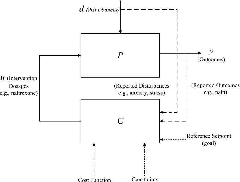
Dynamical systems modeling considers how to characterize the transient response resulting from changes in manipulated inputs (e.g., intervention components, denoted by u) and disturbance inputs (e.g., external influences which are not manipulated by the user, denoted by d) on outputs (e.g., proximal or distal outcomes, mediators, denoted by y) measured in an intensive longitudinal setting. In a typical pain intervention, the input (u) can represent the dosage of a primary intervention component like medication or counseling, while a disturbance (d) can correspond to behavioral constructs associated with the disorder that influence the outcomes but are independent of treatment, for example, a reported level of anxiety or stress. The output (y) can be an outcome of interest which the intervention aims to modify such as reported pain or sleep quality. In Fig. 1, we show that these three variables can be related to each other by the model P which is a symbolic representation of a dynamical system. P can be mathematically expressed using a system of ordinary differential equations (in continuous time t) or a system of difference equations (in sampled or discrete time k) among various other representations. A dynamical systems approach allows for an efficient mapping of the causal relationship between variables by capturing the concepts of change and effect in interventions. A representative dynamical system that incorporates many of the responses seen in this study is

1

Fig 1.

An input–output “block” diagram representation of the effect of input dosage (u) and disturbance (d) on output (y) using a dynamical system (P) in an open-loop configuration. The input u (e.g., dosages) induces, based on the system dynamics P, a resulting output y (e.g., pain report) in the presence of external disturbances d (e.g., symptoms such as anxiety and stress)

Since treatment dosages can change over time, they are represented as function of time or u(t). Equation (1) relates changes in the output y(t) and its derivatives with the changes in the input u(t) and its derivatives; K_p represents the process gain of the system which corresponds to the overall steady-state effect following a unit “step” change in the input. The parameters τ (natural time constant) and ζ (damping ratio) are related to the speed and shape of the time-domain response. For example, if ζ is less than 1, this would result in a decaying oscillatory response. The parameter τ_a (called the system zero) determines the initial direction of the symptom report in response to a dosage change.

In Fig. 2, we show a hypothetical case where a unit step change in the input u(t) is prescribed. The change in an outcome of interest y(t) (for example, the pain report provided by a participant) resulting from this input change can be observed. Different values of the coefficients in the differential equation (as shown in the legend of Fig. 2) result in responses of varying speed and shape; these range from a decaying-oscillatory response over time to a more sluggish, nonoscillatory response. Figure 2 also depicts an “inverse response” where τ_a is a negative number, which causes the response to initially increase prior to decreasing to a final steady-state value (solid blue line in Fig. 2). This transient response can be further quantified using dynamical system properties such as the rise time T_r (which is the time at which the response reaches 90 % of the steady state for the first time [29]) and the settling time T_s (which is the time when the response reaches 98 % of its steady-state value [29]). Brevity prevents a more detailed discussion, but we note that the second-order system structure shown in Eq. (1) can represent a highly diverse range of dynamical system responses observed in real life, among these mechanical, electrical, and process systems applications [29, 30].

Fig 2.

Representative time-domain responses of an output following a “step” change in the input for a second-order system according to Eq. (1). In this case, a unit change in treatment dosage at time t = 0 results in a 20 magnitude decrease in a symptom report over time. Based on the system dynamics, the responses range from a decaying oscillation with inverse response (solid blue line) to increasing sluggish, nonoscillatory response (red (dash), green (dot), and maroon (dash-dot))

The model structure shown in Eq. (1) can be extended to behavioral settings and, in the experience of the authors, representative of a large class of dynamical system responses in behavioral medicine. This will be shown in the paper with respect to fibromyalgia, but models within the general class of second-order systems have been observed in the modeling of smoking cessation [25], human weight and body composition change [20], and physical activity [19]. Statistically sound, data-centric procedures will be presented to estimate and validate these models; the procedures will similarly indicate when it is necessary to use higher order structures.

The data

FM is a disorder characterized primarily by chronic widespread pain. The characteristic symptoms of FM are diffuse musculoskeletal pain and sensitivity to mechanical stimulation at soft tissue tender points [31, 32]. Other important symptoms of FM include fatigue, sleep irregularities, bowel abnormalities, and cognitive dysfunction. There is no accepted diagnostic laboratory test for FM, and its etiology is largely unknown and without any scientific consensus [33], although the condition is suspected to involve central sensitization of pain processing [34]. As the causes for FM are uncertain, unknown, or disputed, and due to its chronic nature, it has been difficult to single out a specific type of treatment for this disease. There is good evidence to suggest that naltrexone, an opioid antagonist, has a neuroprotective role and may be a potentially effective treatment for diseases like FM [11, 35]. The data for this paper has been taken from clinical trials of a low-dose naltrexone (LDN) intervention [11, 12].

The study was conducted in two phases: a single blind pilot study on 10 participants and a double blind full study on 30 participants; the full study involved a longer protocol. A crossover design was employed where participants received both treatments and hence act as their own control (i.e., each participant takes both drug and placebo). A fixed naltrexone dose of 4.5 mg concentration was administered. In the pilot study, the participants received placebo followed by drug (P-D protocol), whereas in the full study, participants were randomized to receive either drug first (D-P protocol) or placebo first (P-D protocol). The time series is split into a baseline (during which participants do not receive any kind of medication), followed by placebo and drug (or vice versa), and finally a washout phase during which all study medications are stopped. The number of data points range from 98 to 154 sampled daily (T = 1). Participants entered their responses in a handheld computer to 20 questions such as “Overall, how well did you sleep last night?” on a scale of 0–100. The continuous scale used for measuring variables in the FM study facilitates its suitability for dynamical systems methods, as will be explained in more detail later. The daily diary data consists of one primary endpoint “Overall, how severe have your FM symptoms been today?” [FM sym] and 13 secondary endpoints: fatigue, sadness, stress, mood, anxiety, satisfaction with life, overall sleep quality, trouble with sleep, ability to think, headaches, average daily pain, highest pain, and gastric symptoms [11, 12].

General description of variables

From an input–output dynamical systems viewpoint, one can broadly classify these variables from the FM clinical study as follows:

• Outputs (y): Since we are primarily interested in understanding the magnitude and speed at which the treatment component affects various FM symptoms during the intervention, typical symptoms like pain, fatigue, and sleep problems correspond to dependent variables in the system and proximal outcomes which we classify as outputs.

• Inputs (u, d): Drug and placebo are classified as the primary inputs in this analysis, as they are external to the system and their magnitude and duration can be manipulated by the clinician; these are referred to by the symbol u. In addition to these primary inputs, there are other exogenous disturbance variables d affecting the outputs. Certain variables such as anxiety, stress, and mood are treated as measured disturbance inputs that, when coupled with the drug and placebo inputs, can help to better explain the variance in the output.

In Fig. 3, we show selected variables associated with the naltrexone intervention for a participant from the pilot study; illustrating our proposed methodology by analyzing data from this participant is the focus of this paper; however, Deshpande [36] documents this analysis for all 40 participants associated with the combined pilot and full study. The plot shows the primary inputs (i.e., drug and placebo) and its resulting effect on outcomes such as FM symptoms and sleep. Variables such as anxiety, stress, and mood are also shown. It can be observed that with administration of naltrexone (drug phase), the participant reports a significant decrease in pain. Our aim is to find a parsimonious dynamic representation for this relationship. Before describing the modeling procedure, we briefly mention some of the challenges associated with this particular dataset:

1. The limited amount of data collected during the study and the nature of the protocol create barriers to cross validation; care must be taken to avoid model overparameterization.

2. A lack of a priori knowledge about the system and the possible presence of feedback between signals present challenges when classifying variables as inputs or outputs.

Fig 3.

Primary variables associated with naltrexone intervention of fibromyalgia as shown for a representative participant with placebo-drug (P-D) protocol from the pilot study. With the introduction of naltrexone at day 27 for the participant, one notices a significant decrease in FM symptoms and a substantial increase in sleep quality over time, suggesting a lagged dynamical response to treatment

System identification procedure to model FM intervention dynamics

In light of the unknown dynamics of FM, we apply an empirical modeling approach where input–output data for each individual participant is used to build a model describing the effect of drug and external factors on FM symptoms. It should be stressed that the goal of the modeling task is not to capture the detailed internal mechanisms of FM, but rather to build an informative empirical model describing how changes in drug dosage and external factors affect a number of FM symptoms over time. The estimated model can serve a myriad of purposes, among them providing predictions that can be used by a controller to assign dosages based on measured participant responses. The modeling procedure undertaken in this study is summarized in three subparts as follows:

1. Data preprocessing. Initially, the data is preprocessed for missing entries, and then to reduce the high-frequency (i.e., rapid day-to-day) variations in the data, a 3-day moving average filter is applied.

2. Discrete-time modeling using multi-input ARX models. The filtered data is fitted to an autoregressive with exogenous input (ARX) parametric model (ARX [n_a n_b n_k]) defined through the linear difference equation:

   2

   where n_u represents the number of inputs; n_a, n_b, and n_k are model orders; e(k) is the prediction error; k is a discrete time index (e.g., day); and

   3

   represents the model parameter vector estimated by the regression. ARX model estimation constitutes a linear least-squares regression problem and has favorable statistical properties when estimating the dynamics of a system such as consistency [13]. In the detailed analysis of all participants done in [36], ARX [441] models were the highest order required; in many instances, models of lower complexity (such as ARX [221]) were suitable.
   The procedure for selecting which input signals should be included in the model begins with the choice of drug and placebo, which are expected to contribute significantly to FM symptoms for all participants. Given the lack of a well-understood etiology for FM discussed previously, we take an approach driven by system identification theory where additional input variables are introduced sequentially such that they are minimally cross-correlated [37]. While increasing the number of inputs improves the overall fit, in the absence of a cross-validation dataset, an exceptionally high fit may not necessarily imply a highly predictive model. As the protocol applied in this study did not allow for a cross-validation dataset, proper judgment on the choice of input variables that adequately describes the data across all participants must be made. The “model fit” terminology used in this paper points to the amount (percentage) of output variance explained by the model as:

   4

   where y(k) is the measured output, is the simulated output, is the mean of all measured y(k) values, and ‖ ⋅ ‖₂ indicates a vector 2-norm. Finally, as a part of model validation, the residuals from model fitting are evaluated for whiteness, to confirm that all the important dynamics have been captured by the model structure [13].
3. Simplification to a continuous time model. Step responses from the ARX model are individually fit to a parsimonious continuous second-order model structure of the form:

   5

   As noted previously, Eq. (5) provides important dynamical system information such as gain, time constant, overshoot, rise, and settling times for each input which can be used to better understand participant response. These measures provide insights regarding the strength and speed of response to an intervention component for an individual. The estimation procedure applied in this step relies on prediction error minimization to a continuous model structure, as implemented in the Process Models routine in MATLAB’s System Identification toolbox [38]. A comparison of step responses between the ARX model and the estimated continuous model can readily determine if a higher order model than Eq. (5) is necessary.

The estimation procedure requires that the data be uniformly sampled; this assumption is reasonable for constructs measured on a daily basis and with standard approaches applied to address any missing data (as is the case in our fibromyalgia study). For cases involving truly irregularly sampled data, recent advances in continuous time system identification could be incorporated in the methodology described here [39].

Case study: representative participant from the pilot study

In this subsection, we focus on the application of the system identification modeling procedure to a representative participant from the pilot study, with data as seen in Fig. 3. The following multi-input ARX [221] models (with FM symptoms treated as the primary output and corresponding inputs noted below) are considered:

1. Model 1 (Drug)

2. Model 2 (Drug, Placebo)

3. Model 3 (Drug, Placebo, Anxiety)

4. Model 4 (Drug, Placebo, Anxiety, Stress)

5. Model 5 (Drug, Placebo, Anxiety, Stress, Mood)

6. Model 6 (Drug, Placebo, Anxiety, Stress, Mood, Gastric)

7. Model 7 (Drug, Placebo, Anxiety, Stress, Mood, Gastric, Headache)

8. Model 8 (Drug, Placebo, Anxiety, Stress, Mood, Gastric, Headache, Life)

9. Model 9 (Drug, Placebo, Anxiety, Stress, Mood, Gastric, Headache, Life, Sadness)

Figure 4 shows the corresponding evolution of fit for models 1–9 which explain 46.57–79.69 % of the variance in the output (daily symptom severity). As seen in Fig. 4, beyond the five inputs that define Model 5, adding more input variables does not improve the fit significantly and results in overparameterization. Hence, we rely on the input variables from Model 5 as our base for multi-input ARX models for this participant which captures the effect of drug, placebo, anxiety, stress, and mood variables on outcomes of interest. It has a gain parameter K_p = − 2.47, indicating a nearly 2.5 point decrease in the pain report per milligram dose of naltrexone (see Table 1). The negative gain associated with administration of naltrexone allows us to classify this participant as a responder to treatment. A rise time (T_r) of slightly over 5 days was seen. The 98 % settling time (T_s) of nearly 11.5 days characterizes the naltrexone speed of response for this participant. The overall response resulting from the model is an example of an overdamped response showing no oscillations [29]. Table 1 also shows how additional inputs improve the goodness-of-fit and contrasts the Akaike information criterion (AIC) with the goodness-of-fit metric defined in Eq. (4).

Fig 4.

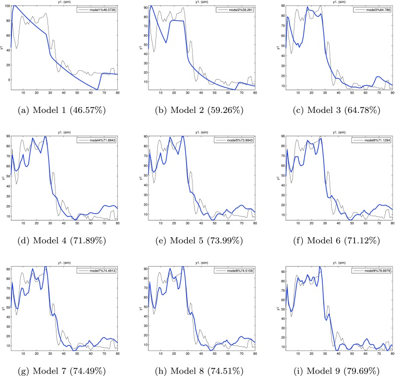
Evolution of model fit with input addition to the ARX [221] model. The percent fits for each model are shown in parenthesis. No significant improvement in model fit is obtained beyond Model 5

Table 1.

Model parameter tabulation corresponding to the drug-FM input–output pair for different multi-input models for a participant from the pilot study

Model	%fit	AIC	K p, τ, ζ, τ a	T r (days)	T s (days)
1	46.5	3.64	−12.03, 5.67, 4.14, 21.3	75.5	139.69
2	59.2	3.58	−0.91, 3.5, 2.67, 44.4	0.43	75.06
3	64.7	3.54	−1.02, 2.09, 1.5, 15.3	0.43	25.6
4	71.8	3.42	−3.11, 1.62, 1.24, 0.22	7.53	14.38
5	73.9	3.44	−2.47, 1.57, 1.26, 1.96	5.12	11.49

AIC Akaike information criterion, T _r the rise time (the time at which the response reaches 90 % of the steady state for the first time), T _s the 98 % settling time (the time at which the response reaches 98 % of its steady-state value)

Table 2 summarizes the model parameters for all inputs (manipulated and disturbance) for the Model 5 structure. The positive gain for the placebo input indicates that for this participant, pain symptoms worsened when placebo was administered. The large magnitude of the placebo gain is partly a consequence of how the input signal is coded (1 when present and 0 when not). Examining the gains for the measured disturbance models (anxiety, stress, and mood), these correspond to 0.86, 2.29, and −0.091, respectively. The positive values for the anxiety and stress gains and negative value for mood agree with the clinical observations that increases in anxiety and stress and decrease in mood should worsen FM symptoms. Table 2 also includes the model relating the effect of naltrexone on sleep. The positive gain in this model demonstrates improved sleep quality in this participant as a result of treatment. The rise and settling times associated with the sleep outcome are approximately 37 % longer than those for general FM symptoms, which implies that sleep benefits lag general FM symptom improvements.

Table 2.

Model parameter tabulation for various input-FM models for a participant from the pilot study as per Model 5. The estimated gain for the drug-FM model is negative, implying that a reduction in pain symptoms with the introduction of drug, while the gain for placebo-FM model is positive, implying worsening outcomes as a result of placebo. The table includes the case of the drug-sleep model, where the use of drug improves sleep quality

Model	K p, τ, ζ, τ a	T r (days)	T s (days)
Drug-FM	−2.47, 1.57, 1.26, 1.96	5.12	11.49
Placebo-FM	45.81, 1.57, 1.26, 1.15	6.59	13.06
Anxiety-FM	0.86, 1.57, 1.26, 0.24	7.45	14.24
Stress-FM	2.29,1.57, 1.26, 0.49	7.31	13.94
Mood-FM	−0.091, 1.57, 1.26, 4.67	0.8	11.93
Drug-OSleep	4.98, 2.13, 1.04, −3.35	7.06	15.83

Dynamic modeling for behavioral interventions: beyond black box approaches

In earlier sections, we described an empirical “black box” modeling approach for determining the process dynamics associated with the fibromyalgia intervention where the choice of the model structure has been primarily driven by aspects of goodness-of-fit and overparameterization of clinical data. However, it is possible and in many instances desirable to incorporate theories from behavioral science in a dynamical systems framework relevant to interventions [40, 41]. The interested reader is directed to work using the theory of planned behavior (TPB) to develop a dynamic model for a behavioral intervention for weight loss [20]; meanwhile, the combination of TPB and self-regulation to model the dynamics of an adaptive intervention for gestational weight gain is explored in [21–24]. The use of self-regulation for modeling smoking cessation dynamics is explored in [25–28], while a dynamical model for social cognitive theory (SCT) in the context of improving physical activity interventions is described in [41].

“CLOSED-LOOP” BEHAVIORAL INTERVENTIONS USING CONTROL SYSTEMS ENGINEERING

We noted in the “INTRODUCTION” that the ultimate goal of this research is to accomplish closed-loop treatment in which the control system assigns appropriate dosage magnitudes automatically over time. Control systems are used widely in industrial practice to achieve desired behavior of a system by systematically adjusting manipulated variables based on measured system information [4, 29, 42]. Prior work [8] has established that time-varying adaptive interventions featuring repeated assessments, intensive data, and frequent decision-making can be conceptualized as engineering control systems. In a control engineering approach to adaptive interventions, the controller assigns dosages to each participant as dictated by the solution of a formal optimization problem which fully incorporates the parameters or predictions from a dynamical model. The optimization problem is solved taking into account clinical constraints and relies on measurements (of both outcomes of interest and symptoms reports, collectively known as tailoring variables) provided by or assessed from the participant.

To conceptually illustrate this adaptive treatment strategy, the open-loop dynamical system shown in Fig. 1 is extended by “closing” the loop using a controller. In the block diagram shown in Fig. 5, P represents the dynamics expected of the treatment intervention on outcomes of interest; this is the same block as in Fig. 1. The controller, represented by the symbol C (which is part of the decision algorithm and does not represent the clinician) is supplied with clinical constraints and a cost function providing a performance metric for the optimization problem. Based on the discrepancy between the measured outcomes y (e.g., pain reports) and their desired reference values and the values of current and future symptom reports (as predicted by the model), the controller assigns dosages u to achieve a closed-loop response for each participant [8, 30]. The closed-loop control system aims at performing the following three functional tasks:

1. Reaching a desired goal (setpoint tracking). Treatment dosages are assigned to move an outcome of interest (such as pain report or sleep quality) to a desired goal. For example, the clinician may decide on a goal of 45 % reduction in the general pain symptoms report within 2 weeks of the start of the intervention.

2. Known symptoms handling (measured disturbance rejection). The controller manipulates treatment dosages to mitigate the effect from reported or assessed external influences (e.g., anxiety in case of FM intervention) using estimated disturbance models. For instance, if some external event that leads to stress or anxiety is known a priori, then dosages can be adjusted to compensate for this disturbance. It should be noted that the control engineering approach does not preclude providing the participant with a separate intervention that directly targets anxiety. However, as no treatment is perfect, if changes in anxiety levels lead to changes in FM symptoms, then it makes sense to include this information as a feedforward adjustment in the control system. The control algorithm possesses the functionality to allow this feature to be eliminated or “detuned” (as discussed later in the paper).

3. Unknown symptoms handling (unmeasured disturbance rejection). The controller can adjust treatment dosages to mitigate the effect of unknown or unmodeled external influences. For example, there could be an increase in a pain report that may not be directly associated with a change in a measured or reported condition (such as stress or anxiety). In such cases, the controller through the process of feedback compensation is able to adjust dosages to mitigate the effects of this unmeasured disturbance.

Fig 5.

Conceptual “block diagram” representation of a control system showcasing a closed-loop treatment strategy using a desired reference for a designated cost function and clinical constraints. This figure extends the concept introduced in Fig. 1 by “closing the loop.” The dosages u are assigned by the controller C based on cost function and clinical constraints to take outcomes to a desired reference setpoint or goal

The three functional modes of the control system have to be achieved under a number of practical clinical requirements, and hence, this functionality has to be integrated into the controller design. In clinical practice, treatment dosage limits are often set to minimize adverse effects, such as drug toxicity. In addition, treatment dosages are generally categorical in nature. For example, counseling sessions can either be weekly, bi-weekly, or monthly. Similarly, drug dosages are compounded in standard dosage concentration, and subsequent increase in the dosage can be prescribed as an integer multiple of that basic dose (for example, a commercially produced drug may be available only in 100, 150, and 300 mg dosages). These dosage limits are factored into the control algorithm. Furthermore, dosage changes should not be very abrupt due to potential negative consequences that the participant may experience. Hence, the controller should be tuned in such a way that dosing can be varied from a more aggressive case, where treatment dosages change rapidly over a relatively short period of time, to a more conservative case where treatment dosages change relatively slowly over time.

Model predictive control

In this work, we describe MPC as the algorithmic framework for making systematic dosage assignments. MPC has widespread application in industry, ranging from chemical process control to aerospace engineering [43]. This control technology has also been useful in designing treatment regimens for diverse medical applications, from diabetes mellitus control to HIV/AIDS treatment [16, 44–47].

Figure 6 depicts the “receding horizon” strategy that is the basis for the model predictive control algorithm. The predicted change in FM symptom severity over time (calculated using the estimated models from system identification) with prediction of measured variables like anxiety (if available) determines an error projection which shows actual and expected deviations in symptoms from the goal. On the basis of this error projection, the optimizer chooses the sequence of future control actions which minimize the error with respect to a desired goal; this process is repeated for each sample instant. The control actions are calculated by an on-line optimization algorithm as follows: the constrained optimization problem shown in Eq. (6) is numerically solved at each time instant (e.g., daily) based on model-based prediction over a period of time (defined by the prediction horizon p) and optimal treatment dosages over a period of time (defined by the move horizon m). Instead of using all of the recommended treatment dosages, only the first of the calculated dosage is applied, with the process repeated at the next assessment period (e.g., daily) until the end of the intervention. Hence, the algorithm is able to respond to unexpected symptom changes as it systematically relies on up-to-date participant response information. In Eq. (6), the optimization objective is related to the error between the predicted values (y(k + 1), …, y(k + p)) and the reference setpoint y_r, with Q_y as a user defined weight. It is solved under constraints on the allowable minimum and maximum outcome values, input treatment dosages, and their rate of change (represented by Δu(k) = u(k) − u(k − 1)). Variables p and m correspond to the prediction horizon and the move horizon, respectively.

6

Fig 6.

Receding horizon strategy used by the model predictive control algorithm illustrated for the case of naltrexone intervention with one controlled variable (FM symptoms), one manipulated variable (naltrexone dosage), and one measured disturbance (anxiety report). Control moves (i.e., dosage change decisions) are calculated by the algorithm over a horizon and only the first control move calculated using the optimization procedure is implemented. The entire procedure is repeated at the next assessment period and continues until the end of the intervention

The solution to the optimization problem denoted in Eq. (6) is accomplished through established numerical procedures from operations research. For linear dynamical models with categorical inputs, the optimization problem in Eq. (6) is solved using a mixed integer quadratic program (MIQP). Details of the algorithm and its solution are provided in [16].

The control algorithm relies on a three degree-of-freedom (3 DoF) tuning approach to flexibly achieve desired levels of performance [48, 49]. The 3 DoF tuning methodology enables the three performance requirements associated with reaching a desired goal and known and unknown symptoms handling to be adjusted independently by varying three “knobs” represented by the parameters α_r, α_d, and f_a, respectively [16, 36, 44]. This tuning approach provides the user a flexible and intuitive method to adjust the controller so that the outputs achieve a desired speed and shape of response. In the following section, we demonstrate how the 3 DoF formulation gives the flexibility to obtain desirable participant treatment profiles over time, while accommodating clinical requirements.

Closed-loop control simulation

In this section, we demonstrate an adaptive treatment scenario on the representative participant modeled from the pilot study. For simulation purposes, we consider a version of Model 5 described previously with one manipulated variable (drug), one disturbance variable (anxiety), and one output (FM symptoms). Naltrexone dosages are assumed to be available at eight levels equally spaced between 0 and 13.5 mg. The FM symptoms variable serves as the primary outcome in the analysis, while anxiety (assumed to be reported daily by the participant) serves as the measured (or known) disturbance signal.

Figure 7 illustrates the operation of the control system for adaptive drug dosage assignment under deterministic conditions. In this simulation, we show the three functional tasks that this controller can perform: reaching a setpoint goal with dosage change and dosage changes for known and unknown symptoms. Setpoint tracking (reaching the goal) starts at day 0, while the measured disturbance (anxiety report) acts between days 20 and 40, and the unmeasured disturbance (an unknown cause resulting in an increase in reported pain) acts at day 55. The baseline value for the pain report is 50 %, and a setpoint change of magnitude −9.5 is applied at day 0 as shown by the reference line (dashed red line). The pain report reaches 95 % of the setpoint in 8 days and the final goal in 11 days. The measured anxiety report acts in such a manner that it has an effect for a limited period of time (e.g., the increase in anxiety can be attributed to some stressful event). The controller increases the drug dosages to mitigate the effect of increased anxiety, with the response reaching the setpoint in around 7 days. There is an increase in the pain report (initially), but this returns to the desired symptom baseline. When the anxiety report diminishes, the controller can correspondingly reduce dosage amounts while staying within the pain threshold level acceptable to the participant. In this way, the controller responds favorably to participant feedback by efficiently varying dosages over time. At day 55, an abrupt change in the pain report occurs due to an unmeasured disturbance (e.g., a psychosocial stressor that is unrelated to the measured symptoms). In this case, we observe that since the stressor is unknown (and hence not a part of participant model), a sudden increase in the pain report is seen to which the controller responds by increasing the drug dosage to bring back the pain level to the desired goal. The response reaches the setpoint in approximately 14 days.

Fig 7.

Deterministic simulation of adaptive closed-loop naltrexone dosage assignment by the model predictive controller using eight drug dosage levels. The controller assigns dosages to reach a target pain level while addressing the effects of known and unknown symptoms on this pilot study participant. The three tuning knobs (α _r, α _d, and f _a) are all equal to 0.5; p = 25, m = 15, Q _y = 1. To reach the desired goal (a pain report of 40.5 %), the controller assigns corresponding dosages which have to be adjusted based on the values of known and unknown symptom reports

In the 3 DoF formulation, the user/clinician can vary the magnitude of the three knobs (α_r for setpoint tracking, α_d for measured disturbance rejection, and f_a for unmeasured disturbance rejection) between 0 and 1 to reach at a desired system response. The value of the knobs determines the speed of the closed-loop response. However, a faster response may result in drug dosing being too aggressive for participant comfort; hence, a proper trade-off between the speed of response and corresponding dosage profile has to be determined based on the intervention goals. The effect of tuning changes is discussed in [16] and illustrated for this simulated intervention in more detail in [36] and [50].

The simulation in Fig. 7 considered a scenario with a deterministic disturbance. A scenario in which the disturbance is of stochastic nature (generated by an ARMA (2,1) model driven by a Gaussian noise) is shown in Fig. 8. The subplot on the top shows the time series for an unmeasured disturbance, and the corresponding figure on the bottom represents the simulation under two different tuning settings and a constant dosage. The performance of these interventions is measured by the tracking error total change in drug dosage and total amount of drug dosage consumed in the intervention Setting f_a equal to 1 results in a more aggressive control action in which the variance around the pain target is minimized, but this is accomplished at the expense of a large variation in drug dosage changes. A detuned controller with f_a equal to 0.1 reduces the variance in drug dosage changes at the expense of increased variance in the participant’s pain report as noted in Table 3. In practice, f_a must be adjusted to accomplish a desired trade-off between dosage changes and reported symptoms, as deemed acceptable by the clinician and the participant. Finally, the dosage profile under tuning f_a = 0.1 is compared with a fixed dose equal to 1.92 mg to highlight the benefits of adaptation in the presence of unmeasured disturbances. The adaptive intervention offers lower tracking error while also consuming less treatment compared to the fixed dosage case, as noted in Table 3.

Fig 8.

Simulation for an unmeasured stochastic disturbance. A simulation showing change in the FM symptoms report for an unmeasured stochastic disturbance (a) is shown for the representative pilot study participant under closed-loop control (b). The drug dosages are assigned by the model predictive controller on eight levels where the controller adjusts drug dosages to compensate for changes in the general FM symptoms reports. Based on the tuning value (f _a), the resulting drug dosage changes can vary from aggressive to conservative. The fixed dosage is set at 1.92 mg. Other controller and simulation parameters remain as in Fig. 7

Table 3.

Comparison of the performance of the intervention from the control system (f _a = 1, 0.1) with a fixed dosage of naltrexone (1.92 mg) under stochastic disturbances. The control system offers lower tracking error J _e for the cost of higher variability in drug dosage J _∆u. In comparison with a constant dosage, the case f _a = 0.1 also offers lower total drug consumption J _u

Scenario	J e	J ∆u	J u
MPC (f a = 1)	6,204	1,205.1	275.79
MPC (f a = 0.1)	9,211.3	55.791	144.64
Constant drug dosage	12,328	3.6864	170.88

In industrial practice, the robustness of a control system to modeling errors and other forms of uncertainty is an important consideration [4, 42]. In the context of this application, robustness issues arise from the statistical errors resulting from parameter estimation during system identification, the variability that may exist between participants, and changes in the model that may occur within the participant over time. Space limitations prevent us from describing these concepts in more detail, but robustness of the control system is evaluated in a series of simulated scenarios relevant to the adaptive intervention that are described in [36] and [50].

SUMMARY AND CONCLUDING THOUGHTS

In this paper, we have described how techniques from dynamical systems and control engineering can be used to achieve more efficacious treatments with increased potency by enabling adaptive behavioral interventions. In this approach, a parsimonious dynamical systems model that explains the relationship between treatment and symptoms is estimated from intensive participant data. From these estimated models, an adaptive “closed-loop” dosage assignment system can be developed. The closed-loop treatment algorithm solves a receding horizon optimization problem that effectively integrates predictions from the dynamic model with repeated assessment of participant outcomes and symptoms to accomplish a personalized, optimal dosage profile over time.

To illustrate this concept, the paper focused on an example of an adaptive intervention designed to determine appropriate dosage levels of naltrexone as a treatment for fibromyalgia. Because of a lack of understanding of fibromyalgia etiology and the absence of first-principles models, we performed a secondary data analysis to estimate parsimonious models from data available through clinical trials. A multi-input ARX model, further approximated with continuous second-order differential equation models, was used to explain the effect of drug, placebo, and other variables on symptom reports of interest. Subsequently, models from a representative participant were used by a model predictive control algorithm to systematically assign dosages in the presence of disturbances and clinical constraints. We illustrated how the controller can assign treatment dosages to reach a desired set point target and then maintain this goal under conditions that involve disturbance changes in symptoms (known and unknown). This capability was demonstrated for both deterministic and stochastic disturbances.

Although the data and illustrations in this paper relied primarily on data collected from self-reports, the methodology presented can be applied without modification to data obtained from mHealth-related technologies. Increasing advances in the computing and information technologies associated with mHealth imply that the dynamical systems and optimization methods described in this paper will become more important (and commonplace) in behavioral settings in the future. Ultimately, these improvements will allow, wherever possible, for more direct and accurate measurement of human behavior and its environment, with corresponding impact in the development of more relevant and predictive models of behavior change [6, 51].

One important consideration in extending the usefulness of these methods is the role of experimental design. Traditional population-level clinical data is generally not amenable for constructing dynamical models as these are typically designed for “static” systems and are geared toward hypothesis testing and finding treatment efficacy. There has been an increasing interest in using “n-of-1” or single subject experimental protocols; these designs are highly individualized and, hence, offer certain advantages over population-level design [52–54]. Typically, treatment dosages remain constant throughout the duration of a conventional trial, which limits the effectiveness of system identification techniques. In a system identification approach to single subject experimental design, the treatment dosage is varied over time to multiple signal levels, the changes designed to provide sufficient excitation and consequently resulting in richer information regarding the dynamics of the system. Optimization approaches come into play as the experiments must increase the information content in the data while respecting clinical constraints such as limits on treatment dosage values and the rate of change of dosages over time. The work in [50, 55] discusses such approaches in detail.

In conclusion, we envision that the concepts presented in this paper will lead to novel individualized treatments where treatment dosages can be assigned by a mobile device at the disposal of the participant. The closed-loop dosage assignment can adjust treatment dosages based on daily participant reports of outcomes of interest and by incorporating predictive behavioral theories. In this way, an optimal dosage profile for that individual could be rapidly determined without requiring office visits or substantial clinician involvement. Dynamical systems modeling and control engineering offer a rich set of theoretical tools to address various demands of practice. Ultimately, we see adaptive interventions using control engineering as a cost-effective and efficient approach for accomplishing personalized behavioral interventions.

References

- 1.Hamburg MA, Collins FS. The path to personalized medicine. N Engl J Med. 2010;363(4):301–304. doi: 10.1056/NEJMp1006304. [DOI] [PubMed] [Google Scholar]
- 2.Wellstead P, Bullinger E, Kalamatianos D, Mason O, Verwoerd M. The role of control and system theory in systems biology. Annu Rev Control. 2008;32(1):33–47. doi: 10.1016/j.arcontrol.2008.02.001. [DOI] [Google Scholar]
- 3.Collins LM, Murphy SA, Bierman KL. A conceptual framework for adaptive preventive interventions. Prev Sci. 2004;5:185–196. doi: 10.1023/B:PREV.0000037641.26017.00. [DOI] [PMC free article] [PubMed] [Google Scholar]
- 4.Åström K, Murray R. Feedback Systems: An Introduction for Scientists and Engineers. Princeton: Princeton University Press; 2009. [Google Scholar]
- 5.Chakraborty B, Murphy SA. Dynamic treatment regimes. Annu Rev Stat Appl. 2014;1(1):447–464. doi: 10.1146/annurev-statistics-022513-115553. [DOI] [PMC free article] [PubMed] [Google Scholar]
- 6.Riley WT, Rivera DE, Atienza AA, Nilsen W, Allison SM, Mermelstein R. Health behavior models in the age of mobile interventions: are our theories up to the task? Transl Behav Med. 2011;1:53–71. doi: 10.1007/s13142-011-0021-7. [DOI] [PMC free article] [PubMed] [Google Scholar]
- 7.Rivera DE. Optimized behavioral interventions: what does system identification and control engineering have to offer? In: Proceedings of 16th IFAC Symposium on System Identification; 2012: 882–893.
- 8.Rivera DE, Pew MD, Collins LM. Using engineering control principles to inform the design of adaptive interventions: a conceptual introduction. Drug Alcohol Depend. 2007;88(Supplement 2):S31–S40. doi: 10.1016/j.drugalcdep.2006.10.020. [DOI] [PMC free article] [PubMed] [Google Scholar]
- 9.Zafra-Cabeza A, Rivera DE, Collins LM, Ridao MA, Camacho EF. A risk-based model predictive control approach to adaptive interventions in behavioral health. IEEE Trans Control Syst Technol. 2011;19(4):891–901. doi: 10.1109/TCST.2010.2052256. [DOI] [PMC free article] [PubMed] [Google Scholar]
- 10.Boissevain MD, McCain GA. Toward an integrated understanding of fibromyalgia syndrome. I. Medical and pathophysiological aspects. Pain. 1991;45(3):227–238. doi: 10.1016/0304-3959(91)90047-2. [DOI] [PubMed] [Google Scholar]
- 11.Younger J, Mackey S. Fibromyalgia symptoms are reduced by low-dose naltrexone: a pilot study. Pain Med. 2009;10(4):663–672. doi: 10.1111/j.1526-4637.2009.00613.x. [DOI] [PMC free article] [PubMed] [Google Scholar]
- 12.Younger J, Noor N, McCue R, Mackey S. Low-dose naltrexone for the treatment of fibromyalgia: findings of a small, randomized, double-blind, placebo-controlled, counterbalanced, crossover trial assessing daily pain levels. Arthritis Rheum. 2013;65(2):529–538. doi: 10.1002/art.37734. [DOI] [PubMed] [Google Scholar]
- 13.Ljung L. System Identification: Theory for the User. 2. Upper Saddle River: Prentice Hall; 1999. [Google Scholar]
- 14.Molenaar P, Campbell C. The new person-specific paradigm in psychology. Curr Dir Psychol Sci. 2009;18:112–117. doi: 10.1111/j.1467-8721.2009.01619.x. [DOI] [Google Scholar]
- 15.Velicer W. Applying idiographic research methods: two examples. In: Proceedings of the 8th International Conference on Teaching Statistics; 2010.
- 16.Nandola NN, Rivera DE. An improved formulation of hybrid model predictive control with application to production-inventory systems. IEEE Trans Control Syst Technol. 2013;21(1):121–135. doi: 10.1109/TCST.2011.2177525. [DOI] [PMC free article] [PubMed] [Google Scholar]
- 17.Pina AA, Holly LE, Zerr AA, Rivera DE. A personalized and control systems engineering conceptual approach to target childhood anxiety in the contexts of cultural diversity. J Clin Child Adolesc Psychol. 2014;43(3):442–453. doi: 10.1080/15374416.2014.888667. [DOI] [PMC free article] [PubMed] [Google Scholar]
- 18.Davison DE, Vanderwater R, Zhou K. A control-theory reward-based approach to behavior modification in the presence of social-norm pressure and conformity pressure. In: Proceedings of the 2012 American Control Conference; 2012: 4076–4052.
- 19.Hekler EB, Buman MP, Poothakandiyil N, Rivera DE, Dzierzewski JM, Aiken Morgan A, McCrae CS, Roberts BL, Marsiske M, Giacobbi PR. Exploring behavioral markers of long-term physical activity maintenance: a case study of system identification modeling within a behavioral intervention. Health Educ Behav. 2013;40(1 suppl):51S–62S. doi: 10.1177/1090198113496787. [DOI] [PMC free article] [PubMed] [Google Scholar]
- 20.Navarro-Barrientos JE, Rivera DE, Collins LM. A dynamical model for describing behavioural interventions for weight loss and body composition change. Math Comput Model Dyn Syst. 2011;17(2):183–203. doi: 10.1080/13873954.2010.520409. [DOI] [PMC free article] [PubMed] [Google Scholar]
- 21.Dong Y, Rivera DE, Thomas DM, Navarro-Barrientos JE, Downs DS, Savage JS, Collins LM. A dynamical systems model for improving gestational weight gain behavioral interventions. In: Proceedings of the 2012 American Control Conference; 2012: 4059–4064. [DOI] [PMC free article] [PubMed]
- 22.Dong Y, Rivera DE, Downs DS, Savage JS, Thomas DM, Collins LM. Hybrid model predictive control for optimizing gestational weight gain behavioral interventions. In: Proceedings of the 2013 American Control Conference; 2013: 1973–1978. [DOI] [PMC free article] [PubMed]
- 23.Savage JS, Downs DS, Dong Y, Rivera DE. Control systems engineering for optimizing a prenatal weight gain intervention to regulate infant birth weight. Am J Public Health. 2014;104(7):1247–1254. doi: 10.2105/AJPH.2014.301959. [DOI] [PMC free article] [PubMed] [Google Scholar]
- 24.Dong Y, Deshpande S, Rivera DE, Downs DS, Savage JS. Hybrid model predictive control for sequential decision policies in adaptive behavioral interventions. In: Proceedings of the 2014 American Control Conference; 2014: 4198–4203. [DOI] [PMC free article] [PubMed]
- 25.Timms KP, Rivera DE, Collins LM, Piper ME. A dynamical systems approach to understanding self-regulation in smoking cessation behavior change. Nicotine Tob Res. 2014;16(Suppl 2):S159–S168. doi: 10.1093/ntr/ntt149. [DOI] [PMC free article] [PubMed] [Google Scholar]
- 26.Timms KP, Rivera DE, Collins LM, Piper ME. Continuous-time system identification of a smoking cessation intervention. Int J Control. 2014;87(7):1423–1437. doi: 10.1080/00207179.2013.874080. [DOI] [PMC free article] [PubMed] [Google Scholar]
- 27.Timms KP, Rivera DE, Piper ME, Collins LM. A hybrid model predictive control strategy for optimizing a smoking cessation intervention. In: Proceedings of the 2014 American Control Conference; 2014: 2389–2394. [DOI] [PMC free article] [PubMed]
- 28.Trail JB, Collins LM, Rivera DE, Li R, Piper ME, Baker TB. Functional data analysis for dynamical system identification of behavioral processes. Psychol Methods. 2014;19(2):175–187. doi: 10.1037/a0034035. [DOI] [PMC free article] [PubMed] [Google Scholar]
- 29.Ogata K. Modern Control Engineering. Upper Saddle River: Prentice Hall; 2001. [Google Scholar]
- 30.Ogunnaike BA, Ray WH. Process Dynamics, Modeling, and Control. Oxford: Oxford University Press; 1994. [Google Scholar]
- 31.Wolfe F, Clauw D, Fitzcharles M, et al. The American College of Rheumatology preliminary diagnostic criteria for fibromyalgia and measurement of symptom severity. Arthritis Care Res. 2010;62:600–610. doi: 10.1002/acr.20140. [DOI] [PubMed] [Google Scholar]
- 32.Wolfe F, Smythe HA, Yunus M, et al. The American College of Rheumatology 1990 criteria for the classification of fibromyalgia: report of the multicenter criteria committee. Arthritis Rheum. 1990;33:160–172. doi: 10.1002/art.1780330203. [DOI] [PubMed] [Google Scholar]
- 33.Perrot S. Fibromyalgia syndrome: a relevant recent construction of an ancient condition? Curr Opin Support Palliat Care. 2008;2(2):122–127. doi: 10.1097/SPC.0b013e3283005479. [DOI] [PubMed] [Google Scholar]
- 34.Lee YC, Nassikas NJ, Clauw DJ. The role of the central nervous system in the generation and maintenance of chronic pain in rheumatoid arthritis, osteoarthritis and fibromyalgia. Arthritis Res Ther. 2011;13(2):211. doi: 10.1186/ar3306. [DOI] [PMC free article] [PubMed] [Google Scholar]
- 35.Mattiloi TM, Milne B, Cahill C. Ultra-low dose naltrexone attenuates chronic morphine-induced gliosis in rats. Mol Pain. 2010;6(22):1–11. doi: 10.1186/1744-8069-6-22. [DOI] [PMC free article] [PubMed] [Google Scholar]
- 36.Deshpande S. A control engineering approach for designing an optimized treatment plan for fibromyalgia. Master’s thesis, Electrical Engineering, Arizona State University, USA; 2011. [DOI] [PMC free article] [PubMed]
- 37.Gevers M, Miskovic L, Bonvin D, Karimi A. Identification of multi-input systems: variance analysis and input design issues. Automatica. 2006;42(4):559–572. doi: 10.1016/j.automatica.2005.12.017. [DOI] [Google Scholar]
- 38.The Mathworks. System Identification Toolbox, MATLAB User Manual for version R2009b; 2009.
- 39.Garnier H, Young PC. The advantages of directly identifying continuous-time transfer function models in practical applications. Int J Control. 2014;87(7):1319–1338. doi: 10.1080/00207179.2013.840053. [DOI] [Google Scholar]
- 40.Hekler EB, Klasnja P, Froehlich JE, Buman MP. Mind the theoretical gap: Interpreting, using, and developing behavioral theory in HCI research. In: Proceedings of the SIGCHI Conference on Human Factors in Computing Systems, CHI ’13; 2013: 3307–3316.
- 41.Martin CA, Rivera DE, Riley WT, Hekler EB, Buman MP, Adams MA, King AC. A dynamical systems model of social cognitive theory. In: Proceedings of the 2014 American Control Conference; 2014: 2407–2412.
- 42.Skogestad S, Postlethwaite I. Multivariable Feedback Control: Analysis and Design. Hoboken: Wiley; 1996. [Google Scholar]
- 43.Qin SJ, Badgwell TA. A survey of industrial model predictive control technology. Control Eng Pract. 2003;11(7):733–764. doi: 10.1016/S0967-0661(02)00186-7. [DOI] [Google Scholar]
- 44.Deshpande S, Nandola NN, Rivera DE, Younger J. A control engineering approach for designing an optimized treatment plan for fibromyalgia. In: Proceedings of the 2011 American Control Conference; 2011: 4798–4803. [DOI] [PMC free article] [PubMed]
- 45.Lee H, Buckingham B, Wilson D, Bequette B. A closed-loop artificial pancreas using model predictive control and a sliding meal size estimator. J Diabetes Sci Tech. 2009;3(5):1082–1090. doi: 10.1177/193229680900300511. [DOI] [PMC free article] [PubMed] [Google Scholar]
- 46.Wang Y, Dassau E, Doyle F. Closed-loop control of artificial pancreatic β-cell in type 1 diabetes mellitus using model predictive iterative learning control. IEEE Trans Biomed Eng. 2010;57(2):211–219. doi: 10.1109/TBME.2009.2024409. [DOI] [PubMed] [Google Scholar]
- 47.Zurakowski R, Teel AR. A model predictive control based scheduling method for HIV therapy. J Theor Biol. 2006;238(2):368–382. doi: 10.1016/j.jtbi.2005.05.004. [DOI] [PubMed] [Google Scholar]
- 48.Lee JH, Yu ZH. Tuning of model predictive controllers for robust performance. Comput Chem Eng. 1994;18(1):15–37. doi: 10.1016/0098-1354(94)85020-8. [DOI] [Google Scholar]
- 49.Wang W, Rivera DE. Model predictive control for tactical decision-making in semiconductor manufacturing supply chain management. IEEE Trans Control Syst Technol. 2008;16(5):841–855. doi: 10.1109/TCST.2007.916327. [DOI] [Google Scholar]
- 50.Deshpande S. Optimal input signal design for data-centric identification and control with applications to behavioral health and medicine. Ph.D. thesis, Electrical Engineering, Arizona State University, USA; 2014.
- 51.Nilsen W, Pavel M. Moving behavioral theories into the 21st century: technological advancements for improving quality of life. IEEE Pulse. 2013;4(5):25–28. doi: 10.1109/MPUL.2013.2271682. [DOI] [PubMed] [Google Scholar]
- 52.Hersen M, Barlow DH. Single-Case Experimental Designs: Strategies for Studying Behavior Change. Oxford: Pergamon; 1976. [Google Scholar]
- 53.Lillie EO, Patay B, Diamant J, Issell B, Topol EJ, Schork NJ. The n-of-1 clinical trial: the ultimate strategy for individualizing medicine? Personal Med. 2011;8(2):161–173. doi: 10.2217/pme.11.7. [DOI] [PMC free article] [PubMed] [Google Scholar]
- 54.Dallery J, Cassidy RN, Raiff BR. Single-case experimental designs to evaluate novel technology-based health interventions. J Med Internet Res. 2013;15(2):1–17. doi: 10.2196/jmir.2227. [DOI] [PMC free article] [PubMed] [Google Scholar]
- 55.Deshpande S, Rivera DE, Younger J. Towards patient-friendly input signal design for optimized pain treatment interventions. In: Proceedings of the 16th IFAC Symposium on System Identification; 2012: 1311–1316.