BADGE: A novel Bayesian model for accurate abundance quantification and differential analysis of RNA-Seq data

Abstract

Background

Recent advances in RNA sequencing (RNA-Seq) technology have offered unprecedented scope and resolution for transcriptome analysis. However, precise quantification of mRNA abundance and identification of differentially expressed genes are complicated due to biological and technical variations in RNA-Seq data.

Results

We systematically study the variation in count data and dissect the sources of variation into between-sample variation and within-sample variation. A novel Bayesian framework is developed for joint estimate of gene level mRNA abundance and differential state, which models the intrinsic variability in RNA-Seq to improve the estimation. Specifically, a Poisson-Lognormal model is incorporated into the Bayesian framework to model within-sample variation; a Gamma-Gamma model is then used to model between-sample variation, which accounts for over-dispersion of read counts among multiple samples. Simulation studies, where sequencing counts are synthesized based on parameters learned from real datasets, have demonstrated the advantage of the proposed method in both quantification of mRNA abundance and identification of differentially expressed genes. Moreover, performance comparison on data from the Sequencing Quality Control (SEQC) Project with ERCC spike-in controls has shown that the proposed method outperforms existing RNA-Seq methods in differential analysis. Application on breast cancer dataset has further illustrated that the proposed Bayesian model can 'blindly' estimate sources of variation caused by sequencing biases.

Conclusions

We have developed a novel Bayesian hierarchical approach to investigate within-sample and between-sample variations in RNA-Seq data. Simulation and real data applications have validated desirable performance of the proposed method. The software package is available at http://www.cbil.ece.vt.edu/software.htm.

Background

Next Generation Sequencing (NGS) technology has opened a new era for transcriptome analysis, which grants the ability to investigate novel biological problems, such as alternative splicing, differential isoforms, gene fusion, etc. By piling up millions of reads along the reference genome, RNA-Seq technology can obtain signals in a much larger dynamic range with much higher accuracy compared to traditional microarray based technologies. For RNA-Seq analysis, the most popular routine is to determine the expression of genes (abundance quantification) and to identify differentially expressed genes (DEGs).

Methods that quantify gene/isoform level expression mainly fall into two categories: Poisson count mode (e.g., Cufflinks [1], etc) and linear regression model (e.g., Isolasso [2], SLIDE [3], BASIC [4], etc.). The major challenge in accurate quantification of gene expression is that large systematic bias in sequencing counts has been observed due to multiple factors. In contrast to uniform assumption of read distribution, it has been reported that sequence counts show a variety of physical and chemical biases, including transcript length bias, GC-content bias, random hexamer priming bias, etc [5-7].

Differential analysis of RNA-Seq data has been focused on modeling variance among biological replicates or samples in the same phenotype group. EdgeR [8] is the first method that models the 'between-sample' variability by replacing the Poisson model with Negative Binomial model. Various statistical methods have been proposed to model the variance among samples in biological groups, aimed to improve overall fitting of count data or robustness against outliers [9-12].

Despite initial success to model uncertainties associated with sequencing counts from different aspects, there lacks a systematic effort to address variability in RNA-Seq data. We dissect the variance in sequencing counts along two dimensions: over-dispersion of read counts within the same sample (i.e., within-sample variation) and over-dispersion of read counts among individuals from the same biological group (i.e., between-sample variation). Within-sample variation typically leads to large variance of read counts among genomic loci (e.g., nucleotides or exons), which have similar expression level in the same sample. It is typically caused by technical artifacts such as uncorrected systematic bias and gene specific random effects. On the other hand, between-sample variation is mostly due to biological differences among samples under the same condition. To increase the accuracy of abundance estimation so as to improve DEG identification, immediate attention is needed to developing a unified model that takes care of both forms of variation in RNA-Seq data. We propose a computational method, namely Bayesian Analysis of Dispersed Gene Expression ('BADGE'), to model variability in RNA-Seq data. A full Bayesian model is employed to simultaneously account for within-sample variation and between-sample variation to improve inference. The proposed method has several novel contributions compared to existing methodologies: 1) a unified Bayesian causality model is developed for joint abundance estimation and DEG identification. The improved accuracy in profiling mRNA abundance can facilitate the identification of DEGs, which may in turn refine the parameter learning in abundance quantification. 2) A Poisson-Lognormal regression model is incorporated to model within-sample variation [13]. Instead of dealing with multiples sources of technical bias and variation separately, the proposed method can 'blindly' detect over-dispersion pattern within the individual sample. 3) Gamma-Gamma model [14] is used to model between-sample variation, which accounts for over-dispersion of read counts among multiple samples. BADGE is a unified computational method that extensively models variability in RNA-seq data to improve abundance quantification and DEG identification.

Methods

Bayesian Analysis of Dispersed Gene Expression (BADGE)

We have developed a computational method, namely Bayesian Analysis of Dispersed Gene Expression (BADGE), to model extensive variability in RNA-Seq data. BADGE explicitly models both between-sample variation and within-sample variation to improve abundance quantification and DEG identification. In this paper, we only focus on the gene level analysis, while the concept can be straight-forwardly generalized for genes with multiple transcripts (isoforms).

Let y_g,i,j represent observed counts that fall into the i^th (1 ≤ i ≤ I_g) exon region of gene g (1 ≤ g ≤ G) in sample j (1 ≤ j ≤ J), which follows Poisson distribution with mean γ_g,i,j. I_g is the number of exons in gene g. G is the total number of genes. J = J₁ + J₂ is the total number of samples, where J₁ and J₂ denote samples in condition 1 and 2, respectively. Within-sample over-dispersion indicates that γ_g,i,j has unknown heterogeneity across the gene rather than taking constant value. A hierarchical Bayesian model is constructed to model within-sample variation of RNA-Seq data as follows:

$$y_{g,i,j}~Poiss\left({\gamma }_{g,i,j}\right),$$ (1)

$${\gamma }_{g,i,j}=x_{g,i}{\beta }_{g,j}\text{exp}\left(U_{g,i,j}\right),$$ (2)

$$U_{g,i,j}~N\left(0,\tau \right),\text{s}\text{.t}\text{.}{\displaystyle \sum _i}{U}_{g,i,j}=0,$$ (3)

$$\tau ~Gamma\left(a,b\right),$$ (4)

where β_g,j is the true expression level of gene g for sample j. x_g,i is the length of the i^th exon weighted by the library size of sample j. U_g,i,j is the unknown within-sample variation parameter, which follows normal distribution with mean 0 and precision τ. 'Flat' prior is assigned for τ by setting its shape a = 1 and rate b = 0. Equations (1-4) are also known as the Poisson-Lognormal regression model with identity link function.

Not only does the read count y_g,i,j exhibits over-dispersion, but also β_g,j has variation across multiple samples in the same biological group. To model between-sample variation carried by β_g,j, we adopt the Gamma-Gamma model that is widely used in microarray gene expression analysis [14] into the Poisson count model. Let j₁ and j₂ represent samples in condition 1 and 2. d_g is the binary differential state of gene g, where d_g = 0 means gene g is not differentially expressed; d_g = 1, otherwise. The Gamma-Gamma model for RNA-Seq differential expression is given by:

$$\text{If}{d}_g=0,{\beta }_{g,j}~Gamma\left(\alpha ,{\lambda }_g\right),$$ (5)

$${\lambda }_g~Gamma\left({\alpha }_0,v\right),$$ (6)

$$\text{or}\text{if}dg=1,{\beta }_{g,j_1}~Gamma\left(\alpha ,{\lambda }_{{}_g}^{\left(1\right)}\right),{\beta }_{g,j_1}~Gamma\left(\alpha ,{\lambda }_{{}_g}^{\left(2\right)}\right)$$ (7)

$${\lambda }_g^{\left(1\right)},{\lambda }_g^{\left(2\right)}~Gamma\left({\alpha }_0,v\right),$$ (8)

$$\text{and}v~Gamma\left(a_0,b_0\right),$$ (9)

where ${\lambda }_g^{\left(1\right)}$ and ${\lambda }_g^{\left(2\right)}$ are the rate parameters of Gamma distribution. If d_g = 0, ${\lambda }_g^{\left(1\right)}={\lambda }_g^{\left(2\right)}={\lambda }_g$; if $d_g=1,{\lambda }_g^{\left(1\right)}\ne {\lambda }_g^{\left(2\right)}$. α is the shape parameter for β_g,j, which does not depend on differential state d_g Moreover, we assume that the pooled rate parameter λ_g from the gene population further follows Gamma distribution with shape parameter α₀ and rate parameter v. We assign non-informative priors for hyper-parameters α, α₀, d_g(P(d_g = 1)= π_g = 0.5) and v(a₀ = 1, b₀ = 0). The sub-model defined by Equations (5-9) considers between-sample variation within the same group, which borrows knowledge from the entire population to improve parameter estimation of individual genes. Figure 1 gives the Bayesian hierarchical dependency graph for all the parameters involved in the BADGE method using plate notation. There are three plates in Figure 1: The inner plate denotes dependency among read counts within I_g exons in gene g; middle plate denotes dependency among J samples; and the outmost plate represents G genes. Observation y, represented by shaded circle, is the raw exon level RNA-Seq count (for gene level count data, I_g = 1), which depends on mRNA abundance β, gene design matrix x and within-sample over-dispersion parameter U. β further depends on group level between-sample over-dispersion Gamma parameter λ and α, and U depends on global within-sample over-dispersion parameter τ. Parameter λ is determined by gene level differential state d, and its priors ν and α₀. d_g (differential state of gene g) is assumed to follow P(dg = 1) = π_g = 0.5. Hyper-parameters a₀, b₀, π, a, and b, shown in shaded square, are fixed to construct non-informative priors (see additional file 1).

Figure 1.

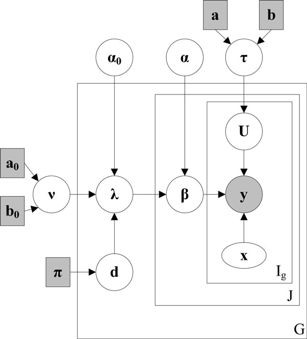
Dependency graph of model parameters in BADGE.Observation (read count) y is shaded, while the random variables are denoted as circles. Fixed parameters are denoted as shaded squares. Exon length information x is denoted as oval. I_g is the number of exons, J is the total number of samples in two groups, and G is the number of genes. Note that parameter λ actually is a parameter set {λ⁽¹⁾, λ⁽²⁾}, which correspond to two sample conditions.

Estimate model parameters using Gibbs sampling

The joint posterior distribution of all parameters given observation y (read count) and x (exon length) is given by:

$$\begin{array}{c}P\left(\beta ,U,\tau ,\lambda ,d,\alpha ,{\alpha }_0,v|y,x\right)\hfill \\ ~P\left(y|\beta ,U,\tau ,\lambda ,d,\alpha ,{\alpha }_0,v,x\right)P\left(\beta ,U,\tau ,\lambda ,d,\alpha ,{\alpha }_0,v|x\right)\hfill \\ ~P\left(y|\beta ,x,U,\tau ,\right)P\left(U|\tau \right)P\left(\beta |\lambda ,\alpha \right)P\left(\lambda |d,{\alpha }_0,v\right)P\left(\tau \right)P\left(d\right)P\left(\alpha \right)P\left({\alpha }_0\right)P\left(v\right)\hfill \\ ~\prod _g\prod _{j_1}\prod _i\left(\frac{{\left(x_{g,i}{\beta }_{{}_{g,j_1}}\text{exp}\left(U_{g,i,j_1}\right)\right)}^{y_{g,i,j_1}}}{y_{g,i,j_1}!}.e^{-x_{g,i}{\beta }_{g,j1}\text{exp}\left(U_{g,i,j_1}\right)}\right)\hfill \\ \times \prod _g\prod _{j_2}\prod _i\left(\frac{{\left(x_{g,i}{\beta }_{{}_{g,j_2}}\text{exp}\left(U_{g,i,j_2}\right)\right)}^{y_{g,i,j_2}}}{y_{g,i,j_2}!}.e^{-x_{g,i}{\beta }_{g,j_2}\text{exp}\left(U_{g,i,j_2}\right)}\right)\hfill \\ \times \prod _g\prod _j\prod _i{\sqrt{\tau e}}^{-\tau \frac{U_{g,i,j}^2}{2}}\hfill \\ \times \prod _g\left(\prod _{j_1}\frac{{\left({\lambda }_g^{\left(1\right)}\right)}^{\alpha }}{\text{Γ}\left(\alpha \right)}{\beta }_{g,j_1}^{\alpha -1}{e}^{-{\lambda }_g^{\left(1\right)}{\beta }_{g,j_1}}\times \prod _{j_2}\frac{{\left({\lambda }_g^{\left(2\right)}\right)}^{\alpha }}{\text{Γ}\left(\alpha \right)}{\beta }_{g,j_2}^{\alpha -1}{e}^{-{\lambda }_g^{\left(2\right)}{\beta }_{g,j_{{}_2}}}\right)\hfill \\ \times \prod _g{\left(\frac{v^{{\alpha }_0}}{\text{Γ}\left({\alpha }_0\right)}{\left({\lambda }_g^{\left(1\right)}\right)}^{{\alpha }_0-1}{e}^{-v{\lambda }_g^{\left(1\right)}}\times \frac{v^{{\alpha }_0}}{\text{Γ}\left({\alpha }_0\right)}{\left({\lambda }_g^{\left(2\right)}\right)}^{{\alpha }_0-1}{e}^{-v{\lambda }_g^{\left(2\right)}}\right)}^{d_g}\hfill \\ \times \prod _g{\left[\frac{v^{{\alpha }_0}}{\text{Γ}\left({\alpha }_0\right)}{\left({\lambda }_g^{\left(1\right)}\right)}^{{\alpha }_0-1}{e}^{-v{\lambda }_g^{\left(1\right)}}\times \text{I}\left({\lambda }_g^{\left(1\right)}-{\lambda }_g^{\left(2\right)}\right)\right]}^{1-d_g}\hfill \\ \times \frac{b^a}{\text{Γ}\left(a\right)}{\tau }^{a-1}{e}^{-b\tau }\times \prod _g{\pi }_g\times \frac{b_0^{a_0}}{\text{Γ}\left(a_0\right)}{v}^{a_0-1}{e}^{-b_{0}v},\hfill \\ \hfill \end{array}$$ (10)

For Poisson-Lognormal regression model, the posterior distributions of parameters β_g,j, U_g,i,j and τ can be sampled from their corresponding conditional distributions as:

$$\begin{array}{c}P\left({\beta }_{g,j}|y,U_g\right)~{\beta }_{g,j}^{{\displaystyle \sum _i}{y}_{g,i,j}}\left(-{\beta }_{g,j}{\displaystyle \sum _i}{x}_{g,i}\text{exp}\left(U_{g,i,j}\right)\right)\\ ~Gamma\left({\displaystyle \sum _i}{y}_{g,i,j}+1,{\displaystyle \sum _i}{x}_{g,i}\text{exp}\left(U_{g,i,j}\right)\right),\\ \end{array}$$ (11)

$$P\left(U_{g,i,j}|{\beta }_{g,j},\tau ,y\right)~\text{exp}{\left(U_{g,i,j}\right)}^{y_{g,i,j}}\times \text{exp}\left(-{\beta }_{g,j}{x}_{g,i}\text{exp}\left(U_{g,i,j}\right)\right)\times \text{exp}\left(-\frac{\tau U_{g,i,j}^2}{2}\right),$$ (12)

$$\begin{array}{c}P\left(\tau |U\right)~{\tau }^{a-1+\frac{J{\displaystyle \sum _g}{I}_g}{2}}\times \text{exp}\left(-\left(b+{\displaystyle \sum _{g,i,j}}\frac{U_{g,i,j}^2}{2}\right)\tau \right)\\ ~Gamma\left(a+\frac{J{\displaystyle \sum _g}{I}_g}{2},b+{\displaystyle \sum _{g,i,j}}\frac{U_{g,i,j}^2}{2}\right).\\ \end{array}$$ (13)

We pool all the samples from U_g,i,j and get its estimate ${\hat{U}}_{g,i,j}=\frac{1}{T-t_b+1}{\displaystyle \sum _{t_b}^T}{U}_{g,i,j}^t,$ where $U_{g,i,j}^t$ denotes sampled U_g,i,j at sample t. t_b is the last sample when burn-in stops. T is the total number of Gibbs samples. ${\hat{U}}_{g,i,j}$ will be passed to the Gamma-Gamma model to estimate parameters associated with DEG identification.

Similarly for the Gamma-Gamma model, we sample the parameters β, λ, α, α₀, v and d according to their conditionals. The posterior distribution of ${\beta }_j\left({\beta }_{j_1},{\beta }_{j_2}\right)$ can be sampled from:

$$\text{P}\left({\beta }_{g,j_1}|y_{g,j_1},{\lambda }_g^{\left(1\right)},\alpha \right)~Gamma\left({\displaystyle \sum _i}{y}_{g,i,j_1}+\alpha ,{\displaystyle \sum _i}{x}_{g,i}\text{exp}\left({\hat{U}}_{g,i,j_1}\right)+{\lambda }_g^{\left(1\right)}\right),$$ (14)

$$\text{P}\left({\beta }_{g,j_2}|y_{g,j_2},{\lambda }_g^{\left(2\right)},\alpha \right)~Gamma\left({\displaystyle \sum _i}{y}_{g,i,j_2}+\alpha ,{\displaystyle \sum _i}{x}_{g,i}\text{exp}\left({\hat{U}}_{g,i,j_2}\right)+{\lambda }_g^{\left(2\right)}\right).$$ (15)

If d_g = 1,

$$\text{P}\left({\lambda }_g^{\left(1\right)}|{\beta }_g^{\left(1\right)},\nu ,\alpha ,{\alpha }_0\right)~Gamma\left(J_1\alpha +{\alpha }_0,{\displaystyle \sum _{j_1}}{\beta }_{g,j_1}+\nu \right),$$ (16)

$$\text{P}\left({\lambda }_g^{\left(2\right)}|{\beta }_g^{\left(2\right)},\nu ,\alpha ,{\alpha }_0\right)~Gamma\left(J_2\alpha +{\alpha }_0,{\displaystyle \sum _{j_2}}{\beta }_{g,j_2}+\nu \right);$$ (17)

If d_g = 0,

$$\text{P}\left({\lambda }_g^{\left(1\right)}|{\beta }_g,\nu ,\alpha ,{\alpha }_0\right)=P\left({\lambda }_g^{\left(2\right)}|{\beta }_g,\nu ,\alpha ,{\alpha }_0\right)~Gamma\left(J\alpha +{\alpha }_0,{\displaystyle \sum _j}{\beta }_{g,j}+\nu \right).$$ (18)

The posterior distribution of ν follows Gamma distribution that is given by:

$$\text{P}\left(\nu |\lambda ,\mathbf{\text{d}},\alpha ,{\alpha }_0\right)~Gamma\left(\left(G+{\displaystyle \sum _g}{d}_g\right){\alpha }_0+a_0,{\displaystyle \sum _g}\left({\lambda }_g^{\left(1\right)}+{\lambda }_g^{\left(2\right)}\times d_g\right)+b_0\right).$$ (19)

According to Wei etal. [14], the posterior distribution of d given β, α, α₀ and ν can be derived as:

$$\begin{array}{c}P\left(d_g|\beta ,\alpha ,{\alpha }_0,\nu \right)={\left(K_1{K}_2\frac{{\left({\displaystyle \prod _{j_1}}{\beta }_{g,j_1}\times {\displaystyle \prod _{j_2}}{\beta }_{g,j_2}\right)}^{\alpha -1}}{{\left(\nu +{\displaystyle \sum _{j_1}}{\beta }_{g,j_1}\right)}^{J_1\alpha +{\alpha }_0}{\left(\nu +{\displaystyle \sum _{j_2}}{\beta }_{g,j_2}\right)}^{J_2\alpha +{\alpha }_0}}\right)}^{d_g}\\ \times {\left(K\frac{{\left({\displaystyle \prod _{j_1}}{\beta }_{g,j_1}\times {\displaystyle \prod _{j_2}}{\beta }_{g,j_2}\right)}^{\alpha -1}}{{\left(\nu +{\displaystyle \sum _{j_1}}{\beta }_{g,j_1}+{\displaystyle \sum _{j_2}}{\beta }_{g,j_2}\right)}^{\left(J_1+J_2\right)\alpha +{\alpha }_0}}\right)}^{1-d_g}\times {\pi }_g,\\ \end{array}$$ (20)

where

$$K_1=\frac{{\nu }^{{\alpha }_0}\text{Γ}\left(J_1\alpha +{\alpha }_0\right)}{{\text{Γ}}^{J_1}\left(\alpha \right)\text{Γ}\left({\alpha }_0\right)},K_2=\frac{{\nu }^{{\alpha }_0}\text{Γ}\left(J_2\alpha +{\alpha }_0\right)}{{\text{Γ}}^{J_2}\left(\alpha \right)\text{Γ}\left({\alpha }_0\right)},\text{and }K=\frac{{\nu }^{{\alpha }_0}\text{Γ}\left(\left(J_1+J_2\right)\alpha +{\alpha }_0\right)}{{\text{Γ}}^{J_1+J_2}\left(\alpha \right)\text{Γ}\left({\alpha }_0\right)}.$$

The posterior distribution of α₀ and α are given by:

$$P\left({\alpha }_0|\nu ,\lambda ,\mathbf{\text{d}}\right)~{\displaystyle \prod _g}\left(\frac{{\nu }^{{\alpha }_0}}{\text{Γ}\left({\alpha }_0\right)}{\left({\lambda }_g^{\left(1\right)}\right)}^{{\alpha }_0-1}\times {\left(\frac{{\nu }^{{\alpha }_0}}{\text{Γ}\left({\alpha }_0\right)}{\left({\lambda }_g^{\left(2\right)}\right)}^{{\alpha }_0-1}\right)}^{d_g}\right),$$ (21)

$$P\left(\alpha |\beta ,\lambda \right)~{\displaystyle \prod _g}\left({\displaystyle \prod _{j_1}}\frac{\left({\lambda }_g^{\left(1\right)}\right)}{\text{Γ}\left(\alpha \right)}{\beta }_{g,j_1}^{\alpha -1}\times {\displaystyle \prod _{j_2}}\frac{{\left({\lambda }_g^{\left(2\right)}\right)}^{\alpha }}{\text{Γ}\left(\alpha \right)}{\beta }_{g,j_2}^{\alpha -1}\right).$$ (22)

We use Gibbs sampling method [4,13,15,16] to estimate the posterior distributions of individual parameters iteratively from their complex joint distribution. For parameters β, ν, τ, and λ, we use conjugate priors to sample from their conditional distributions with standard probability distributions (Gamma distribution). For parameters (U, α₀ and α) that do not have conjugate priors, we use Metropolis-Hastings sampling to sample their posterior distributions. Please see more details about the implementation of Gibbs sampler in additional file 1.

Results and discussion

Over-dispersion of RNA-Seq counts in two dimensions: between-sample variation and within-sample variation

Even though RNA-Seq has been proved to be more accurate and less sensitive to background noise than traditional microarray technology [17], large variance in sequencing counts has complicated the detection of hidden biological signals. Increasing evidence shows that read counts in RNA-Seq data have much larger variance than the mean (i.e., 'over-dispersion'), which requires replacing the Poisson model with more sophisticated count models such as Negative Binomial model [8]. Figure 2 (a) shows the scatter plot of mean versus variance for three RNA-Seq datasets: basal breast cancer samples from The Cancer Genome Atlas (TCGA) project [18], human B cell datasets from Cheung et al.[19], and a mouse dataset [20]. The slopes of the least squares (LS) fit lines for all scatter plots are apparently larger than the Poisson model, which implies severe over-dispersion in all three RNA-seq datasets. In addition to variability across samples ('between-sample variation'), we have also observed strong variance of sequencing counts among genomic loci in the same biological sample ('within-sample variability'). Figure 2 (b) shows the scatter plots of counts that fall in 100nt bins along the same gene within the same sample. One TCGA breast cancer sample and one MCF7 breast cancer cell line sample [21] are used as examples. Figure 2 (b) shows strong within-sample over-dispersion of read counts in both RNA-Seq samples, implying the presence of unknown sources of variability. Figure 2 (c) shows the variation of sequencing bias among all the genes within one sample. Despite an overall tendency where read coverage is biased towards the 3'-end of the transcript, subgroups of the genes in the genome exhibit diverse patterns showing either a bias towards the 5'-end or having depleted coverage on both ends. In Figure 2 (d), we further show an example of read coverage for gene S100A9 (exon 2) across four samples from TCGA basal breast cancer dataset. The base level coverage has two distinct patterns, indicating large variation of unknown read bias in the same group. The ambiguity in coverage pattern cannot be explained by deterministic systematic bias, and therefore need to be corrected for accurate estimation of RNA-Seq abundance.

Figure 2.

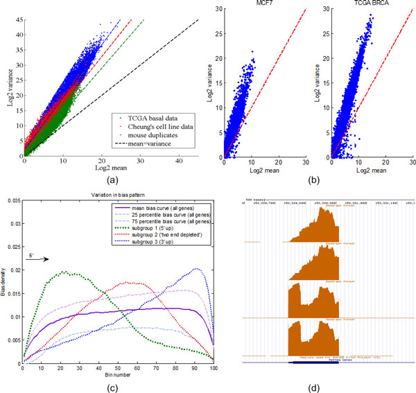
Between-sample variation and within-sample variation in RNA-Seq data.(a) Three datasets are used to show the over-dispersion of reads across samples. Scatter plots are in log 2 scale. (b) In both MCF7 breast cancer samples and TCGA breast cancer patient samples, we observe that the variance of read counts is significantly larger than the average counts in 100nt bins. (c) Bias patterns of genes in the same sample are further dissected. In contrast to a general right-tailed (biased towards 3'-end of transcript) coverage, we also observe groups of genes that have either biased expression towards the 5'-end, or depleted expression in both ends. (d) An example to show variation of sequencing bias among biological samples.

Generate simulation data based on real RNA-Seq datasets

To generate realistic synthetic data that represent characteristics of real RNA-Seq data, we adopted a simulation strategy proposed by Wu et al. [10] to first estimate model parameters from real datasets and then use them to generate sequencing counts based on human annotation file (version: GRCh37/hg19). Two RNA-Seq datasets were used in the study: 1) a mouse dataset with 10 C57BL/6J (B6) mouse samples and 11 DBA/2J (D2) mouse samples [20]; 2) 23 basal breast cancer samples from the TCGA project [18]. For the TCGA dataset, we divided the patients (which received chemotherapy treatment) into two groups: early re-current group (recurrence time < 2 yrs, 13 samples) and late recurrent group (recurrence time > 3 yrs, 10 samples). Figure 3 gives the trace plots of sampled model parameters. We used thin = 10 for the Gibbs sampling process, which means to record every 10^th sample. It took BADGE several hours to estimate posterior distributions using 10,000 iterations on real dataset. We have also plotted auto-correlation curves of each parameter in supplementary materials (additional file 1). We further explored the variability of RNA-Seq data by close examination of estimated model parameters. For within-sample variability, two typical values of over-dispersion prior parameter τ have been estimated, where τ = 0.44 in mouse dataset and τ = 1.78 in TCGA dataset. In our Poisson-Lognormal regression model, τ is the precision parameter (inverse of Gaussian variance σ²) that controls overall degree of within-sample over-dispersion. Smaller τ indicates larger variation of read counts across the transcriptome. Small value of τ observed in real datasets strongly supported our motivation that read counts along one transcript must be corrected for improved abundance estimation. Between-sample variability is jointly determined by α, α₀, and ν. Small value in ν (0.001 in mouse and 0.2 in TCGA sample) yield large variation of VAR (λ), where VAR (β) increases when λ takes small value. We used the model parameters estimated from real datasets to generate read counts for simulation. Please refer to supplementary materials in additional file 1 for more detailed description of simulation data.

Figure 3.

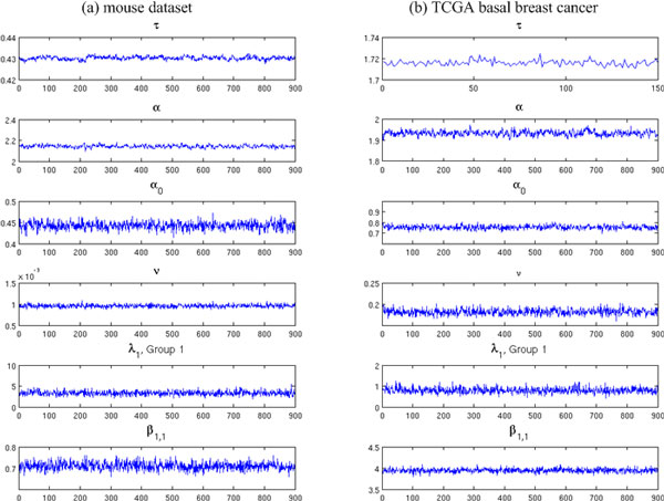
Estimate of model parameters from real datasets.(a) Model parameters estimated from mouse dataset. (b) Model parameters estimated from TCGA basal breast cancer dataset. For most parameters, we record 900 samples (thin = 10, i.e., record every 10^th sample) after the first 100 burn-in samples. An exception was made for learning parameter τ in TCGA dataset to reduce memory usage in estimating Poisson-Lognormal regression model (200 samples were recorded, among which first 50 were discarded as burn-in).

Performance comparison for abundance estimation on simulation data

We incorporated the estimated parameter τ from real datasets to generate synthetic data and studied the performance of the BADGE method for abundance estimation. We compared our method with four commonly used methods for RNA-Seq normalization, which were: reads-per-kilobase-per-million (RPKM), DESeq, trimmed mean of M-values (TMM) and upper quantile normalization (UQUA). RPKM [22] is calculated through normalizing reads by length of genomic features (genes and exons) and total library size. DESeq normalization is implemented by DESeq (1.14.1) [9], which is a differential gene identification method based on negative binomial model. TMM was originally developed in edgeR [8] and later included into BioConductor package NOISeq [23]. NOISeq (2.0.0) also has separate implementations of RPKM and UQUA methods, which were used here for performance comparison. Based on estimated parameters from real RNA-Seq datasets (mouse and TCGA breast cancer data), we selected typical model parameters to simulate count data: σ = 0.75, 1 and 1.5; ν = 0.1 and 0.001; α = 2 and α₀ = 0.5. We used the average correlation of normalized counts with ground truth gene expression to measure the accuracy of abundance quantification across multiple samples. Figure 4 gives the average correlation for all competing methods under different model settings. From Figure 4, we see that the BADGE method had robust performance under different over-dispersion settings by maintaining a performance measure (correlation to ground truth) very close to 1. Among the rest of the normalization methods, DESeq, TMM and UQUA achieved comparable performance across multiple parameter settings, while RPKM had the least favourable performance in all scenarios. Our computational result is quite consistent with the observation by Dillies et al. [24] that DESeq and TMM (edgeR) are much better normalization methods than RPKM.

Figure 4.

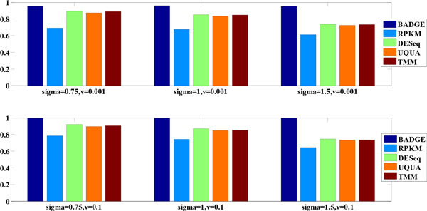
Performance comparison for abundance estimation on simulation data.

Performance comparison for differentially expressed gene (DEG) identification on simulation data

We compared BADGE with four existing methods: DESeq (1.14.1, fitType=local), edgeR (3.4.2, default), DSS (2.0.0, default), EBSeq (1.3.1, default), for differentially expressed gene (DEG) identification from RNA-Seq data. We used parameters learned from real datasets to generate simulation data. Within-sample variability is controlled by precision parameter τ (or standard deviation σ), and we set τ = 1.78 (i.e., σ = 0.75, which was learned from TCGA basal dataset) and τ = 0.44 (i.e., σ = 1.5, which was learned from mouse dataset.). According to estimated parameters from real datasets, we set α = 2, α₀ = 0.5, while varied ν between 0.001 and 0.1, which was consistent with the parameter settings in abundance estimation. For each parameter set, we randomly selected 10 genesets from hg19 annotation file to evaluate the variance of the performance. Area-under-the-curve (AUC) of the receiver operating characteristic (ROC) curve was used as performance measurement. Tables 1, 2, 3 give the AUC values for each method along with standard deviations (listed in parentheses) of AUCs across 10 experiments.

Table 1.

Performance comparison using AUC for DEG identification (highly differentially expressed genes)

σ (τ)	ν	BADGE	DESeq	edgeR	DSS	EBSeq
0.75	0.001	0.939	0.921	0.919	0.881	0.928
(1.78)		(0.018)	(0.017)	(0.018)	(0.055)	(0.017)
	0.1	0.918	0.894	0.895	0.889	0.906
		(0.018)	(0.018)	(0.020)	(0.024)	(0.021)
1.5	0.001	0.925	0.881	0.875	0.809	0.890
(0.44)		(0.014)	(0.029)	(0.032)	(0.082)	(0.030)
	0.1	0.924	0.868	0.865	0.858	0.875
		(0.023)	(0.027)	(0.025)	(0.027)	(0.022)

Table 2.

Performance comparison using AUC for DEG identification (moderately differentially expressed genes)

σ (τ)	ν	BADGE	DESeq	edgeR	DSS	EBSeq
0.75	0.001	0.901	0.724	0.753	0.739	0.750
(1.78)		(0.071)	(0.070)	(0.081)	(0.197)	(0.069)
	0.1	0.905	0.768	0.760	0.852	0.781
		(0.076)	(0.051)	(0.066)	(0.071)	(0.044)
1.5	0.001	0.882	0.691	0.699	0.790	0.725
(0.44)		(0.056)	(0.041)	(0.042)	(0.088)	(0.035)
	0.1	0.890	0.743	0.729	0.798	0.748
		(0.080)	(0.070)	(0.081)	(0.074)	(0.058)

Table 3.

Performance comparison using AUC for DEG identification (weakly differentially expressed genes)

σ (τ)	ν	BADGE	DESeq	edgeR	DSS	EBSeq
0.75	0.001	0.793	0.656	0.680	0.603	0.687
(1.78)		(0.099)	(0.058)	(0.084)	(0.133)	(0.031)
	0.1	0.778	0.659	0.663	0.695	0.684
		(0.092)	(0.043)	(0.062)	(0.075)	(0.049)
1.5	0.001	0.806	0.641	0.647	0.635	0.669
(0.44)		(0.080)	(0.028)	(0.071)	(0.134)	(0.029)
	0.1	0.823	0.687	0.680	0.724	0.682
		(0.109)	(0.072)	(0.063)	(0.104)	(0.073)

We simulated RNA-Seq gene expression with three different scenarios: genes that were highly differentially expressed, moderately differentially expressed and weakly differentially expressed (see supplementary materials in additional file 1 for more information). From Tables 1, 2, 3, we see that the BADGE method consistently outperformed existing methods in different parameter settings (highlighted in bold). For highly differentially expressed genes (Table 1), the performance of the other methods degraded as we decreased τ, while BADGE was able to maintain good performance by employing a Poisson-Lognormal model to account for within-sample variability. For genes that were weakly differentially expressed (Table 3), BADGE achieved a maximum improvement of AUC up to 1.3, compared to the second best method EBSeq (Table 3, τ = 0.44, ν = 0.001).

Performance comparison for differentially expressed gene (DEG) identification on Sequencing Quality Control (SEQC) data

We compared the performance of BADGE with existing RNA-Seq differential gene identification methods on the Sequencing Quality Control (SEQC) dataset with ERCC spike-in controls [25]. 92 artificial transcripts were mixed into a real RNA-Seq library with different ratios (1:1 for none differentially expressed genes, and 4:1, 2:3 and 1:2 for differentially expressed genes), which were used as ground truth differential states for differential gene identification. Gene level counts were downloaded from http://bitbucket.org/soccin/seqc. We compared the ROC curves between BADGE and four other methods used in the simulation study for differential gene identification, which were DESeq [9], edgeR [8], DSS [10] and EBSeq [11]. Figure 5 shows the ROC curves of the five competing methods.

Figure 5.

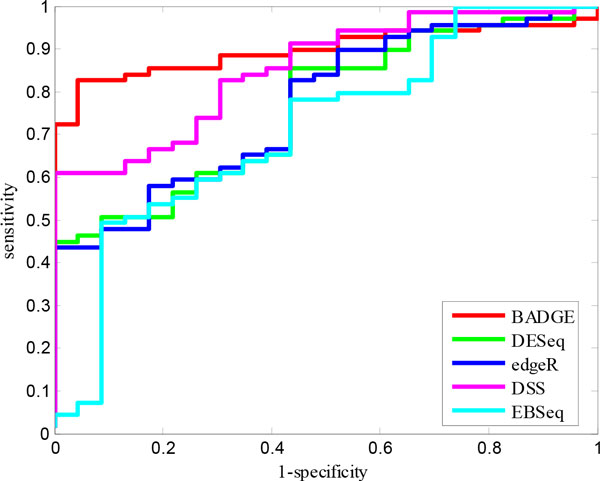
Performance comparison for differentially expressed gene identification on the SEQC dataset.

On the SEQC dataset, BADGE had the best performance among all five methods by achieving an AUC very close to 0.9. The second best method was DSS with an AUC about 0.85. DESeq (AUC = 0.7624) and edgeR (AUC = 0.7675) had very close performance, which was consistent with the previous results reported by Rapaport et al. [25]. EBSeq, on the other hand, had the least favourable performance (AUC = 0.71) on this specific dataset and it failed to detect the most strongly differentially expressed genes: its sensitivity was less than 0.1 when its specificity was about 0.9. By close examination of the 'left' ROC curves of the five methods, we can further infer that BADGE should have significantly better precision than the competing methods, whose sensitivity went all the way up to 0.7 before any sacrifice in specificity.

'Blind' estimation of hidden heterogeneity in RNA-Seq data

In contrast to uniform random sampling, read counts in RNA-Seq data show large variance due to different sources of hidden heterogeneities. By using a Poisson-Lognormal regression model, BADGE can 'blindly' estimate hidden heterogeneities across the transcriptome to minimize overall variability in sequencing counts without using additional information (e.g., genome sequence information in huge Fasta file to calculate GC percentage). In BADGE model, the variability of each individual exon is carried by parameter U_g,i,j (gene g, exon i, sample j), while the overall degree of variation is controlled by τ. Based on sampled parameters from real datasets, we further investigated U_g,i,j to see how systematic artifacts in RNA-Seq (such as transcript length bias and GC content) can be de-convoluted by BAGDE method. Figure 6 shows the histogram of Pearson's correlation between estimated U_g,i,j and: 1. transcript location; 2. GC content. From Figure 6 (a), we see strong positive correlation between estimated over-dispersion parameter U_g,i,j and transcript location, which indicates that most of the genes had biased expression towards 3'-end of the transcript in our dataset, while about 15 percent of the genes had low correlation (<0.5). In addition, a significant correlation between U_g,i,j and GC-content bias (extremely low or high GC content are associated with low abundance [26]) were also observed in Figure 6 (b). These observations support that BADGE can correctly estimate hidden sources of variation in RNA-Seq data 'blindly' without using transcript location information or sequence information.

Figure 6.

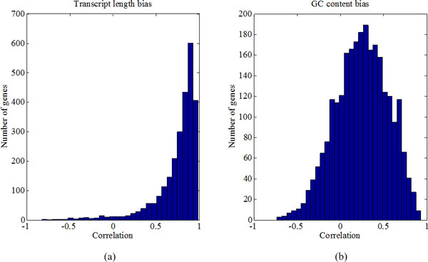
Dissecting read variability into sequencing bias.(a) Estimated over-dispersion parameter U_g,i,j shows strong correlation with transcript location. (b) GC content bias can also be inferred from U_g,i,j. Top expressed 2631 genes (number-of-exons>10) from one TCGA basal sample are used in this study.

Conclusions

Large variation in RNA-Seq data has become the major obstacle against accurate estimation of gene expression and DEG identification. Much effort has been made to model variation across biological replicates, while limited attention is paid to tackle extensive over-dispersion observed in sequencing counts. For short-read sequencing technologies (e.g., Illumina), multiple sources of systematic bias have been identified, including transcript length bias, GC-content bias, etc. However, in-depth investigation of real RNA-Seq datasets has revealed the following complications: 1) Sequencing bias not only changes from one gene to another, but also varies among samples (Figure 2(c) and (d)); 2) Gene expression is jointly influenced by multiple bias factors, which leads to large variation across the entire transcriptome (Figure 6). However, current research activities have been focused on addressing individual bias corrections, which lacks a unified effort to account for total variability in RNA-Seq data. Therefore, we propose the BADGE method to extensively model both within-sample variability (bias and random variance) and between-sample variability (biological variations among replicates or within the same phenotype group) to improve quality of inference.

Competing interests

The authors declare that they have no competing interests.

Declarations

The publication costs for this article were funded by National Institutes of Health (NIH) [CA149653].

Authors' contributions

JG and JX designed and implemented the algorithm. JG, XW, JX designed and performed the computational experiments. JG and JX contributed to the writing. LHC and RC provided their biological guidance on the breast cancer study. All authors read and approved the final manuscript.

Supplementary Material

Additional file 1

Supplementary materials. This additional file contains supplementary information for the main text, including parameter setting for BADGE method, computational implementation, simulation design, supplementary figures and tables, etc.

Acknowledgements

This work is supported by National Institutes of Health (NIH) [CA149653, CA149147, CA164384, and NS29525-18A, in part].

This article has been published as part of BMC Bioinformatics Volume 15 Supplement 9, 2014: Proceedings of the Fourth Annual RECOMB Satellite Workshop on Massively Parallel Sequencing (RECOMB-Seq 2014). The full contents of the supplement are available online at http://www.biomedcentral.com/bmcbioinformatics/supplements/15/S9.

References

- Trapnell C, Williams BA, Pertea G, Mortazavi A, Kwan G, van Baren MJ, Salzberg SL, Wold BJ, Pachter L. Transcript assembly and quantification by RNA-Seq reveals unannotated transcripts and isoform switching during cell differentiation. Nat Biotechnol. 2010;28(5):511–515. doi: 10.1038/nbt.1621. [DOI] [PMC free article] [PubMed] [Google Scholar]
- Li W, Feng J, Jiang T. IsoLasso: a LASSO regression approach to RNA-Seq based transcriptome assembly. J Comput Biol. 2011;18(11):1693–1707. doi: 10.1089/cmb.2011.0171. [DOI] [PMC free article] [PubMed] [Google Scholar]
- Li JJ, Jiang CR, Brown JB, Huang H, Bickel PJ. Sparse linear modeling of next-generation mRNA sequencing (RNA-Seq) data for isoform discovery and abundance estimation. Proc Natl Acad Sci USA. 2011;108(50):19867–19872. doi: 10.1073/pnas.1113972108. [DOI] [PMC free article] [PubMed] [Google Scholar]
- Zheng S, Chen L. A hierarchical Bayesian model for comparing transcriptomes at the individual transcript isoform level. Nucleic Acids Res. 2009;37(10):e75. doi: 10.1093/nar/gkp282. [DOI] [PMC free article] [PubMed] [Google Scholar]
- Wu Z, Wang X, Zhang X. Using non-uniform read distribution models to improve isoform expression inference in RNA-Seq. Bioinformatics. 2011;27(4):502–508. doi: 10.1093/bioinformatics/btq696. [DOI] [PubMed] [Google Scholar]
- Hansen KD, Irizarry RA, Wu Z. Removing technical variability in RNA-seq data using conditional quantile normalization. Biostatistics. 2012;13(2):204–216. doi: 10.1093/biostatistics/kxr054. [DOI] [PMC free article] [PubMed] [Google Scholar]
- Hansen KD, Brenner SE, Dudoit S. Biases in Illumina transcriptome sequencing caused by random hexamer priming. Nucleic Acids Res. 2010;38(12):e131. doi: 10.1093/nar/gkq224. [DOI] [PMC free article] [PubMed] [Google Scholar]
- Robinson MD, McCarthy DJ, Smyth GK. edgeR: a Bioconductor package for differential expression analysis of digital gene expression data. Bioinformatics. 2010;26(1):139–140. doi: 10.1093/bioinformatics/btp616. [DOI] [PMC free article] [PubMed] [Google Scholar]
- Anders S, Huber W. Differential expression analysis for sequence count data. Genome Biol. 2010;11(10):R106. doi: 10.1186/gb-2010-11-10-r106. [DOI] [PMC free article] [PubMed] [Google Scholar]
- Wu H, Wang C, Wu Z. A new shrinkage estimator for dispersion improves differential expression detection in RNA-seq data. Biostatistics. 2013;14(2):232–243. doi: 10.1093/biostatistics/kxs033. [DOI] [PMC free article] [PubMed] [Google Scholar]
- Leng N, Dawson JA, Thomson JA, Ruotti V, Rissman AI, Smits BM, Haag JD, Gould MN, Stewart RM, Kendziorski C. EBSeq: an empirical Bayes hierarchical model for inference in RNA-seq experiments. Bioinformatics. 2013;29(8):1035–1043. doi: 10.1093/bioinformatics/btt087. [DOI] [PMC free article] [PubMed] [Google Scholar]
- Trapnell C, Hendrickson DG, Sauvageau M, Goff L, Rinn JL, Pachter L. Differential analysis of gene regulation at transcript resolution with RNA-seq. Nat Biotechnol. 2013;31(1):46–53. doi: 10.1038/nbt.2450. [DOI] [PMC free article] [PubMed] [Google Scholar]
- Hu M, Zhu Y, Taylor JM, Liu JS, Qin ZS. Using Poisson mixed-effects model to quantify transcript-level gene expression in RNA-Seq. Bioinformatics. 2012;28(1):63–68. doi: 10.1093/bioinformatics/btr616. [DOI] [PMC free article] [PubMed] [Google Scholar]
- Wei Z, Li H. A Markov random field model for network-based analysis of genomic data. Bioinformatics. 2007;23(12):1537–1544. doi: 10.1093/bioinformatics/btm129. [DOI] [PubMed] [Google Scholar]
- Lawrence CE, Altschul SF, Boguski MS, Liu JS, Neuwald AF, Wootton JC. Detecting subtle sequence signals: a Gibbs sampling strategy for multiple alignment. Science. 1993;262(5131):208–214. doi: 10.1126/science.8211139. [DOI] [PubMed] [Google Scholar]
- Sabatti C, James GM. Bayesian sparse hidden components analysis for transcription regulation networks. Bioinformatics. 2006;22(6):739–746. doi: 10.1093/bioinformatics/btk017. [DOI] [PubMed] [Google Scholar]
- Wang Z, Gerstein M, Snyder M. RNA-Seq: a revolutionary tool for transcriptomics. Nat Rev Genet. 2009;10(1):57–63. doi: 10.1038/nrg2484. [DOI] [PMC free article] [PubMed] [Google Scholar]
- Comprehensive molecular portraits of human breast tumours. Nature. 2012;490(7418):61–70. doi: 10.1038/nature11412. [DOI] [PMC free article] [PubMed] [Google Scholar]
- Cheung VG, Nayak RR, Wang IX, Elwyn S, Cousins SM, Morley M, Spielman RS. Polymorphic cis- and trans-regulation of human gene expression. PLoS Biol. 2010;8(9) doi: 10.1371/journal.pbio.1000480. [DOI] [PMC free article] [PubMed] [Google Scholar]
- Bottomly D, Walter NA, Hunter JE, Darakjian P, Kawane S, Buck KJ, Searles RP, Mooney M, McWeeney SK, Hitzemann R. Evaluating gene expression in C57BL/6J and DBA/2J mouse striatum using RNA-Seq and microarrays. PLoS One. 2011;6(3):e17820. doi: 10.1371/journal.pone.0017820. [DOI] [PMC free article] [PubMed] [Google Scholar]
- Edgren H, Murumagi A, Kangaspeska S, Nicorici D, Hongisto V, Kleivi K, Rye IH, Nyberg S, Wolf M, Borresen-Dale AL. et al. Identification of fusion genes in breast cancer by paired-end RNA-sequencing. Genome Biol. 2011;12(1):R6. doi: 10.1186/gb-2011-12-1-r6. [DOI] [PMC free article] [PubMed] [Google Scholar]
- Mortazavi A, Williams BA, McCue K, Schaeffer L, Wold B. Mapping and quantifying mammalian transcriptomes by RNA-Seq. Nat Methods. 2008;5(7):621–628. doi: 10.1038/nmeth.1226. [DOI] [PubMed] [Google Scholar]
- Tarazona S, Furio-Tari P, Ferrer A, Conesa A. NOISeq: Exploratory analysis and differential expression for RNA-seq data. R package version 200. 2012.
- Dillies MA, Rau A, Aubert J, Hennequet-Antier C, Jeanmougin M, Servant N, Keime C, Marot G, Castel D, Estelle J. et al. A comprehensive evaluation of normalization methods for Illumina high-throughput RNA sequencing data analysis. Brief Bioinform. 2013;14(6):671–683. doi: 10.1093/bib/bbs046. [DOI] [PubMed] [Google Scholar]
- Rapaport F, Khanin R, Liang Y, Pirun M, Krek A, Zumbo P, Mason CE, Socci ND, Betel D. Comprehensive evaluation of differential gene expression analysis methods for RNA-seq data. Genome Biol. 2013;14(9):R95. doi: 10.1186/gb-2013-14-9-r95. [DOI] [PMC free article] [PubMed] [Google Scholar]
- Benjamini Y, Speed TP. Summarizing and correcting the GC content bias in high-throughput sequencing. Nucleic Acids Res. 2012;40(10):e72. doi: 10.1093/nar/gks001. [DOI] [PMC free article] [PubMed] [Google Scholar]
Associated Data
This section collects any data citations, data availability statements, or supplementary materials included in this article.
Supplementary Materials