Diffuse interface models of locally inextensible vesicles in a viscous fluid

Abstract

We present a new diffuse interface model for the dynamics of inextensible vesicles in a viscous fluid with inertial forces. A new feature of this work is the implementation of the local inextensibility condition in the diffuse interface context. Local inextensibility is enforced by using a local Lagrange multiplier, which provides the necessary tension force at the interface. We introduce a new equation for the local Lagrange multiplier whose solution essentially provides a harmonic extension of the multiplier off the interface while maintaining the local inextensibility constraint near the interface. We also develop a local relaxation scheme that dynamically corrects local stretching/compression errors thereby preventing their accumulation. Asymptotic analysis is presented that shows that our new system converges to a relaxed version of the inextensible sharp interface model. This is also verified numerically. To solve the equations, we use an adaptive finite element method with implicit coupling between the Navier-Stokes and the diffuse interface inextensibility equations. Numerical simulations of a single vesicle in a shear flow at different Reynolds numbers demonstrate that errors in enforcing local inextensibility may accumulate and lead to large differences in the dynamics in the tumbling regime and smaller differences in the inclination angle of vesicles in the tank-treading regime. The local relaxation algorithm is shown to prevent the accumulation of stretching and compression errors very effectively. Simulations of two vesicles in an extensional flow show that local inextensibility plays an important role when vesicles are in close proximity by inhibiting fluid drainage in the near contact region.

1. Introduction

Vesicles are fluid-filled sacs bounded by a closed lipid bilayer membrane. Vesicles play a critical role in intracellular transport of molecules and proteins [4]. Vesicles have been used as drug delivery vehicles [56], microreactors [21] and as models of more complex biostructures such as red blood cells (RBCs) [55]. RBCs and vesicles are known to undergo complex motions and shape changes under applied flows (e.g., see [3, 10, 15, 22, 28, 38, 50]) and transitions from stationary shapes (tank-treading) to trembling to tumbling have been observed as a function of flow conditions and membrane characteristics. RBCs resist shear deformation due to the presence of a membrane cytoskeleton and also resist bending and area dilatation (e.g., see [2, 50, 65]), while the lipid bilayer membranes in vesicles are liquid-like, resist bending and are largely inextensible (e.g., see [39, 55]). In this paper, we focus on the dynamics of homogeneous vesicles, although our results apply more generally to the case in which there may be several lipid components on the membrane that can induce the formation of rafts.

Most experimental results on vesicles are performed in the low Reynolds number regime, see e.g. [15, 28, 42]. Under these conditions inertial effects can be neglected and the Stokes limit considered, which allows the development of small-deformation perturbation theories [13, 29, 36, 45, 46, 47, 64], which all qualitatively predict the experimentally observed tank-treading and tumbling motion. Various numerical approaches have also been considered in the Stokes limit to analyze tank-treading and tumbling, e.g. [6, 7, 8, 24, 30, 31, 33, 48, 51, 57, 60, 61, 66]. Except for [30] in which the vesicle shape was assumed to be a fixed ellipsoid, all other models are of Helfrich type and consider a membrane free energy

$$ℰ={\int }_{\mathrm{\Gamma }}\frac{1}{2}{b}_N{(H-H_0)}^{2}d\mathrm{\Gamma }+{\int }_{\mathrm{\Gamma }}{b}_{G}Kd\mathrm{\Gamma }$$ (1)

with membrane Γ(t), total curvature H, spontaneous curvature H₀, normal bending rigidity b_N, Gaussian bending rigidity b_G and Gaussian curvature K. We focus on the case in which the vesicle is homogeneous and its topology does not change. Then b_N, H₀ and b_G may be assumed to be constant and the Gaussian bending energy only contributes a constant and can therefore be neglected. Lagrange multipliers are used to enforce the inextensibility constraint, which can be considered as a global constraint to enforce a constant area of the membrane, but allowing for local variations, or as a stronger local constraint. The jump condition for the fluid stress tensor S = −pI + νD, where p is the pressure, ν is the viscosity, and D is twice the rate of deformation tensor D = ∇v + (∇v)^T, with velocity v, along the membrane then reads

$${[\mathbf{S}·\mathbf{n}]}_{\mathrm{\Gamma }}=\frac{\delta ℰ}{\delta \mathrm{\Gamma }}\text{unconstrained},$$ (2)

$${[\mathbf{S}·\mathbf{n}]}_{\mathrm{\Gamma }}=\frac{\delta ℰ}{\delta \mathrm{\Gamma }}+{\lambda }_{\text{global}}H\mathbf{n}\text{global area constraint},$$ (3)

$${[\mathbf{S}·\mathbf{n}]}_{\mathrm{\Gamma }}=\frac{\delta ℰ}{\delta \mathrm{\Gamma }}+{\lambda }_{\text{local}}H\mathbf{n}+{\mathrm{\nabla }}_{\mathrm{\Gamma }}{\lambda }_{\text{local}}\text{local inextensibility constraint},$$ (4)

where [f]_Γ = f_outer − f_inner, n is the normal pointing out of the vesicle, and ∇_Γ is the surface gradient ∇_Γ = P∇, with the projection operator P = I − n ⊗ n. The Lagrange multipliers are functionals of the fluid velocity v and are obtained by requiring

$$\frac{d}{dt}{\int }_{\mathrm{\Gamma }}d\mathrm{\Gamma }={\int }_{\mathrm{\Gamma }}H\mathbf{v}·\mathbf{n}d\mathrm{\Gamma }=0,\text{global area constraint},$$

$${\mathrm{\nabla }}_{\mathrm{\Gamma }}·\mathbf{v}=0,\text{local inextensibility constraint}.$$

We remark that locally inextensible vesicles also conserve the global surface area. The jump condition for the velocity in all cases is

$${[\mathbf{v}]}_{\mathrm{\Gamma }}=0.$$

Due to the linearity of the Stokes problem, efficient algorithms can be derived to solve the coupled fluid-structure flow problem, e.g. [8, 57, 60, 61, 66]. When inertial forces are considered, the development of efficient algorithms remains a significant challenge.

Inertial effects can become important in a variety of biophysical applications. Flowing vesicles/RBCs in larger blood vessels such as arterioles and arteries may experience Reynolds numbers of order unity or higher, especially if the vessels are constricted due to diseases such as thrombosis, e.g. [5, 62]. Large Reynolds numbers may also be found in biomedical devices such as ventricular assist devices, e.g., [23]. Motivated by these applications inertial effects are considered in [16, 32, 34, 41, 43, 54], which found that the classical tumbling behavior of highly viscous vesicles is no longer observed at moderate Reynolds numbers.

The Navier-Stokes equations inside and outside the vesicle read

$$\rho ({\partial }_t\mathbf{v}+\mathbf{v}·\mathrm{\nabla }\mathbf{v})-\mathrm{\nabla }·\mathbf{S}=0$$ (5)

$$\mathrm{\nabla }·\mathbf{v}=0$$ (6)

with density ρ = ρ_1,2 and stress tensor S = S_1,2 = −pI + ν_1,2D. Here, the notation ρ_1,2 means ρ₁ inside and ρ₂ outside the vesicle. The global area constraint, which can be treated explicitly, has been used by [9] within a front tracking method, by [17, 18, 25, 44] within phase field methods, and was also considered in [53] within a level-set approach.

The local inextensibility constraint is more delicate and leads to additional nonlinear coupling in the model. This has been considered within a level set approach in [16, 34, 53, 54], immersed boundary methods [31, 32] and phase field methods [7, 8, 34, 43]. Capsule-like models have also been considered using strain-energy functions that penalize local stretching, e.g. [12, 41].

In [53, 54] the system is rewritten as a single-fluid model by considering the jump conditions for the fluid stress tensor as a body-force term with a delta-function δ_Γ to localize the force at the membrane. An iterative multi-step projection method is used to ensure first the incompressibility of the fluid and second to determine the Lagrange multiplier. However, the projection step to determine the Lagrange multiplier is fully explicit and does not preserve the incompressibility of the fluid. The approach also assumes that the level set function is a signed distance function, and thus requires redistancing. Further, the inextensibility constraint was enforced throughout the computational domain near the interface, which could influence the velocity field in the bulk fluid phases. In [34, 35], a saddle-point approach was used to solve the level-set formulation of the system using adaptive finite elements. An implicit time-stepping algorithm was proposed where the fluid equations and the level-set equations were solved iteratively at each time step. Additional Lagrange multipliers were introduced into the level-set equation to enhance volume and surface area conservation. Indeed, without these additional Lagrange multipliers, the volume and surface area errors increase rapidly leading to inaccuracy of the method. The additional Lagrange multipliers, however, do not introduce additional forces in the fluid, which is questionable physically. A similar approach is used in [16] although they did not use adaptive local refinement and did not consider the additional Lagrange multipliers in the level-set equation. Instead higher order polynomial approximations were used in the finite element method to increase accuracy, which increases the computational cost. In [43], an other approach was used in the level-set context. In particular, a simple elastic force was introduced to penalize local stretching. This method requires a large elasticity coefficient to generate nearly inextensible membranes that can introduce time step restrictions for stability.

In [26, 31, 32], a single-fluid model was also used with a Lagrange multiplier to enforce inextensibility; the scheme was implemented using a penalty immersed boundary method (pIB) in 2D and in axisymmetric flows. In this approach, the interface is represented by two curves one of which moves with the fluid while the other moves elastically under the influence of bending forces. The two curves are linked by stiff springs, which provide the only forces in the fluid. This approach enables the system for the fluid flow and the elastic and bending forces to be decoupled, which is in the same spirit as the method in [53, 54]. In principle, the method should converge to the original inextensible model as the spring stiffness tends to infinity, although this was not demonstrated and numerically large stiffnesses can introduce severe time step restrictions for stability.

Single-fluid models implemented using the phase field method were presented in [7, 8, 43]. In this approach, a Lagrange multiplier was introduced and was assumed to satisfy an advection-reaction equation where the advective time derivative was proportional to the surface divergence of the velocity field. The constant of proportionality was referred to as a tension-like parameter T. To ensure stability, additional diffusion is introduced which smooths out strong local variations in ∇_Γ · v. As shown in the asymptotic analysis in [7], and further discussed in [27], inextensibility in this approach was only fulfilled in the limit T → ∞ where in practice, T ∼ε⁻¹ and ε is proportional to the thickness of the diffuse interface, which is taken to zero in the asymptotics. Thus, for finite ε, the interface is not fully inextensible. The convergence of the method as ε → 0 was not demonstrated numerically.

Each of the methods discussed above has advantages and disadvantages. A common feature is that all the single-fluid methods require various forms of regularization to implement the dynamics and to enforce the inextensibility of the vesicle membrane to some degree. This is true of our new method as well. However, none of the previously developed methods have been shown to converge numerically to inextensible evolution. As we show here, the dynamics of the vesicle can be very sensitive to the accuracy to which the inextensibility condition is modeled. Thus, there is still a need to develop models for which the accuracy of the inextensibility constraint can be explicitly controlled and for which convergence to the sharp interface model can be demonstrated.

Accordingly, in this paper we present a new diffuse interface model for the dynamics of inextensible vesicles in a viscous fluid with inertia. A new feature of this work is the implementation of the local inextensibility condition in the diffuse interface context. As in the other methods described above, local inextensibility is enforced by using a local Lagrange multiplier, which provides the necessary tension force at the interface. However, we introduce a new equation for the local Lagrange multiplier whose solution essentially provides a harmonic extension of the local Lagrange multiplier off the interface while maintaining the local inextensibility constraint near the interface. The degree to which local inextensibility is enforced is controlled by a regularization parameter that scales with the square of the interface thickness. We demonstrate using asymptotic analysis and numerical simulations that inextensible evolution is obtained when the interface thickness tends to zero. To make the method more robust, we also develop a local relaxation scheme that dynamically corrects local stretching/compression errors. The discretized equations are solved in 2D using an adaptive finite element method.

The outline of the paper is as follows. In Sec. 2, the new diffuse interface models are derived. In Sec. 3, a matched asymptotic analysis of the diffuse models is presented. In Sec. 4, the spatiotemporal discretization of the system is discussed. Numerical results are presented in Sec. 5. In Sec. 6, conclusions are given and future work is discussed. Finally, details on the matched asymptotic analysis are given in an Appendix.

2. Phase Field/Diffuse Interface Models

The phase field method, also known as the diffuse interface method, introduces an auxiliary field ϕ that distinguishes the vesicle interior from the exterior. The vesicle boundary is modeled by a narrow, diffuse layer. An equation is posed for the phase field function ϕ, which is nonlinearly coupled to the fluid equations. In the models presented below, space is nondimensionalized using L, a characteristic length scale (e.g., vesicle size), and time is non-dimensionalized using V/L where V is a characteristic velocity scale (e.g., far-field velocity magnitude). The density and viscosity are nondimensionalized using their values in the matrix fluid. Near the interface, ϕ can be approximated by

$$\varphi (t,\mathbf{x}):=tan\mathrm{h}\left(\frac{-r(t,\mathbf{x})}{\sqrt{2}\epsilon }\right)$$ (7)

where ε characterizes the thickness of the diffuse interface and r(t, x) denotes the signed-distance function between x ∈ Ω and its nearest point on Γ(t). Taking r to be negative inside the vesicle, we label the inside with ϕ ≈ 1 and the outside with ϕ ≈ −1. The interface Γ(t) is implicitly defined by the zero level set of ϕ.

Consider a diffuse interface version of the nondimensional Helfrich energy [19]

$$ℰ(\varphi )={\int }_{\mathrm{\Omega }}\frac{1}{2\epsilon }\frac{1}{\text{ReBe}}{(\epsilon \mathrm{\Delta }\varphi -\frac{1}{\epsilon }({\varphi }^2-1)(\varphi +H_0))}^{2}d\mathrm{\Omega }.$$ (8)

where the Reynolds number is Re = ρ₂VL/ν₂, where ρ₂ and ν₂ are the density and viscosity of the matrix fluid (the fluid outside the vesicle). The bending capillary number is $\text{Be}=\frac{4\sqrt{2}}{3}\cdot \frac{v_2{L}^{2}V}{b_N}$, where b_N is the bending stiffness. The scaling factor 4√2/3 arises from the choice of the double-well potential (ϕ² − 1) (ϕ + H₀) contained in Eq. (8) and is chosen to match the sharp interface energy in the thin interface limit. For example, in [19] a formal convergence analysis as ε → 0 is performed to show that the diffuse interface energy in Eq. (8) tends to the nondimensional form of the sharp interface energy in Eq. (1). This approach differs from the treatment in [8] where the diffuse interface version of the Helfrich energy is the extension of the sharp interface energy in Eq. (1) off the interface into the whole domain Ω with the total curvature and normal vector being calculated as H = ∇ · n and n = −∇ϕ/|∇ϕ|, respectively.

2.1. Global surface area constraint: Model A

A thermodynamically consistent phase field approach to model the dynamics of vesicles in a viscous fluid was proposed in [17, 18]. In this approach, spatially constant Lagrange multipliers were introduced to enforce volume and total (global) surface area conservation, and bending forces obtained variationally from the energy in Eq. (8) were included. The resulting nondimensional Navier-Stokes system is

$$\rho ({\partial }_t\mathbf{v}+\mathbf{v}·\mathrm{\nabla }\mathbf{v})+\mathrm{\nabla }p-\frac{1}{\text{Re}}\mathrm{\nabla }·(\nu \mathbf{D})=g\mathrm{\nabla }\varphi -{\lambda }_{\text{global}}f\mathrm{\nabla }\varphi -{\lambda }_{\text{volume}}\mathrm{\nabla }\varphi ,$$ (9)

$$\mathrm{\nabla }·\mathbf{v}=0,$$ (10)

where λ_global = λ_global(t) ∈ ℝ and λ_volume = λ_volume ∈ ℝ are the Lagrange multipliers and the terms on the right hand side of Eq. (9) are the excess forces due to bending, global surface area conservation and volume conservation respectively. Further,

$$g=\frac{1}{\text{ReBe}}(\mathrm{\Delta }{f}_c-\frac{1}{{\epsilon }^2}(3{\varphi }^2+2H_0\varphi -1)f_c),$$ (11)

$$f_c=\epsilon \mathrm{\Delta }\varphi -\frac{1}{\epsilon }({\varphi }^2-1)(\varphi +H_0),$$ (12)

$$f=\epsilon \mathrm{\Delta }\varphi -\frac{1}{\epsilon }({\varphi }^2-1)\varphi .$$ (13)

The evolution of ϕ is given by the dimensionless nonlinear advection-diffusion equation

$${\partial }_t\varphi +\mathbf{v}·\mathrm{\nabla }\varphi =-\eta (g-{\lambda }_{\text{global}}f-{\lambda }_{\text{volume}}),$$ (14)

where η > 0 is a small mobility parameter. The density ratio and viscosity ratio are modeled as ρ = ρ(ϕ) = 0.5(ϕ+ 1)ρ₁/ρ₂ +0.5(1 − ϕ) and ν = ν(ϕ) = 0.5(ϕ + 1)ν₁/ν₂ +0.5(1 − ϕ), respectively (see also [7, 53]). The Lagrange multipliers λ_volume and λ_global follow from the constraints

$$\frac{d}{dt}\nu (\varphi )=\frac{d}{dt}{\int }_{\mathrm{\Omega }}\frac{1}{2}(\varphi +1)d\mathrm{\Omega }=0(\text{volume constraint})$$ (15)

$$\frac{d}{dt}\mathcal{A}(\varphi )=\frac{d}{dt}{\int }_{\mathrm{\Omega }}\frac{\epsilon }{2}|\mathrm{\nabla }\varphi {|}^2+\frac{1}{4\epsilon }{({\varphi }^2-1)}^{2}d\mathrm{\Omega }=0(\text{global area constraint})$$ (16)

Using the evolution equation for ϕ, the system to be solved for λ_volume and λ_global reads

$${\lambda }_{\text{volume}}{\int }_{\mathrm{\Omega }}d\mathrm{\Omega }+{\lambda }_{\text{global}}{\int }_{\mathrm{\Omega }}fd\mathrm{\Omega }={\int }_{\mathrm{\Omega }}gd\mathrm{\Omega },$$ (17)

$${\lambda }_{\text{volume}}{\int }_{\mathrm{\Omega }}fd\mathrm{\Omega }+{\lambda }_{\text{global}}{\int }_{\mathrm{\Omega }}{f}^{2}d\mathrm{\Omega }={\int }_{\mathrm{\Omega }}(\frac{1}{\eta }\mathbf{v}·\mathrm{\nabla }\varphi +g)fd\mathrm{\Omega },$$ (18)

which must be solved together with Eqs. (9), (10) and (14). Because of the accumulation of errors, [20] suggested that additional relaxation terms be added to the equations, which was found to improve accuracy. That is, the terms $\frac{1}{2\tau }({\mathcal{V}}_0-\mathcal{V}(\varphi ))$ and $\frac{1}{2\tau }({\mathcal{A}}_0-\mathcal{A}(\varphi ))$ are added to the right hand sides of Eqs. (17) and (18), respectively, where ₀ and ₀ denote the desired volume and area. The relaxation parameter is the inverse of the time step size τ.

2.2. Local inextensibility constraint: Model B

To enforce the local inextensibility constraint in the phase-field model, we propose a modification of the flow problem in model A. In particular, we introduce spatially varying Lagrange multiplier λ_local, which introduces tension forces along the interface. These tension forces take the form ∇ · (δ_εP λ_local), where P = I − n ⊗ n, with n = −∇ϕ/|∇ϕ|, is the tangential projection operator and δ_ε = 0.5|∇ϕ| is a diffuse interface approximation of the surface delta function.

The nondimensional Navier-Stokes equation thereby becomes

$$\rho ({\partial }_t\mathbf{v}+\mathbf{v}·\mathrm{\nabla }\mathbf{v})+\mathrm{\nabla }p-\frac{1}{\text{Re}}\mathrm{\nabla }·(\nu \mathbf{D})=\mathrm{\nabla }·({\delta }_{\epsilon }\mathbf{P}{\lambda }_{\text{local}})+g\mathrm{\nabla }\varphi -{\lambda }_{\text{global}}f\mathrm{\nabla }\varphi -{\lambda }_{\text{volume}}\mathrm{\nabla }\varphi ,$$ (19)

$$\mathrm{\nabla }·\mathbf{v}=0,$$ (20)

where we have also retained the volume and global surface area Lagrange multipliers, which we found to help improve the accuracy of the method. The inclusion of the volume and global surface area constraints results in a decreased magnitude of λ_local compared to the case where the constraints are not included. The evolution equation for ϕ as well as the system to determine λ_global and λ_volume remain as before.

The inextensibility constraint ∇_Γ · v = P : ∇v = 0 on Γ is extended off Γ into the whole domain Ω, following the diffuse domain approach [37, 52, 58]. The idea is to perform an extension of the equation in order to solve for λ_local in the whole domain, without extending the inextensibility constraint away from the interface. In particular, we take

$$\xi {\epsilon }^2\mathrm{\nabla }·({\varphi }^2\mathrm{\nabla }{\lambda }_{\text{local}})+{\delta }_{\epsilon }\mathbf{P}:\mathrm{\nabla }\mathbf{v}=0,$$ (21)

where ξ > 0 is a parameter independent of ε. Eq. (21) reduces to Δλ_local = 0 away from Γ, since ϕ² ≈ 1 and δ_ε ≈ 0, and becomes P : ∇v = 0 near Γ, where δ_ε is large and ϕ² ≈ 0. Thus, this effectively provides a harmonic extension of λ_local off Γ while maintaining the local inextensibility constraint near Γ. An asymptotic analysis is given in Sec.3, which shows convergence of Eq. (21) as ε → 0 to the original sharp interface inextensibility constraint. We note that the tension force term in the Navier-Stokes equation expands to ∇ · (δ_εPλ_local) = δ_ε(∇_Γλ_local − λ_localHn), which is exactly the body force term used in [6, 7, 8, 34, 53].

Our approach differs from that taken in the phase field method used in [6, 7, 8, 43], where the evolution equation ∂_tλ_local + v · ∇λ_local = βΔλ_local + TP : ∇v was used instead of Eq. (21). In this equation, T is interpreted as a tension-like constant that effectively controls the inextensibility of the membrane and the diffusion is only added for regularization purposes, with a small parameter β > 0. Note that if T → ∞, such as would be the case if T ~ 1/ε, then the inextensibility condition is enforced throughout the whole domain, which is unlike the formulation considered here. Further, unlike the case here, the additional Lagrange multipliers for volume and global area conservation were not considered.

The above choice of the regularization term is further justified by admitting the following energy law. Consider the total energy

$${ℰ}_{\text{tot}}={\int }_{\mathrm{\Omega }}\frac{1}{2\epsilon }\frac{1}{\text{ReBe}}{(\epsilon \mathrm{\Delta }\varphi -\frac{1}{\epsilon }({\varphi }^2-1)(\varphi +H_0))}^2+\frac{1}{2}|\mathbf{v}{|}^{2}d\mathrm{\Omega }.$$

where we have assumed the kinetic energy with constant density, i.e. the density ratio ρ = 1. Note, that thermodynamically consistent diffuse interface models with different densities are still controversial and either involve additional forces in the Navier-Stokes equation [1] or quasi-incompressibility [40]. The time derivative of the above energy is

$${\mathrm{d}}_t{ℰ}_{\text{tot}}={\int }_{\mathrm{\Omega }}g{\partial }_t\varphi +\mathbf{v}·{\partial }_t\mathbf{v}d\mathrm{\Omega }.$$

Plug in the time evolution equations (9),(10) and (14) and use integration by parts to obtain

$${\mathrm{d}}_t{ℰ}_{\text{tot}}={\int }_{\mathrm{\Omega }}-\eta g(g-{\lambda }_{\text{global}}f-{\lambda }_{\text{volume}})-\mathbf{v}·\mathrm{\nabla }\varphi ({\lambda }_{\text{global}}f+{\lambda }_{\text{volume}})-\frac{\nu }{2\text{Re}}\mathbf{D}:\mathbf{D}+\mathbf{v}·\mathrm{\nabla }·({\delta }_{\epsilon }\mathbf{P}{\lambda }_{\text{local}})d\mathrm{\Omega }.$$

This can be rewritten using Eqs. (17) and (18) multiplied by ηλ_volume and ηλ_global, respectively:

$${\mathrm{d}}_t{ℰ}_{\text{tot}}={\int }_{\mathrm{\Omega }}-\eta {(g-{\lambda }_{\text{global}}f-{\lambda }_{\text{volume}})}^2-\frac{\nu }{2\text{Re}}\mathbf{D}:\mathbf{D}+\mathbf{v}·\mathrm{\nabla }·({\delta }_{\epsilon }\mathbf{P}{\lambda }_{\text{local}})d\mathrm{\Omega }.$$

Finally using the regularized inextensibility equation (21) and integration by parts we obtain decreasing energy

$${\mathrm{d}}_t{ℰ}_{\text{tot}}={\int }_{\mathrm{\Omega }}-\eta {(g-{\lambda }_{\text{global}}f-{\lambda }_{\text{volume}})}^2-\frac{\nu }{2\text{Re}}\mathbf{D}:\mathbf{D}-\xi {\epsilon }^2{\varphi }^2|\mathrm{\nabla }{\lambda }_{\text{local}}{|}^{2}d\mathrm{\Omega }.$$

2.3. Local inextensibility constraint with relaxation Model C

As occurs with the global surface area constraint [20], solving Eq. (21) may introduce small errors at each time step due to the regularization term (first term on the left hand side). Such errors may accumulate over time and may lead to spurious local stretching and compression of the membrane. Hence, it would be desirable to have a local mechanism to correct these errors and drive a slightly stretched or compressed surface back to equilibrium. Such relaxation mechanisms were used in sharp interface models of flexible fibers evolving in a Stokes flow [59]. Here, we present a local relaxation mechanism in the diffuse interface context.

We introduce a variable c to measure local stretching of the interface. Taking c to evolve by the surface mass conservation equation:

$${\partial }_{t}c+\mathbf{v}·\mathrm{\nabla }c+c{\mathrm{\nabla }}_{\mathrm{\Gamma }}·\mathbf{v}=0\text{on}\mathrm{\Gamma },$$ (22)

and setting the initial value c(x, 0) = 1, locations where c deviates from 1 represent regions of compression (c > 1) and stretching (c < 1). For numerical purposes we introduce additional diffusion along the interface

$${\partial }_{t}c+\mathbf{v}·\mathrm{\nabla }c+c{\mathrm{\nabla }}_{\mathrm{\Gamma }}·\mathbf{v}=\theta {\mathrm{\Delta }}_{\mathrm{\Gamma }}c\text{on}\mathrm{\Gamma }$$ (23)

with a small parameter θ > 0. Restricting the diffusion to the interface ensures no interference with the bulk.

We use a version of Hooke's law to relax the local changes in interfacial area. In particular, we require that the strength of the relaxation is proportional to the amount of local stretching and compression. Accordingly, we take ∇_Γ · v = ζ(c −1)/c, where ζ > 0 is a constant controlling the strength of the relaxation. As we will see later in the diffuse interface model, a good choice for ζ is the inverse of the time step size. As long as c = 1 the original inextensibility condition ∇_Γ · v = 0 holds.

Within the diffuse domain formulation we replace Eq. (21) by

$$\xi {\epsilon }^2\mathrm{\nabla }·({\varphi }^2\mathrm{\nabla }{\lambda }_{\text{local}})+{\delta }_{\epsilon }\mathbf{P}:\mathrm{\nabla }\mathbf{v}=\zeta \frac{c-1}{c}{\delta }_{\epsilon },$$ (24)

where the concentration c satisfies a diffuse interface version of Eq. (23),

$${\partial }_{t}c+\mathbf{v}·\mathrm{\nabla }c+c\mathbf{P}:\mathrm{\nabla }\mathbf{v}=\theta \mathrm{\nabla }·(\mathbf{P}\mathrm{\nabla }c),$$ (25)

e.g., see [52]. The complete model including relaxation consists of solving the Navier-Stokes equation (19), (20) and (24) for v, p and λ_local, the surface conservation equation (25) for c, the phase field equation (14) for ϕ, and Eqs. (17)-(18) for the Lagrange multipliers λ_global and λ_volume.

At first glance, model C appears to be similar to the approach presented in [7, 8, 6]. However here, the evolution equation is for c, which serves only to correct errors in local inextensibility, rather than for λ_local as in [7, 8, 6], which generates a tension force in the fluid.

3. Asymptotic analysis

In this section, we use matched asymptotic expansions to show that Eq. (24) converges as ε → 0 to the relaxed version of the sharp interface inextensibility condition

$$\mathbf{P}:\mathrm{\nabla }\mathbf{v}={\mathrm{\nabla }}_{\mathrm{\Gamma }}·\mathbf{v}=\zeta \frac{c-1}{c}$$ (26)

on the membrane surface Γ(t), and Eq. (25) converges to the corresponding sharp interface Eq. (23). In this approach, we expand the variables in powers of the interface thickness ε in regions close to (inner expansion) and far (outer expansion) from the interface. The two expansions are matched in an intermediate region where both expansions are presumed to be valid (e.g., see [11, 49] for a general description of the procedure). Previous work [17, 18] can be used to show that the Navier-Stokes system in models B and C converge to the sharp interface incompressible Navier-Stokes equations with jump conditions given in Eq. (4).

Outer expansion

Away from Γ(t), which is defined as the zero level-set of ϕ, we assume that all variables have a regular expansion in ε. For example, the local Lagrange multiplier can be written as ${\lambda }_{\text{local}}={\lambda }_{\text{local}}^{(0)}+\epsilon {\lambda }_{\text{local}}^{(1)}+\dots$, and likewise for the other variables. Further, away from Γ, we have ϕ = ±1 to all orders and so ∇ϕ = 0 and P = I to all orders. Define the outer regions to be Ω⁺, the exterior of the vesicle, and Ω⁻ the interior of the vesicle. Accordingly, plugging the expansions into the equations and matching powers of ε, Eq. (24) becomes

$$\mathrm{\Delta }{\lambda }_{\text{local}}^{(i)}=0,\text{for}i=0,1,\dots \text{in}{\mathrm{\Omega }}^{\pm }.$$ (27)

The leading order contribution from Eq. (25) is:

$${\partial }_t{c}^{(0)}+{\mathbf{v}}^{(0)}\mathbf{·}\mathrm{\nabla }{c}^{(0)}=\theta \mathrm{\Delta }{c}^{(0)}\text{in}{\mathrm{\Omega }}^{\pm }.$$ (28)

Inner expansion

Near Γ(t), we introduce a local coordinate system

$$\mathbf{x}(\mathbf{s},z;\epsilon )=\mathit{X}(\mathbf{s};\epsilon )+\epsilon z\mathbf{n}(\mathbf{s};\epsilon ),$$ (29)

where X(s; ε) is a parametrization of the interface, n(s; ε) is the interface normal vector that points out of the vesicle into Ω⁺, z is the stretched variable

$$z=\frac{r(\mathbf{x})}{\epsilon },$$ (30)

and r is the signed distance from the point x to Γ(t), which is taken to be negative inside the vesicle. We then assume that all variables can be written as functions of z and s and that in these coordinates the variables have regular expansions in ε. That is, for the velocity field

$$\widehat{\mathit{\upsilon }}(z,\mathbf{s};\epsilon )\equiv \mathbf{v}(\mathit{x};\epsilon )=\mathbf{v}(\mathit{X}(\mathit{s};\epsilon )+\epsilon z\mathit{n}(\mathit{s};\epsilon );\epsilon ),$$ (31)

and the inner expansion is

$$\widehat{\mathit{\upsilon }}(z,\mathit{s};\epsilon )={\widehat{\mathit{\upsilon }}}^{(0)}(z,\mathit{s})+\epsilon {\widehat{\mathit{\upsilon }}}^{(1)}(z,\mathit{s})+{\epsilon }^2{\widehat{\mathit{\upsilon }}}^{(2)}(z,\mathit{s})+\dots .$$ (32)

The definitions and expansions of ϕ̂, λ̂_local and ĉ are analogous. Note that ϕ̂⁽⁰⁾ (z, s) = tanh (−z/√2), which can be justified using the analysis in [17, 18].

Matching conditions

The inner and outer expansions are matched in a region where both expansions are valid. To obtain the matching conditions, we assume that there is a region of overlap where both the expansions are valid, e.g. where εz = (1). In particular, if we evaluate the outer expansion in the inner coordinates, this must match the limits of the inner solutions away from the interface. This procedure provides boundary conditions for the outer equations. Summarizing the results for the velocity field (the matching conditions for the other fields are analogous) we have [49]

$$\underset{z\to \pm \infty }{lim}{\widehat{\mathit{\upsilon }}}^{(0)}(z,\mathit{s})={\mathbf{v}}^{(0)}(\mathbf{X}(\mathbf{s};0)),$$ (33)

at leading order. At the next order, we obtain

$${\widehat{\mathit{\upsilon }}}^{(1)}(z,\mathit{s})={\mathbf{v}}^{(1)}(\mathbf{X}(\mathbf{s};0))+z\mathit{n}\cdot \mathbf{\nabla }{\mathbf{v}}^{(0)}(\mathbf{X}(\mathbf{s};0))+o(1),$$ (34)

as z→±∞, and so on. The quantities on the right hand sides in Eqs. (33) and (34) are the limits from the interior (Ω⁻) and exterior (Ω⁺) of the vesicle. Here o (1) means that the expressions approach equality when z→ ±∞. That is, o (1) is defined such that if some function f(z) = o (1), then we have lim_{z→ ±∞} f(z) = 0.

Analysis near Γ

In the local coordinate system, the derivatives become

$${\partial }_t=-\frac{V}{\epsilon }{\partial }_z+{\partial }_t,$$ (35)

$$\mathbf{\nabla }=\frac{1}{\epsilon }\mathit{n}{\partial }_z+{\mathbf{\nabla }}_{\mathrm{\Gamma }},$$ (36)

$$\mathbf{\Delta }=\frac{1}{{\epsilon }^2}{\partial }_{zz}+\frac{H}{\epsilon }{\partial }_z+{\mathbf{\Delta }}_{\mathrm{\Gamma }},$$ (37)

where V is the normal velocity of Γ. Note that in Eq. (35) we have abused notation; what we mean here is ${\partial }_{t}c=-\frac{V}{\epsilon }{\partial }_z\widehat{c}+{\partial }_t\widehat{c}$ and analogously for the other variables (e.g., see [11, 49]).

Define = P : ∇υ. It can be shown that the inner expansion of this term takes the form

$$\widehat{\mathcal{P}}={\widehat{\mathcal{P}}}^{(0)}+\epsilon {\widehat{\mathcal{P}}}^{(1)}+\dots ,$$ (38)

where the leading term is given by

$${\widehat{\mathcal{P}}}^{(0)}={\mathbf{\nabla }}_{\mathrm{\Gamma }}·{\widehat{\mathit{\upsilon }}}^{(0)}.$$ (39)

Eqs. (38) and (39) are justified in the Appendix. It is also shown in the Appendix that the leading order velocity field fulfills

$${\partial }_z{\widehat{\mathit{\upsilon }}}^{(0)}=\mathbf{0}.$$ (40)

Using this, together with the matching condition (33) we conclude that the outer velocity v⁽⁰⁾ is continuous across the interface. Further, a straightforward calculation shows that

$${\widehat{\delta }}_{\epsilon }=-\frac{1}{2\epsilon }{\widehat{\varphi }}_z^{(0)}+{\widehat{\delta }}_{\epsilon }^{(0)}+\epsilon {\widehat{\delta }}_{\epsilon }^{(1)},$$ (41)

where ${\widehat{\varphi }}_z^{(0)}:={\partial }_z{\widehat{\varphi }}^{(0)}$ and we do not present the specific forms of the higher order terms.

At leading order O(1/ε), Eq. (24) becomes:

$${\widehat{\varphi }}_z^{(0)}{\widehat{\mathcal{P}}}^{(0)}=\zeta \frac{{\widehat{c}}^{(0)}-1}{{\widehat{c}}^{(0)}}{\widehat{\varphi }}_z^{(0)}.$$ (42)

Since ϕ_z < 0, we conclude that ${\widehat{\mathcal{P}}}^{(0)}={\mathbf{\nabla }}_{\mathrm{\Gamma }}·{\widehat{\mathit{\upsilon }}}^{(0)}=\zeta \frac{{\widehat{c}}^{(0)}-1}{{\widehat{c}}^{(0)}}$. Taking the limit as z → ±∞, using the matching condition and the continuity of the velocity, we obtain the inextensibility condition

$${\mathbf{\nabla }}_{\mathrm{\Gamma }}·{\mathbf{v}}^{(0)}=\zeta \frac{c^{(0)}-1}{c^{(0)}}\text{on}\mathrm{\Gamma }(\mathrm{t}),$$ (43)

as claimed.

To analyze Eq. (25) in the inner variables, we use the fact that ${\widehat{\mathit{\upsilon }}}_z^{(0)}=0$ and that the interface moves with the fluid velocity at leading order: V =υ̂⁽⁰⁾ · n. See also [17, 18]. Then, Eq. (25) becomes

$${\partial }_t{\widehat{c}}^{(0)}+{\widehat{\mathit{\upsilon }}}^{(0)}·{\mathrm{\nabla }}_{\mathrm{\Gamma }}{\widehat{c}}^{(0)}+{\widehat{c}}^{(0)}{\mathrm{\nabla }}_{\mathrm{\Gamma }}·{\widehat{\mathit{\upsilon }}}^{(0)}=\theta {\mathrm{\Delta }}_{\mathrm{\Gamma }}{\widehat{c}}^{(0)}.$$ (44)

Taking the limit z → ±∞ and using the leading order matching condition (33) we obtain

$${\partial }_t{c}^{(0)}+{\mathbf{v}}^{(0)}·{\mathrm{\nabla }}_{\mathrm{\Gamma }}{c}^{(0)}+c^{(0)}{\mathrm{\nabla }}_{\mathrm{\Gamma }}·{\mathbf{v}}^{(0)}=\theta {\mathrm{\Delta }}_{\mathrm{\Gamma }}{c}^{(0)},$$ (45)

the solution of which provides the boundary condition for Eq. (28).

4. Numerical methods

To solve the system of equations numerically we split the time interval I = [0, T] into equidistant time intervals 0 = t₀ < t₁ < … and define the time steps τ := t_n+1 − t_n. Of course, adaptive time steps may also be used. We define the discrete time derivative d_t · ⁿ⁺¹ := (· ⁿ⁺¹ − ·ⁿ)/τ, where the upper index denotes the time step number.

The numerical approach for each subproblem is adapted from existing algorithms for the Navier-Stokes equations and the Helfrich model. We solve the overall system using an operator splitting approach, with the Navier-Stokes equations being implicitly coupled to the inextensibility constraint. The phase field variable is solved separately, as are the global Lagrange multipliers and the relaxation variable c.

We present here the time discretization of the inextensibility model with relaxation (model C). At each time step we solve

1. The flow problem for vⁿ⁺¹, pⁿ⁺¹ and ${\lambda }_{\text{local}}^{n+1}$:

   $${\rho }^n(d_t{\mathbf{v}}^{n+1}+{\mathbf{v}}^n·\mathrm{\nabla }{\mathbf{v}}^{n+1})+\mathrm{\nabla }{p}^{n+1}-\frac{1}{\text{Re}}\mathrm{\nabla }·({\nu }^n{\mathbf{D}}^{n+1})-\mathrm{\nabla }·({\delta }_{\epsilon }^n{\mathbf{P}}^n{\lambda }_{\text{local}}^{n+1})=g^n\mathrm{\nabla }{\varphi }^n-{\lambda }_{\text{global}}^n{f}^n\mathrm{\nabla }{\varphi }^n-{\lambda }_{\text{volume}}^n\mathrm{\nabla }{\varphi }^n,$$ (46)

   $$\mathrm{\nabla }·{\mathbf{v}}^{n+1}=0,$$ (47)

   $$\xi {\epsilon }^2\mathrm{\nabla }·({({\varphi }^n)}^2\mathrm{\nabla }{\lambda }_{\text{local}}^{n+1})+{\delta }_{\epsilon }^n{\mathbf{P}}^n:\mathrm{\nabla }{\mathbf{v}}^{n+1}={\tau }^{-1}\frac{c^n-1}{c^n}{\delta }_{\epsilon }^n,$$ (48)

   Where ρⁿ = ρ (ϕⁿ), νⁿ = ν (ϕⁿ), ${\mathbf{P}}^n=\mathbf{I}-\frac{\mathrm{\nabla }{\varphi }^n\otimes \mathrm{\nabla }{\varphi }^n}{|\mathrm{\nabla }{\varphi }^n{|}^2}$ and ${\delta }_{\epsilon }^n=0.5|\mathrm{\nabla }{\varphi }^n|$.

2. The evolution equations for ϕⁿ⁺¹, gⁿ⁺¹, $f_c^{n+1}$ and fⁿ⁺¹:

   $$d_t{\varphi }^{n+1}+{\mathbf{v}}^{n+1}·\mathrm{\nabla }{\varphi }^{n+1}=-\eta (g^{n+1}-{\lambda }_{\text{global}}^n{f}^{n+1}-{\lambda }_{\text{volume}}^n),$$ (49)

   $$g^{n+1}=\frac{1}{\text{ReBe}}(\mathrm{\Delta }{f}_c^{n+1}-\frac{1}{{\epsilon }^2}(3{({\varphi }^{n+1})}^2+2H_0{\varphi }^{n+1}-1)f_c^{n+1}),$$ (50)

   $$f_c^{n+1}=\epsilon \mathrm{\Delta }{\varphi }^{n+1}-\frac{1}{\epsilon }({({\varphi }^{n+1})}^2-1)({\varphi }^{n+1}+H_0),$$ (51)

   $$f^{n+1}=\epsilon \mathrm{\Delta }{\varphi }^{n+1}-\frac{1}{\epsilon }({({\varphi }^{n+1})}^2-1){\varphi }^{n+1}.$$ (52)

   We further linearize the nonlinear terms using a Taylor series expansion of order one, e.g. ((ϕⁿ⁺¹)²− 1)ϕⁿ⁺¹ = ((ϕⁿ)² −1)ϕⁿ+(3(ϕⁿ)²−1)(ϕⁿ⁺¹− ϕⁿ).

3. The equations for the Lagrange multipliers ${\lambda }_{\text{volume}}^{n+1}$ and ${\lambda }_{\text{global}}^{n+1}$:

   $$\begin{array}{c}{\lambda }_{\text{volume}}^{n+1}{\int }_{\mathrm{\Omega }}d\mathrm{\Omega }+{\lambda }_{\text{gobal}}^{n+1}{\int }_{\mathrm{\Omega }}{f}^{n+1}d\mathrm{\Omega }={\int }_{\mathrm{\Omega }}{g}^{n+1}d\mathrm{\Omega }+\frac{1}{2\tau }({\mathcal{V}}_0-\mathcal{V}({\varphi }^{n+1})),\\ {\lambda }_{\text{volume}}^{n+1}{\int }_{\mathrm{\Omega }}{f}^{n+1}d\mathrm{\Omega }+{\lambda }_{\text{global}}^{n+1}{\int }_{\mathrm{\Omega }}{\left(f^{n+1}\right)}^{2}d\mathrm{\Omega }\\ ={\int }_{\mathrm{\Omega }}(\frac{1}{\eta }{\mathbf{v}}^{n+1}·\mathrm{\nabla }{\varphi }^{n+1}+g^{n+1})f^{n+1}d\mathrm{\Omega }+\frac{1}{2\tau }({\mathcal{A}}_0-\mathcal{A}({\varphi }^{n+1})).\end{array}$$

   This system is solvable since the determinant of coefficients on the left hand side is positive, as long as fⁿ⁺¹ is not a constant function.

4. The advection-diffusion equation for the stretching variable cⁿ⁺¹:

   $${\partial }_t{c}^{n+1}+{\mathbf{v}}^{n+1}·\mathrm{\nabla }{c}^{n+1}+c^{n+1}{\mathbf{P}}^{n+1}:\mathrm{\nabla }{\mathbf{v}}^{n+1}=\theta \mathrm{\nabla }·({\mathbf{P}}^{n+1}\mathrm{\nabla }{c}^{n+1}).$$ (53)

To solve the system without relaxation (model B), we omit the right hand side in Eq. 48. For the global area constraint (model A), we additionally omit the last equation of the flow problem in step 1 and set ${\lambda }_{\text{local}}^{n+1}=0$.

We use the adaptive finite element toolbox AMDiS [63] for discretization in space, with the P2/P1 Taylor-Hood element for the flow problem, extended by a P2 element for λ_local. For ϕ and c, P2 elements are used. The resulting linear systems of equations are solved with UMFPACK [14]. The adaptive mesh refinement and coarsening are controlled by the phase field variable, for which a specified spatial resolution at the interface that depends on ε is required. The choices for the numerical parameters η, ξ, ζ and θ are described in the next section.

5. Numerical results

We perform numerical simulations to test models A, B, and C in 2D. We discuss choices of the model parameters and quantify the amount of interface stretching as a function of the interface thickness ε, using two measures of interface stretching. We compare the results using the different models to determine the effect of the corresponding approaches for enforcing the inextensibility condition on the vesicle dynamics. We demonstrate convergence to inextensible evolution as ε → 0. We also investigate the effect of inertia by varying the Reynolds number. We begin using a single vesicle in shear flow and we then simulate two vesicles driven together by an extensional flow. Although the models and numerical methods presented here can be extended to simulate vesicle dynamics in 3D, we defer such simulations to a future work.

Regularization and relaxation parameters

In practice, we find that the regularization coefficient ξ in Eqs. (21) and (24) in models B and C influences the accuracy of the extensibility condition. In particular, increasing ξ leads to larger errors in the enforcement of the inextensibility condition while making ξ small tends to increase the region of inextensibility around the membrane. We find that a good compromise that maintains accuracy while keeping a narrow region of inextensibility is obtained by taking ξ = 1. Note that in Eqs. (21) and (24), ξ is multiplied by ε² so that the overall coefficient of the regularizing term is small and decreases quadratically with ε. Practical considerations also dictate our choice of the relaxation constant ζ from Eq. (24) in model C. As ζ increases, the relaxation occurs more rapidly and leads to small time step restrictions for stability. As ζ decreases, the relaxation occurs more slowly and errors in inextensibility accumulate more readily. We find that a good compromise that maintains accuracy and stability is to take ζ = 1/τ. With this choice, errors in inextensibility from the previous time step are approximately eliminated in the next time step. Finally, for the surface diffusion coefficient θ from Eq. (25) in model C, analogous tradeoffs between accuracy (small θ) and stability (large θ) lead us to choose the compromise value θ = ε/3.

Measurement of inextensibility

There are at least two ways of measuring the inextensibility of the vesicle interface. One can either measure ∇_Γ · v at the interface or one can use the concentration variable c. In the latter case, the value of (c − 1)/c at the interface represents the local stretching accumulated over time while the former case measures the instantaneous stretching. Hence, to test the accuracy of our method we introduce the following two measures of interface stretching:

$$E_{\mathbf{v}}={\int }_{\mathrm{\Omega }}{\epsilon }^{-1}{(1-{\varphi }^2)}^2|{\mathrm{\nabla }}_{\mathrm{\Gamma }}·\mathbf{v}|d\mathrm{\Omega }(\text{instantaneous stretching}),$$ (54)

$$E_c={\int }_{\mathrm{\Omega }}{\epsilon }^{-1}{(1-{\varphi }^2)}^2|(c-1)/c|d\mathrm{\Omega }(\text{accumulated stretching}).$$ (55)

Note that ε⁻¹(1 −ϕ²)² is a (scaled) diffuse interface approximation of the surface delta function.

5.1. Vesicle in shear flow

We simulate a single elliptical vesicle oriented in the y-direction, with major axis of length 2.5 and minor axis of length 1.0, placed in the center of a domain Ω = [0, 4]². We prescribe v = (±10, 0) at the upper/lower boundaries of Ω. Stress-free boundary conditions are imposed for the fluid flow in the x-direction. We use homogeneous Neumann boundary conditions for λ_local, f_c and ϕ, and the Dirichlet boundary condition c = 1. The initial velocity is set to zero. The bending capillary number is taken to be Be = 20, the spontaneous curvature is H₀ = 0, the densities of the fluids inside and outside of the vesicle are matched ρ₁/ρ₂ = 1 and the viscosity ratio is ν₁/ν₂ = 10 so that the viscosity of the fluid inside the vesicle is larger than that of the matrix fluid in the vesicle exterior. To investigate the effect of Reynolds number, we use Re = 1 and Re = 1/200. Finally, the interface thickness is ε = 0.03, the spatial mesh is adaptive with a minimum grid size of h = 2 ⁻⁵ and the time step size τ = 5.0e−4.

5.2. Convergence study and model validation

We first demonstrate that for model B the measure of instantaneous interface stretching E_v converges to zero as ε→ 0. We take Re = 1 and decrease ε, where the grid is refined accordingly to have the same number of grid points across the interface. The results are shown in Fig. 1 at time t = 0.025, which is taken to be small since a fair comparison between the results is only possible if the vesicles are at similar positions. We find that the rate of convergence is between first and second order in ε. Note that results are not shown for models A and C because in both these cases E_v does not converge to zero as ε → 0, albeit for different reasons. In model A, only global stretching is enforced and so there is no control over the amount of local interface stretching. In model C, as indicated by the asymptotic analysis in Sec. 3, the rate of local stretching converges as ε → 0 to ${\mathrm{\nabla }}_{\mathrm{\Gamma }}\cdot \mathbf{v}=\zeta \frac{c-1}{c}$, which is not necessarily equal to 0. For example, if c − 1 = O(τ), then ζ(c − 1) = O(τ) since ζ = 1/τ. This is what we observe in our simulations of model C (results not shown), although as we show next, the relaxation in model C prevents interface stretching from accumulating over time.

Figure 1.

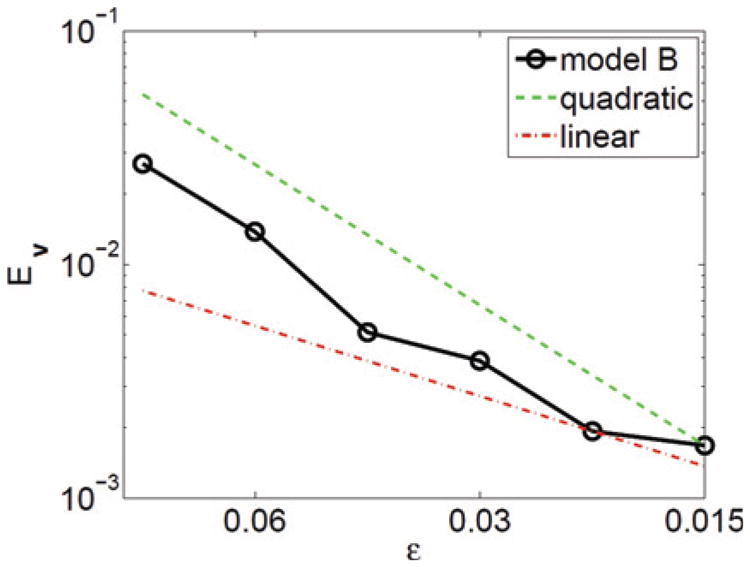
Convergence study showing a super-linear decrease of the instantaneous stretching E_v in Eq. (54) as a function of the interface thickness ε for model B.

In Fig. 2 the accumulated stretching E_c is shown at t = 0.5 for both models B and C. Here, we also find convergence rates between first and second order in both models. Because the simulation time is short, the accumulated stretching is similar in both models, although the accumulated stretching is somewhat smaller in model C as ε is decreased. In Sec. 5.4, we show that at longer times, there are substantial differences in the accumulated stretching between the models.

Figure 2.

Convergence study showing a super-linear decrease of the accumulated stretching E_c in Eq. (55), as a function of the interface thickness ε, for models B (left) and C (right).

The vesicle volume V(ϕ) and the total interface area A(ϕ) are conserved very well for all three models, as seen in Fig. 3. The interface area is slightly better conserved by the use of the local inextensibility constraints in models B and C. The slight drop in interfacial area around t = 0 is due to the fact that the initial interface is not quite equilibrated since the initial interface profile is not represented by a hyperbolic tangent in the normal direction across the interface. Equilibration occurs over the first few time steps. The small variations at early times in the vesicle volume are also due to the equilibration of the interface. The desired reference values for area and volume for the Lagrange multipliers are indicated in Fig. 3 by the dotted black lines and are calculated as the volume and area of the phase field after the first 10 time steps.

Figure 3.

The interfacial area (ϕ) (left), from Eq. (16), and vesicle volume (ϕ) (right), from Eq. (15), for the different models as labeled, with Re = 1. The dotted black line gives the prescribed reference values _o and _o.

5.3. Computational cost of the models

Because models A, B and C require increasing levels of complexity, it is useful to compare the CPU-times for the corresponding algorithms. In Tab. 1, we provide the CPU-time per time step required for each the major subroutines. The CPU-times shown are averaged over the time interval 0 ≤ t ≤ 0.5 using ε = 0.03. The results show that solving the Navier-Stokes equation is the most time consuming part of the simulation. Model A, where there is only a global inextensibility constraint and local inextensibility is not enforced, is the fastest. The additional local inextensibility constraint in models B and C slows down the Navier-Stokes solver by about 30%. In model C the total CPU-time is additionally increased by approximately 4% by solving the equation for c.

Table 1.

The CPU-times for the different models. The values indicate the times (in seconds) for a single solve of the Navier-Stokes equations (46)-(47) with Eq. (48) for models B and C, the Willmore equation (49)-(52) and for model C the advection-diffusion equation for c (53).

	model A	model B	model C
NS (incl. inextensibility)	5.12	6.77	6.83
Willmore	2.01	2.05	2.07
equation for c	-	-	0.32
total	7.13	8.82	9.22

5.4. Vesicle morphologies and comparison of models at longer times

The vesicle morphologies using the different models with ε = 0.03 and Re = 1 and Re = 1/200 are shown in Fig. 4. The red curves correspond to model A, the green to model B and the blue to model C. When Re = 1 (top graphs) the vesicle is in the tank-treading regime and assumes a stationary state around t = 2.0 for all models. At short times (t ≈ 0.5) the local inextensibility constraints in models B and C lead to a faster rotation and thus a smaller inclination angle of the vesicle. This effect is reversed at later times (t ≈ 2.0) where the inclination angle from the stationary vesicle obtained from model A is approximately 0.07 radians smaller than that obtained from models B and C (see Fig. 5 below). Overall, because the vesicle is tank-treading, all the models produce very similar results.

Figure 4.

Time evolution of vesicles in a shear flow with Re = 1 (top) and Re = 1/200 (bottom) using model A (red), model B (green) and model C (blue). The local inextensibility constraints in models B and C tend to slow the rotation of the vesicle, which is particularly noticeable when Re = 1/200.

Figure 5.

The inclination angles (radians) for Re = 1 (left) and Re = 1/200 (right) corresponding to the vesicle dynamics shown in Fig. 4.

When Re = 1/200 (bottom graphs), the vesicle is in the tumbling regime. The vesicle is thus harder to resolve because of the unsteady dynamics. As a result, there are larger differences between the models. The local inextensibility constraints in models B and C significantly delay the time when the vesicle tumbles and decreases the tumbling frequency. This is quantified in Fig. 5 where the inclination angles of the vesicles are shown for the different models with Re = 1 and Re = 1/200.

The accumulated stretching E_c for these simulations is presented in Fig. 6. As expected, the amount of interface stretching rapidly accumulates in model A, is non-monotone in time and saturates when the vesicle tank-treads (Re = 1). When the vesicle tumbles (Re = 1/200), the stretching errors are similarly non-monotone but are larger and appear to accumulate without bound with the most error occurring during the time at which the vesicle rotates rapidly (see the inclination angles in Fig. 5). The local inextensibility constraint in model B suppresses this significantly, but still the stretching accumulates over time. The local relaxation in model C effectively controls the accumulation of stretching. Although a small amount of stretching is observed around t ≈ 5 when the vesicle in model C tumbles, the stretched vesicle interface is rapidly driven back to an unstretched state by the relaxation mechanism. The corresponding spatial distributions of c on the interface Γ(t) are shown at time t = 1 in Fig. 7. The interfaces in models A and B are compressed at the vesicle tips while the sides are stretched. On the other hand, in model C the concentration c ≈ 1 all along the vesicle interface, indicating that there is little overall stretching of the interface. Note that the color scales are different in each case and that the most stretching is observed in model A, as expected.

Figure 6.

The accumulated stretching E_c (55) with Re = 1 (left) and Re = 1/200 (right) corresponding to the vesicle dynamics shown in Fig. 4.

Figure 7.

The value of c along the vesicle interfaces for the different models with Re = 1/200 at time t = 1. Note the different scales indicating minimum and maximum value of c as well as the desired value 1.0. The amount of local stretching/compression decreases from model A to model B to model C.

5.5. Two vesicles in extensional flow

Enforcing local inextensibility becomes more crucial for simulations involving multiple vesicles. To demonstrate this, we use the models to simulate the interactions of two vesicles in an extensional flow and compare the results. A Dirichlet boundary condition is used: v(x, y) = 5(2−x, y−2) at the boundaries of the computational domain Ω = [0, 4]². This corresponds to inflow at the side boundaries and outflow at the upper and lower boundaries. Two elliptical vesicles, oriented in the y-direction, are initially placed at (1,2) and (3,2). The axis lengths are √;2 and 1.0. The remaining parameters are as in Sec. 5.2 with ε = 0.03.

Fig. 8 shows the membranes colored by the values of the surface concentration c and the flow streamlines for the different models. The extensional flow drives the two vesicles to the center of the domain. The results from models B and C are very similar whereas model A predicts behavior that is very different from the other two. At early times (t ≈ 0.005, left column) the streamlines are observed to fan out near the membranes (and vesicle interior) when model A is used, which indicates stretching of the membranes along their sides and compression at their tips. This is even more apparent at later times (middle and right columns) through the values of c. In contrast, the streamlines in models B and C are roughly parallel throughout the vesicles, which indicates that there is little stretching and compression of the membranes. Accordingly, c remains approximately 1 throughout the evolution. At around t = 0.4 the two vesicles in model A meet and finally merge at around t = 0.515. This merging is not seen in the inextensible models, which can be explained as follows. In order for the vesicles to be driven into contact, the fluid in between them has to be squeezed out of the near contact region. When the vesicles are close enough, this process requires a nonzero tangential velocity at the vesicle interfaces. Local inextensibility, however, does not allow such flow, since it would stretch the vesicle interface in the near contact region. Here, this effect is further magnified by the fact that the vesicle interfaces flatten as they approach one another, making it even harder to squeeze the fluid out of the near contact region. Therefore vesicle contact (and coalescence) is inhibited by the local inextensibility in models B and C.

Figure 8.

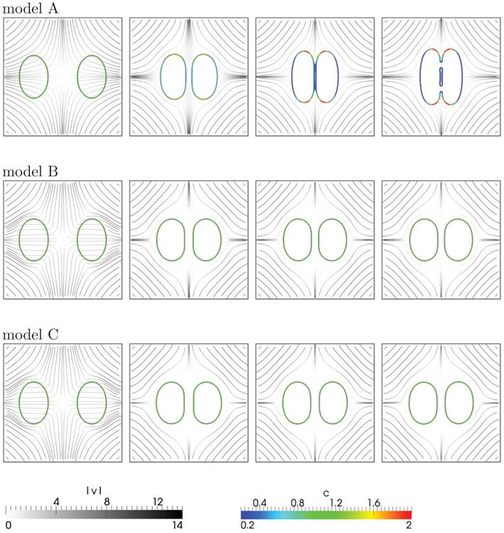
Two vesicles in extensional flow for model A (top row), model B (middle row) and model C (bottom row) at times t = 0.005, 0.18, 0.4, 0.515 (from left to right). The interfaces are colored according to the local values of the surface concentration c. The flow streamlines (grey) are colored by the velocity magnitude |v|. It can be seen that in model A, the interfaces are compressed at the vesicle tips and stretched along the sides. The local inextensibility in models B and C inhibits close contact of the vesicles whereas the local interface stretching in model A enables the vesicles to come into contact and coalesce.

6. Conclusions

We presented a new diffuse interface model for the dynamics of inextensible vesicles in a viscous fluid. Following previous work [6, 7, 8], we used a local Lagrange multiplier to generate a tension force needed to make the vesicle inextensible. However, we introduced a new equation for the local Lagrange multiplier that essentially provides a harmonic extension of the local Lagrange multiplier off the interface while maintaining the local inextensibility constraint near the interface. This is different from the approach taken in [7, 8] where a time-dependent advection-diffusion-reaction equation was used. To make the method more robust we introduced a local relaxation scheme that dynamically corrects stretching/compression errors. In the relaxation scheme, a version of Hooke's law is used where the restoring forces are proportional to the amount of stretching/compression, which is detected by evolving a (surface) concentration field (initialized to one everywhere) and identifying regions where the concentration field deviates from one. Asymptotic analysis demonstrated that our new system converges to a relaxed version of the inextensible sharp interface system.

Compared to the classical sharp interface model for inextensible membranes, our diffuse interface model includes five additional parameters: the interface thickness ε, the mobility η, the regularization ξ, the relaxation rate ζ and the surface diffusion coefficient θ. The first two parameters are present in all diffuse interface models while the latter three parameters are new. We discussed how tradeoffs between accuracy and stability can be used to choose the values of these parameters. Importantly we demonstrated that our new models converge as ε → 0 to inextensible evolution.

To solve the equations numerically we developed an efficient algorithm using an operator splitting approach such that the Navier-Stokes equations were implicitly coupled to the diffuse-interface inextensibility constraint. The phase field equations and the local concentration field were solved separately. Spatial discretization was performed using the adaptive finite element toolbox AMDiS [63] with the P2/P1 Taylor-Hood element being used for the flow problem, extended by a P2 element for the local Lagrange multipliers. P2 elements were also used for the phase field and concentration variables. The resulting nonlinear system was linearized and solved using UMFPACK [14].

We compared the results from our new model with local inextensibility constraints and relaxation (model C) to a model without relaxation (model B) and a previously derived diffuse interface model [17, 18] that conserved only the total surface area (model A). Focusing on the dynamics of a single vesicle in shear flow in 2D, we demonstrated that inextensible evolution is achieved in the sharp interface limit of models B and C. We found that the local inextensibility constraints lead to a larger inclination angle in the tank-treading regime (Re =1). Large differences in the dynamics are observed in the tumbling regime (Re = 1/200) where the local inextensibility constraints in models B and C delay the time at which the vesicle tumbles significantly and increase the length of the tumbling period. The results show that errors in the local inextensibility in models A and B tend to occur during the fast dynamics of tumbling and accumulate over time. The local relaxation in model C prevents this accumulation very effectively. Similar behavior can be observed in sharp interface models (see [59]).

A study of two vesicles driven together by an extensional flow showed a further effect of local inextensibility: the inhibition of close vesicle contact. Fluid drainage out of the near contact region requires tangential forces, which are inhibited by local inextensibility. As a consequence, vesicles were found to remain separated by a finite distance when models B and C were used. But, when model A was used, the vesicles came into close contact and merged precisely because model A does not enforce local inextensibility of the interface.

Future work will use the algorithms presented here to analyze the dependence of the dynamical states of vesicles (tank-treading, tumbling, trembling) on the Reynolds number and other physical parameters (viscosity ratio, density ratio, etc), and the local inextensibility of the interface. We will compare our results with those obtained previously (e.g., [6, 8, 30, 34, 54]). We also plan to extend our algorithms to 3D, replacing the direct UMFPACK solver with a more efficient preconditioned iterative solver for the coupled system, and to incorporate membrane elasticity to provide a more realistic model of red blood cells.

Appendix

Here, we provide justifications for the claims made in Sec. 3. In particular, we show that in the inner variables has a regular expansion in  , where the leading order term is ∇_Γ · v⁽⁰⁾, and that ${\widehat{\mathit{\upsilon }}}_z^{\left(0\right)}:={\partial }_z{\widehat{\mathit{\upsilon }}}^{\left(0\right)}=\mathbf{0}$.

Regular expansion for

Recall that = P:∇v, where P = I − n⊗n is the tangential projection operator. A straightforward calculation shows that

$$\mathcal{P}=\mathrm{\nabla }·(\mathbf{P}\mathbf{v})-(\mathrm{\nabla }·\mathbf{P})·\mathbf{v}$$ (56)

Therefore, in the inner variables, we obtain

$$\begin{array}{c}\widehat{\mathcal{P}}=\frac{1}{\epsilon }\mathbf{n}·(\mathbf{P}{\widehat{\mathit{\upsilon }}}_z)+{\mathrm{\nabla }}_{\mathrm{\Gamma }}·(\mathbf{P}\widehat{\mathit{\upsilon }})-({\mathrm{\nabla }}_{\mathrm{\Gamma }}·\mathbf{P})·\widehat{\mathit{\upsilon }},\\ ={\mathrm{\nabla }}_{\mathrm{\Gamma }}·(\mathbf{P}\widehat{\mathit{\upsilon }})-({\mathrm{\nabla }}_{\mathrm{\Gamma }}·\mathbf{P})·\widehat{\mathit{\upsilon }},\end{array}$$ (57)

since P_z = 0 and n· (Pυ̂_z) = 0. Plugging the inner expansion for υ̂ into Eq. (57) we obtain a regular expansion = ⁽⁰⁾+ε ⁽¹⁾ +… and we recognize the first term as

$${\widehat{\mathcal{P}}}^{(0)}={\mathrm{\nabla }}_{\mathrm{\Gamma }}·(\mathbf{P}{\widehat{\mathit{\upsilon }}}^{(0)})+H{\widehat{\mathit{\upsilon }}}^{(0)}·\mathbf{n}={\mathrm{\nabla }}_{\mathrm{\Gamma }}·{\widehat{\mathit{\upsilon }}}^{(0)}={\mathrm{\nabla }}_{\mathrm{\Gamma }}·{\mathbf{v}}^{(0)}$$ (58)

as claimed (assuming ${\widehat{\mathit{\upsilon }}}_z^{\left(0\right)}=0$).

Behavior of υ̂⁽⁰⁾

Writing the incompressibility condition ∇·v =0 in the inner region, we obtain

$$\frac{1}{\epsilon }{\partial }_z(\widehat{\mathit{\upsilon }}·\mathbf{n})+{\mathrm{\nabla }}_{\mathrm{\Gamma }}·\widehat{\mathit{\upsilon }}=0.$$ (59)

We thus obtain

$${\partial }_z({\widehat{\mathit{\upsilon }}}^{(0)}·\mathbf{n})=0\text{at}\mathrm{O}(1/\epsilon ),$$ (60)

$${\widehat{\mathit{\upsilon }}}_z^{(1)}·\mathbf{n}+{\mathrm{\nabla }}_{\mathrm{\Gamma }}·{\widehat{\mathit{\upsilon }}}^{(0)}=0\text{at}\mathrm{O}(1),$$ (61)

and so on. To complete the claim, we need to show that the tangential components of the velocity, namely Pυ̂⁽⁰⁾, are also independent of z. This follows from the viscous term in the Navier-Stokes equations. It can be shown that this term provides the highest order terms in the inner expansion of the Navier-Stokes equations (see [17, 18]). Thus at the leading order, O(1/ε²), the Navier-Stokes equations become

$${\partial }_z(\nu {\widehat{\mathit{\upsilon }}}_z^{(0)}·\mathbf{n})\mathbf{n}+{\partial }_z(\nu {\partial }_z(\mathbf{P}{\widehat{\mathit{\upsilon }}}^{(0)}))=0.$$ (62)

Since the first term is zero, we conclude that ν∂_z (P υ̂⁽⁰⁾) = constant. Taking z →±∞ and using the leading order matching condition (33), we find that the constant is equal to zero, which proves the claim.

References

- 1.Helmut Abels, Harald Garcke, Günther Grün. Thermodynamically consistent, frame indifferent diffuse interface models for incompressible two-phase flows with different densities. Mathematical Models and Methods in Applied Sciences. 2012;22(03) [Google Scholar]
- 2.Abkarian M, Faivre M, Horton R, Smistrup K, Best-Poescu CA, Stone HA. Cellular-scale hydrodynamics. Biomed Mater. 2008:034011. doi: 10.1088/1748-6041/3/3/034011. [DOI] [PubMed] [Google Scholar]
- 3.Abkarian M, Viallat A. Vesicles and red blood cells in shear flow. Soft Matter. 2008;4:653–657. doi: 10.1039/b716612e. [DOI] [PubMed] [Google Scholar]
- 4.Alberts B, Bray D, Lewis J, Raff M, Robers K, Watson JD. Molecular biology of the cell. Garland: 1994. [Google Scholar]
- 5.Bark DL, Ku DN. Wall shear over high degree stenoses pertinent to atherothrombosis. J Biomech. 2010;43:2970–2977. doi: 10.1016/j.jbiomech.2010.07.011. [DOI] [PubMed] [Google Scholar]
- 6.Beaucourt J, Rioual F, Seon T, Biben T, Misbah C. Steady to unsteady dynamics of a vesicle in a flow. Physical Review E. 2004;69:011906. doi: 10.1103/PhysRevE.69.011906. [DOI] [PubMed] [Google Scholar]
- 7.Biben T, Kassner K, Misbah C. Phase-field approach to three-dimensional vesicle dynamics. Physical Review E. 2005;72:041921. doi: 10.1103/PhysRevE.72.041921. [DOI] [PubMed] [Google Scholar]
- 8.Biben T, Misbah C. Tumbling of vesicles under shear flow within an advected-field approach. Physical Review E. 2003;67:031908. doi: 10.1103/PhysRevE.67.031908. [DOI] [PubMed] [Google Scholar]
- 9.Bonito A, Nochetto RH, Pauletti MS. Dynamics of biomembranes: effect of the bulk fluid. Mathematical Modelling of natural phenomena. 2011;6:25–43. [Google Scholar]
- 10.Brown FLH. Continuum simulations of membrane dynamics and the importance of hydrodynamic effects. Quart Rev Biophys. 2011;44(4):391–432. doi: 10.1017/S0033583511000047. [DOI] [PubMed] [Google Scholar]
- 11.Caginalp G, Fife PC. Dynamics of layered interfaces arising from phase boundaries. SIAM Journal on Applied Mathematics. 1988;48:506–518. [Google Scholar]
- 12.Cordasco D, Bagchi P. Orbital drift of capsules and red blood cells in shear flow. Phys Fluids. 2013;25:091902. [Google Scholar]
- 13.Danker G, Biben T, Podgorski T, Verdier C, Misbah C. Dynamics and rheology of a dilute suspension of vesicles: Higher-order theory. Physical Review E. 2007;76:041905. doi: 10.1103/PhysRevE.76.041905. [DOI] [PubMed] [Google Scholar]
- 14.Timothy A Davis. Algorithm 832: UMFPACK V4.3—an unsymmetric-pattern multifrontal method. ACM Trans Math Softw. 2004 Jun;30(2):196–199. [Google Scholar]
- 15.Deschamps J, Kantsler V, Segre E, Steinberg V. Dynamics of a vesicle in general flow. Proc Nat Acad Sci USA. 2009 Jul;106(28):11444–11447. doi: 10.1073/pnas.0902657106. [DOI] [PMC free article] [PubMed] [Google Scholar]
- 16.Doyeux V, Guyot Y, Chabannes V, Prud'homme C, Ismail M. Simulation of two-fluid flows using a finite element/level set method. application to bubbles and vesicle dynamics. J Comput Appl Math. 2013;246:251–259. [Google Scholar]
- 17.Du Q, Li M, Liu C. Analysis of a phase field Navier-Stokes vesicle-fluid interaction model. Discrete and Continuous Dynamical Systems. 2007;8:539–556. [Google Scholar]
- 18.Du Q, Liu C, Ryham R, Wang X. Energetic variational approaches in modeling vesicle and fluid interactions. Physica D. 2009;238:923–930. [Google Scholar]
- 19.Du Q, Liu C, Ryham R, Wang XQ. A phase field formulation of the Willmore problem. Nonlinearity. 2005;18:1249–1267. [Google Scholar]
- 20.Du Q, Wang XQ. Simulating the deformation of vesicle membranes under elastic bending energy in three dimensions. Journal of Computational Physics. 2006;212:757–777. [Google Scholar]
- 21.Fischer A, Franco A, Oberholzer T. Giant vesicles as microreactors for enzymatic mRNA synthesis. Chembiochem. 2002;3:409–417. doi: 10.1002/1439-7633(20020503)3:5<409::AID-CBIC409>3.0.CO;2-P. [DOI] [PubMed] [Google Scholar]
- 22.Fischer TM, Stohrliesen M, Schmidschonbein H. Red-cell as a fluid particle - tank tread-like motion of human erythocyte-membrane in shear flow. Science. 1978;202:894–896. doi: 10.1126/science.715448. [DOI] [PubMed] [Google Scholar]
- 23.Fraser KH, Taskin ME, Griffith BP, Wu Z. The use of computational fluid dynamics in the development of ventricular assist devices. Med Engng Phys. 2011;33:263–280. doi: 10.1016/j.medengphy.2010.10.014. [DOI] [PMC free article] [PubMed] [Google Scholar]
- 24.Ghigliotti G, Biben T, Misbah C. Rheology of a dilute two-dimensional suspension of vesicles. Journal of Fluid Mechanics. 2010;653:489–518. [Google Scholar]
- 25.Hauβer F, Marth W, Li S, Lowengrub J, Rätz A, Voigt A. Thermodynamically consistent models for two-component vesicles. International Journal of Biomathematics and Biostatistics. 2013;2:19–48. [Google Scholar]
- 26.Hu WF, Kim Y, Lai MC. An immersed boundary method for simulating the dynamics of three-dimensional axisymmetric vesicles in Navier–Stokes flows. J Comput Phys. 2014;257:670–686. [Google Scholar]
- 27.Jamet D, Misbah C. Towards a thermodynamically consistent picture of the phase-field model of vesicles: Local membrane incompressibility. Physical Review E. 2007;76:051907. doi: 10.1103/PhysRevE.76.051907. [DOI] [PubMed] [Google Scholar]
- 28.Kantsler V, Steinberg V. Transition to tumbling and two regimes of tumbling motion of a vesicle in shear flow. Physical Review Letters. 2006;96:036001. doi: 10.1103/PhysRevLett.96.036001. [DOI] [PubMed] [Google Scholar]
- 29.Kaouri B, Farutin A, Misbah C. Vesicles under simple shear flow: Elucidating the role of relevant control parameters. Physical Review E. 2009;80:061905. doi: 10.1103/PhysRevE.80.061905. [DOI] [PubMed] [Google Scholar]
- 30.Keller SR, Skalak R. Motion of a tank-treading ellipsoidal particle in a shear-flow. Journal of Fluid Mechanics. 1982;120:27–47. [Google Scholar]
- 31.Kim Y, Lai MC. Simulating the dynamics of inextensible vesicles by the penalty immersed boundary method. Journal of Computational Physics. 2010;229:4840–4853. [Google Scholar]
- 32.Kim Y, Lai MC. Numerical study of viscosity and inertial effects on tank-treading and tumbling motions of vesicles under shear flow. Phys Rev E. 2012;86:066321. doi: 10.1103/PhysRevE.86.066321. [DOI] [PubMed] [Google Scholar]
- 33.Kraus M, Wintz W, Seifert U, Lipowsky R. Fluid vesicle in shear flow. Physical Review Letters. 1996;77:3685–3688. doi: 10.1103/PhysRevLett.77.3685. [DOI] [PubMed] [Google Scholar]
- 34.Laadhari A, Saramito P, Misbah C. Vesicle tumbling inhibited by inertia. Physica of Fluids. 2012;24:031901. [Google Scholar]
- 35.Laadhari A, Saramito P, Misbah C. Computing the dynamics of biomembranes by combining conservative level set and adaptive finite element methods. CNRS preprint. 2013 URL: http://hal.archives-ouvertes.fr/hal-00604145/en/
- 36.Lebedev VV, Turitsyn KS, Vergeles SS. Dynamics of nearly spherical vesicles in an external flow. Physical Review Letters. 2007;99:218101. doi: 10.1103/PhysRevLett.99.218101. [DOI] [PubMed] [Google Scholar]
- 37.Li X, Lowengrub J, Rätz A, Voigt A. Solving PDEs in complex geometries: A diffuse domain approach. Comm Math Sci. 2009;7:81–107. doi: 10.4310/cms.2009.v7.n1.a4. [DOI] [PMC free article] [PubMed] [Google Scholar]
- 38.Li X, Vlahovska PM, Karniadakis GE. Continuum- and particle-based modeling of shapes and dynamics of red blood cells in health and disease. Soft Matter. 2013;9:28–37. doi: 10.1039/C2SM26891D. [DOI] [PMC free article] [PubMed] [Google Scholar]
- 39.Lipowsky R. The conformation of membranes. Nature. 1991;349:475–481. doi: 10.1038/349475a0. [DOI] [PubMed] [Google Scholar]
- 40.Lowengrub J, Truskinovsky L. Quasi–incompressible cahn–hilliard fluids and topological transitions. Proceedings of the Royal Society of London Series A: Mathematical, Physical and Engineering Sciences. 1998;454(1978):2617–2654. [Google Scholar]
- 41.Luo ZY, Wang SQ, He L, Xu F, Bai BF. Inertia-dependent dynamics of three-dimensional vesicles and red blood cells in shear flow. Soft Matter. 2013;9:9651–9660. doi: 10.1039/c3sm51823j. [DOI] [PubMed] [Google Scholar]
- 42.Mader MA, Vitkova V, Abkarian M, Viallat A, Podgorski T. Dynamics of viscous vesicles in shear flow. European Physics Journal E. 2006;19:389–397. doi: 10.1140/epje/i2005-10058-x. [DOI] [PubMed] [Google Scholar]
- 43.Maitre E, Misbah C, Peyla P, Raoult A. Comparison between advected-field and level-set methods in the study of vesicle dynamics. Physica D. 2012;241:1146–1157. [Google Scholar]
- 44.Marth W, Voigt A. Signaling networks and cell motility: a computational approach using a phase field description. Journal of Mathematical Biology. 2013 doi: 10.1007/s00285-013-0704-4. [DOI] [PubMed] [Google Scholar]
- 45.Messlinger S, Schmidt B, Noguchi H, Gompper G. Dynamic regimes and hydrodynamic lift of viscous vesicles under shear. Physical Review E. 2009;80:011901. doi: 10.1103/PhysRevE.80.011901. [DOI] [PubMed] [Google Scholar]
- 46.Misbah C. Vacillating breathing and tumbling of vesicles under shear flow. Physical Review Letters. 2007;96:028104. doi: 10.1103/PhysRevLett.96.028104. [DOI] [PubMed] [Google Scholar]
- 47.Noguchi H, Gompper G. Swinging and tumbling of a fluid vesicles in shear flow. Physical Review Letters. 2007;98:128103. doi: 10.1103/PhysRevLett.98.128103. [DOI] [PubMed] [Google Scholar]
- 48.Peco C, Rosolen A, Arroyo M. An adaptive meshfree method for phase-field models of biomembranes. part ii: A lagrangian approach for membranes in viscous fluids. J Comput Phys. 2013;249:320–336. [Google Scholar]
- 49.Pego RL. Front migration in the nonlinear Cahn-Hilliard equation. Proceedings of the Royal Society A. 1989;422:261–278. [Google Scholar]
- 50.P M, Barthes-Biesel D, Misbahz C. Flow dynamics of red blood cells and their biomimetic counterparts. C R Physique. 2013;14:451–458. [Google Scholar]
- 51.Rahimian A, Veerapaneni SK, Biros G. Dynamic simulation of locally inextensible vesicles suspended in an arbitrary two-dimensional domain, a boundary integral method. J Comput Phys. 2010;229:6466–6484. [Google Scholar]
- 52.Rätz A, Voigt A. PDE's on surfaces - a diffuse interface approach. Communications in Mathematical Science. 2006;4:575–590. [Google Scholar]
- 53.Salac D, Miksis M. A level set projection model of lipid vesicles in general flows. Journal of Computational Physics. 2011;230:8192–8215. [Google Scholar]
- 54.Salac D, Miksis MJ. Reynolds number effects on lipid vesicles. Journal of Fluid Mechanics. 2012;711:122–146. [Google Scholar]
- 55.Seifert U. Configurations of fluid membranes and vesicles. Adv Phys. 1997;46:13–137. [Google Scholar]
- 56.Sofou S. Surface-active liposomes for targeted cancer therapy. Nanomedicine. 2007;2:711–724. doi: 10.2217/17435889.2.5.711. [DOI] [PubMed] [Google Scholar]
- 57.Sohn JS, Tseng YH, Li S, Voigt A, Lowengrub J. Dynamics of multicomponent vesicles in a viscous fluid. Journal of Computational Physics. 2010;229:119–144. doi: 10.1016/j.jcp.2009.09.017. [DOI] [PMC free article] [PubMed] [Google Scholar]
- 58.Teigen KE, Li X, Lowengrub J, Wang F, Voigt A. A diffuse-interface approach for modeling transport, diffusion and adsorption/desorption of material quantities on a deforming interface. Comm Math Sci. 2009;7:1009–1037. doi: 10.4310/cms.2009.v7.n4.a10. [DOI] [PMC free article] [PubMed] [Google Scholar]
- 59.Tornberg AK, Shelley MJ. Simulating the dynamics and interactions of flexible fibers in stokes flows. J Comput Phys. 2004;196:8–40. [Google Scholar]
- 60.Veerapaneni SK, Gueyffier D, Zorin D, Biros G. A boundary integral method for simulating the dynamics of inextensible vesicles suspended in a viscous fluid in 2d. Journal of Computational Physics. 2009;228:2334–2353. [Google Scholar]
- 61.Veerapaneni SK, Rahimian A, Biros G, Zorin D. A fast algorithm for simulating vesicle flows in three dimensions. J Comput Phys. 2011;230:5610–5634. [Google Scholar]
- 62.Vennemann P, Lindken R, Westerweel J. In vivo whole-field blood velocity measurement techniques. Exp Fluids. 2007;42:495–511. [Google Scholar]
- 63.Vey S, Voigt A. Amdis: adaptive multidimensional simulations. Computing and Visualization in Science. 2007 Mar;10(1):57–67. [Google Scholar]
- 64.Vlahovska PM, Gracia RS. Dynamics of a viscous vesicle in linear flows. Physical Review E. 2007;75:016313. doi: 10.1103/PhysRevE.75.016313. [DOI] [PubMed] [Google Scholar]
- 65.Wan J, Forsyth AM, Stone HA. Red blood cell dynamics: From cell deformation to ATP release. Integr Biol. 2011;3:972–981. doi: 10.1039/c1ib00044f. [DOI] [PubMed] [Google Scholar]
- 66.Zhao H, Shaqfeh ESG. The dynamics of a vesicle in simple shear flow. Journal of Fluid Mechanics. 2011;674:578–604. [Google Scholar]