Parameter Selection in Mutual Information-Based Feature Selection in Automated Diagnosis of Multiple Epilepsies Using Scalp EEG

Abstract

Developing EEG-based computer aided diagnostic (CAD) tools would allow identification of epilepsy in individuals who have experienced possible seizures, yet such an algorithm requires efficient identification of meaningful features out of potentially more than 35,000 features of EEG activity. Mutual information can be used to identify a subset of minimally-redundant and maximally relevant (mRMR) features but requires a priori selection of two parameters: the number of features of interest and the number of quantization levels into which the continuous features are binned. Here we characterize the variance of cross-validation accuracy with respect to changes in these parameters for four classes of machine learning (ML) algorithms. This assesses the efficiency of combining mRMR with each of these algorithms by assessing when the variance of cross-validation accuracy is minimized and demonstrates how naive parameter selection may artificially depress accuracy. Our results can be used to improve the understanding of how feature selection interacts with four classes of ML algorithms and provide guidance for better a priori parameter selection in situations where an overwhelming number of redundant, noisy features are available for classification.

I. Introduction

The accuracy of machine learning (ML) relies on the identification of salient features that reflect, at least partially, the discrimination in question. Ideally that feature space is sparse and, in clinical classification, it is based on biological features with prior likelihood of involvement in the medical condition. In complex, heterogeneous clinical syndromes, such as epilepsy, there are large numbers of computational features with sound biological support. ML methods can be used to identify features that discriminate the patients from controls. This can elucidate the pathology underlying complex disorders but there are an overwhelming number of possible features, many of which are redundant. A key challenge to this approach is: how does one select the number of features to include?

ML methods often use a hypothesis-driven approach to select a small subset of features and explain their discriminative efficacy without reference to excluded features. The salience of these hypothesized features can be confirmed using principled data-driven feature selection algorithms that leverage features against each other and results in a better characterization and therefore classification of disease. Mutual information (MI) is particularly capable of considering the interactions of thousands of features simultaneously, using model-free methods to identify those that are minimally-redundant and maximally-relevant (mRMR) to the classification [1]. This depends on the choice of two parameters: the number of quantal levels, Q, in which to bin the continuous features, and the number of features, F, selected to classify.

In this work we use resting state EEG data to distinguish whether a given patient suffers from epilepsy or instead has experienced non-epileptic seizures (NES). Conventional methods initially miss greater than 50% of patients with epilepsy and further assessment inadequately diagnoses up to 30% of patients. Starting from roughly 40,000 different summaries (features) per subject of EEG behavior, we use mRMR to select features and create an ML classifier that discriminates between epilepsy and NES. We demonstrate how parameter choices of (Q,F) affect the mean and variability of the cross-validation accuracy; arbitrary parameter selection can lead to models that systematically classify worse than chance while naïve attempts to optimize parameters within the model can lead to bias. We demonstrate the varying effect of parameter selection on four classes of machine learning algorithms: Support Vector Machines (SVM), Multilayer Perceptrons (MLP), Bayesian Logistic Regression (BLR) and Alternative Decision Trees (ADT). Accurate discrimination will translate directly to reduced morbidity, and the results of our sampling of the parameter space can be used to guide others in the selection of these critical parameters when utilizing mRMR.

In mRMR, all continuous features must be smoothed into Q a priori selected discrete bins. Redundancy between features is computed by calculating the MI between features:

$$MI(X_i,X_j)={\sum }_{i=1}^Q{\sum }_{j=1}^Q\frac{n_{ij}}{N}lo{g}_2\frac{N{n}_{ij}}{n_{i.}{n}_{.j}}.$$ (1)

Where n_ij is the number of elements in bin (i,j) from the joint time series (X_i,X_j). For features in which the classes are separable, a clear choice for Q is 2. Real data, however, is rarely separable. If the continuous scale of a feature is meaningful, then discretizing the data results in a loss of information that increases with the log of the chosen bin size [2]. If bin size is minimized with one exemplar per bin, then n_ij is uniformly one, resulting in an inaccurate MI calculation. Therefore the optimal value of Q is likely intermediate. We hypothesize that near the optimal number of quantal levels, the variance of the accuracy is decreased due to effective calculation of mutual information.

A limitation common to mRMR and many other feature selection algorithms is that the number of features, F, must be selected prior to testing. Selection of too few features omits valuable discriminative information, whereas selection of too many features risks over fitting. Because the magnitudes of these accuracy decreasing forces are both minimized at the optimum, we expect the variance of cross-validation accuracy to decrease around the optimal number of features. When too many features are specified, the accuracy in the training set is relatively stable, whereas the test accuracy varies artifactually. Similarly, when the number of features is inadequate to explain the test set variation the accuracy is highly affected by the addition or subtraction of salient features.

This optimum number of features might not be conserved across different ML algorithms, as algorithms vary substantially in the degree to which features with low signal to noise ratios contribute to the classification. SVM and MLP perform remarkably well using extremely high dimensional neuroimaging data but fail when considering small numbers of highly salient features, relative to BLR or decision trees. Algorithms that omit information distributed across many features may not capture highly discriminatory information; however algorithms that integrate many features may be incorporating redundant information. Reducing redundancy using mRMR ensures that the utilized subset closely represents the full dataset thereby minimizing the computational burden of operating on non-contributory information and reducing the effect of redundant, low salience features. The relevancy criteria used in MI may screen out noise features, but it is not guaranteed that this translates to higher classification accuracy. The selection of support vectors in SVM suppresses data points far from the decision boundary, whereas MI incorporates all data points. Therefore, multiple ML classifiers must be tested with different numbers of input features to generalize the effect of parameter selection on classification accuracy.

II. Methods

A. Patient & EEG Processing Information

Our subjects include 156 patients admitted to the UCLA Seizure Disorder Center Epilepsy video-EEG Monitoring Unit (EMU) from 2009-2011. Upon the completion of monitoring, 87 were diagnosed with a diverse set of epilepsies and the remaining 69 were diagnosed with non-epileptic seizures by clinical criteria. All scalp EEG recordings were collected in accordance with standardized clinical procedures with a 200 Hz sampling rate using 26 electrodes placed according to the International 10-20 system. During acquisition, an analog 0.5 Hz high pass filter was applied to all recordings. Reviewed data consisted of between 1.5 and 25 hours (mean 9 hours, S.D. 4.5 hours) of archived EEG from either the first or second night of video-EEG monitoring. This work is compliant with the UCLA IRB (IRB#11-000916, IRB#11-002243).

The mean, standard deviation, minimum and maximum power spectra for non-overlapping 1 sec, 5 sec, 60 sec, 30 min windows of EEG recordings from all electrodes relative to reference electrode 1 were calculated in MATLAB. The absolute value of spectral energy from 1-100 Hz was averaged over 1 Hz spectral bands for each of the 26 electrodes. Short window lengths measure phenomena analogous to event related spectral perturbations (ERSPs) whereas longer windows capture baseline activity and connectivity. The power spectra from 58-62 Hz were excluded from all analysis to avoid AC line noise, leading to 39,174 features per subject describing EEG activity. No other artifacts were removed. Ictal activity, muscle artifact and bad channels were included in analysis.

B. Sampling, Feature Selection and Classification

The most relevant and least redundant of the 39,174 features were selected for specific (Q,F) using the highly efficient mRMR feature selection algorithm optimized and released for MATLAB and C++ by Ding & Peng [1]. All machine learning algorithms were implemented using default parameters in Weka 3.6.4[3] using the full continuous range of each selected features. Accuracy is based on cyclical leave-one-out cross validation that left one subject out of both the feature selection and ML training.

We sampled the cross-validation response surface of (Q,F) using a series of grids with highly parallel computing. The computational burden of each sample is O(F³) therefore the space was more densely sampled for low F. Sampling points with more than 2,400 features took over 156 days and is therefore infeasible. Sampling 17,677 of the more than 365,000 possible parameter combinations took more than 144 cpu-years therefore the use nested cross-validation, and permutations are infeasible. The possible discontinuity and non-convexity of the space violates the assumptions of most joint optimization procedures.

We then examined the local variation in the 3D space and also the trends of accuracy and variance across each parameter individually. The visualizations of the 3D space utilize Akima bivariate interpolation to fill in unsampled points [4].

When modeling variation along an individual parameter ignoring the other, we interpolated the value of unsampled parameters using a Loess smoother [5]. Because higher numbers of features were sampled less densely, the smoother was trained on log-features in order to maintain a consistent sampling density across the domain.

III. Results

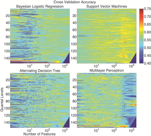
Fig. 1 illustrates the cross-validation accuracy for each of the four algorithms. To illustrate the full space, the F dimension is shown in log steps. On average, the SVM outperformed the other algorithms that otherwise seemed relatively indistinguishable. For extreme quantal levels, the accuracy of the MLP was comparable to the SVM. The maximum accuracy achieved was 86, 70, 69 and 71% for BLR, ADT, SVM and MLP, respectively. The minimum accuracy was 8, 32, 43 and 29% for BLR, ADT, SVM and MLP, respectively. The accuracy for a naive classifier in this setting is 56% (95% CI: 48-64%). Falsely assuming that the sampled points were randomly selected without replacement, the 95 percent confidence intervals for the mean cross validation accuracy for BLR, ADT, SVM and MLP were: 54.7-54.9; 54.0-54.2; 57.8-57.9 and55.5-55.7%.

Figure 1.

The cross validation accuracy of all four classifiers. The unsampled points are filled using Akima bivariate interpolation [6]. The bottom right corner is set to 0 due to lack of support. All values less than 40% are rounded up to 40% to maintain contrast. Without multiple testing correction, individual yellow to red points are significantly more accurate than a naive classifier whereas deep blue points are significantly worse.

A. Variance with respect to Feature Number

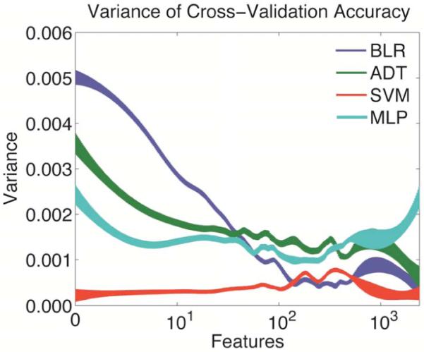
As illustrated in Fig. 2, the variance of accuracy of most algorithms decreases with increasing feature number. The notable exception is SVM, which had higher accuracy and lower variance across almost all of the space. The minimum for each algorithm was reached at 2,400; 2,400; 1 and 234 feature(s) for BLR, ADT, SVM and MLP, respectively.

Figure 2.

Variance of cross validation accuracy with respect to number of input features. Thickness represents standard error.

B. Variance with respect to Quantal Level

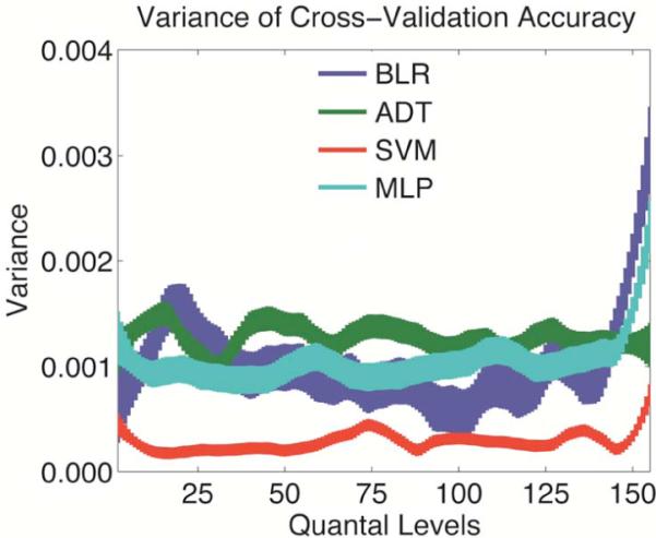
As illustrated in Fig. 3, the variance of accuracy is relatively constant except for high Q. The variance of SVM is lower than all algorithms across all selections.

Figure 3.

Variance of cross validation accuracy with respect to number of quantal levels. Thickness represents standard error.

IV. Discussion

We note a few key observations regarding the behavior of the cross-validation accuracy. (1) The distribution of all algorithms has substantial negative skew. (2) The number of features is responsible for most of the variation in accuracy. (3) The variance of cross-validation accuracy largely is independent of the choice of quantal level. (4) SVM has decreased variance and increased accuracy within this system compared to the other algorithms.

When visualizing the overall cross-validation accuracy (Fig. 1), the majority of points seem to be less than chance, 56%. This, however, is not the case. Negative bias occurs because the majority of points are sampled for low feature number relative to the optimum, causing these less accurate points to be over represented. This skew means that a naive or random choice of parameters could lead to a conclusion that no discriminatory signal exists when a signal indeed exists. This illustrates the need to better understand the effect of parameter selection.

It is apparent that as long as an intermediate number of quantal levels are chosen, the variance of accuracy is relatively constant. This suggests that the mRMR algorithm is resistant to small variations in the selection of this parameter and confirming our hypothesis that variance is decreased around the optimum Q. Even as the variance of accuracy is constant across quantal levels (Fig. 1), the accuracy is even more consistent within each quantal level.

Similarly, the variance with respect to number of features had very similar trends across the four algorithms. All of the algorithms achieved a local minimum of variance at around 200 to 500 features. This suggests that across all algorithms, this may represent the number of non-redundant features in the data that hold diagnostic information. As expected from the bias-variance tradeoff, the accuracy grows according to a roughly sigmoidal function that peaks around 500 features. After this optimum, the accuracy then falls, possibly due to over fitting, as discussed in the introduction. Due to the decreasing trend in variance for all but the MLP, it is not guaranteed that this represents a global optimum.

The magnitude of each of the variances suggests that on a large scale, the number of features is much more important than the choice of quantal level. Around the region with decreased variation in F, however, the variance from Q is of similar magnitude. This suggests that this space may be explored efficiently using coordinate descent.

It is particularly interesting to note the large difference in variance for low feature numbers. The most salient example is the BLR that has between 1.5 and 5 fold more variance for low F than the other algorithms. BLR achieves both the maximum and minimum global accuracy with low F and high Q, therefore this performance may be due to noise instead of (in)effective modeling of the underlying pathology or MI. This is confirmed by our hypothesis that with high Q the probability distribution of each feature approaches the uniform; therefore the MI calculation may be ineffective.

On the other hand, the SVM was impacted the least by the parameter selection. The variance with respect to both parameters was less for the SVM than for most of the other algorithms across all parameters. As discussed in the introduction, this may be because the underlying weighting of relevancy by mRMR is substantially different from the SVM. The minimum accuracy observed for the SVM was substantially higher than the minimum for all other algorithms. The optimum accuracy was also achieved across intermediate quantal levels, suggesting that it reflects an effective modeling of the underlying data to discriminate epilepsy from non-epileptic seizures. We caution against interpretation of the extrema because their significance can only be assessed using random field theory [6] and/or bias correction [7], both of which are out of scope for this article.

Based on these and other results, we believe that the power spectrum of EEG holds valuable diagnostic information for epilepsy but that this diagnostic information is hidden among a large degree of noise [8]. A deeper understanding of parameter selection may lead to the efficient implementation of power spectrum information on an automated diagnostic tool for epilepsy.

In general, a priori selection of the number of input features and quantal levels in mRMR has the same challenges as other feature selection algorithms even though it involves ajoint optimization because accuracy is generally invariant of quantal level. The selection of the optimum number of features requires sampling to determine the region that maximizes both classification accuracy and minimizes the variance with respect to changes in number of features. This ensures that the accuracy is not inflated artifactually but also correctly reports the best accuracy that can be achieved in practice.

References

- 1.Peng H, Long F, Ding C. Feature selection based on mutual information: criteria of max-dependency, max-relevance, and min-redundancy. IEEE Trans Pattern Analysis and Machine Intelligence. 2005;27(8):1226–38. doi: 10.1109/TPAMI.2005.159. [DOI] [PubMed] [Google Scholar]
- 2.Hall P, Morton SC. On the estimation of entropy. Ann Inst Statist Math. 1993;45(1):69–88. [Google Scholar]
- 3.Bouckaert RR, Frank E, Hall MA, Holmes G, Pfahringer B, Ruetemann P, Witten IH. Weka-experiences with a java open-source project. J Mach Learn Res. 2010;11:2533–41. [Google Scholar]
- 4.Akima H. Algorithm 761: scattered-data surface fitting that has the accuracy of a cubic polynomial. ACM Transactions on Mathematical Software. 1996;22:362–71. [Google Scholar]
- 5.Cleveland WS, Grosse E, Shyu WM. Chapter 8:Local regression models. In: Chambers JM, Hastie TJ, editors. Statistical Models. S: Wadsworth & Brooks/Cole; 1992. [Google Scholar]
- 6.Worsley KJ, Taylor JE, Tomaiuolo F, Lerch J. Unified univariate and multivariate random field theory. NeuroImage. 2004;23:S189–S95. doi: 10.1016/j.neuroimage.2004.07.026. [DOI] [PubMed] [Google Scholar]
- 7.Tibshirani RJ, Tibshirani R. A bias corection for the minimum error rate in cross-validation. Ann Appl Stat. 2009;3(2):822–9. [Google Scholar]
- 8.Sezer E, Isik H, Saracoglu E. Employment and comparison of different artificial neural networks for epilepsy diagnosis from EEG signals. J Med Syst. 2010;36(1):347–62. doi: 10.1007/s10916-010-9480-5. [DOI] [PubMed] [Google Scholar]