Multi‐atlas based representations for Alzheimer's disease diagnosis

Abstract

Brain morphometry based classification from magnetic resonance (MR) acquisitions has been widely investigated in the diagnosis of Alzheimer's disease (AD) and its prodromal stage, i.e., mild cognitive impairment (MCI). In the literature, a morphometric representation of brain structures is obtained by spatial normalization of each image into a common space (i.e., a pre‐defined atlas) via non‐linear registration, thus the corresponding regions in different brains can be compared. However, representations generated from one single atlas may not be sufficient to reveal the underlying anatomical differences between the groups of disease‐affected patients and normal controls (NC). In this article, we propose a different methodology, namely the multi‐atlas based morphometry, which measures morphometric representations of the same image in different spaces of multiple atlases. Representations generated from different atlases can thus provide the complementary information to discriminate different groups, and also reduce the negative impacts from registration errors. Specifically, each studied subject is registered to multiple atlases, where adaptive regional features are extracted. Then, all features from different atlases are jointly selected by a correlation and relevance based scheme, followed by final classification with the support vector machine (SVM). We have evaluated the proposed method on 459 subjects (97 AD, 117 progressive‐MCI (p‐MCI), 117 stable‐MCI (s‐MCI), and 128 NC) from the Alzheimer's Disease Neuroimaging Initiative (ADNI) database, and achieved 91.64% for AD/NC classification and 72.41% for p‐MCI/s‐MCI classification. Our results clearly demonstrate that the proposed multi‐atlas based method can significantly outperform the previous single‐atlas based methods. Hum Brain Mapp 35:5052–5070, 2014. © 2014 Wiley Periodicals, Inc.

INTRODUCTION

Morphometric pattern analysis is one of the most popular approaches for automatic Alzheimer's disease (AD) diagnosis. By directly accessing to the structures provided by magnetic resonance imaging (MRI), brain morphometry can be utilized to identify the anatomical differences between populations of AD patients and normal controls (NC), and subsequently determine the AD‐related characteristics to assist diagnosis, prognosis, as well as evaluation of mild cognitive impairment (MCI) progression and treatment effects.

Toward this goal, researchers have developed various techniques to measure brain morphometry. Most of the early works [Dickerson et al., 2001; Fox et al., 1996; Kaye et al., 1997; Killiany et al., 2000] resorted to direct volumetric measurements in predefined regions of interest (ROIs) (e.g., hippocampus, neocortex, or entorhinal cortex), and seek for the anatomical differences caused by AD or MCI in those specific regions. However, accurate reproduction of manually labeled ROIs is extremely difficult to perform across different subjects/data sets, and such prior knowledge of targeted disease is always limited. More recently, thanks to the substantial development of deformable image registration techniques in the last decade [Sotiras et al., 2013; Shen et al., 1999; Tang et al., 2009; Xue et al., 2006; Yap et al., 2009], automatic spatial normalization has become the fundamental step in morphometric pattern analysis, which allows quantitative comparison of different subjects/populations within a common space. Based upon the spatial normalization framework, voxel‐based morphometry (VBM) [Ashburner and Friston, 2000; Davatzikos et al., 2001, 1996; Thompson et al., 2001], deformation‐based morphometry (DBM) [Ashburner et al., 1998; Chung et al., 2001], and tensor‐based morphometry (TBM) [Fox et al., 2001; Freeborough and Fox, 1998; Riddle et al., 2004] have been proposed to characterize the brain shape, and demonstrated promising results in automatic AD diagnosis when combined with pattern classification techniques [Bozzali et al., 2006; Davatzikos et al., 2008; Fan et al., 2008c; Frisoni et al., 2002; Hua et al., 2008a,b; Lau et al., 2008; Teipel et al., 2007].

The VBM, DBM, and TBM methods are all performed by first spatially normalizing all subjects into a common atlas space. VBM‐type methods measure the local tissue density of the original brain volume directly, whereas DBM‐type methods and TBM‐type methods measure the deformation field and the Jacobian of deformation, respectively. Such measurements can then be regarded as features in conjunction with multivariate analysis (e.g., linear discriminant analysis or support vector machine, SVM), in order to perform MRI based classification. For example, based on the tissue density maps [Davatzikos, 1998; Davatzikos et al., 2001; Goldszal et al., 1998] generated from a mass‐preserving shape transformation framework [Shen and Davatzikos, 2003], Fan et al. [2007b] proposed the COMPARE algorithm (Classification Of Morphological Patterns using Adaptive Regional Elements) to extract volumetric features from the self‐organized, spatially adaptive local regions, for the purpose of overcoming the limitations of traditional voxel‐wise analysis (e.g., often with very high feature dimensionality and also significant measurement noise due to inter‐subject anatomical variations and registration errors) and thus enhancing the feature discriminative power. Because of its intrinsic advantages, COMPARE has been successfully applied to various MRI based applications, including schizophrenia classification [Fan et al., 2008a, 2007b], gender classification [Fan et al., 2008b], neurocognitive classification [Fan et al., 2007a], and AD classification [Fan et al., 2008c].

Nevertheless, traditional studies utilize only one atlas as the benchmark space to compare different groups of subjects. Recently, using multiple atlases for comparison of group difference has proven useful in reducing the negative impact of registration errors in morphometric analysis of brain MRI. For example, Leporé et al. [2008] proposed to register each image to multiple atlases (which have been spatially normalized to a common atlas by non‐linear registration) and then average the respective Jacobian maps (of the estimated deformation fields) to improve TBM based monozygotic/dizygotic twin classification. In addition to averaging the Jacobian maps, Koikkalainen et al. [2011] studied the effects of using mean deformation fields, mean volumetric features, and mean predicted responses (of regression‐based classifiers) from multiple atlases to reduce the variability caused by registration in the TBM based classification, and obtained the improved results for AD related analysis.

It is worth noting that in both Leporé et al. [2008] and Koikkalainen et al. [2011], the multiple atlases used for registration were non‐linearly aligned to a common space. As a result, anatomical structures of different atlases are similar to each other after nonlinear registration, and thus the morphometric patterns generated from those atlases for the same subject would be less effective at providing the complementary information. Although averaging outcomes from different atlases in different ways (e.g., averaging deformation fields, Jacobian maps, regional features, or classifier results as suggested in Koikkalainen et al. [2011]) can efficiently reduce errors caused by registration, it neglects the potentially important information related to anatomical differences between different atlases. Indeed, the anatomical structure of different atlases in their original (linearly‐aligned) spaces could be distinctive. Consequently, the morphometric patterns (e.g., VBM, DBM, or TBM) generated from different atlases in their original (linearly‐aligned) spaces can also be very different. To this end, we believe that aggregating patterns from multiple atlases can lead to a rich feature representation of each image and subsequently boost the discriminative power in classification. Figure 1 illustrates (1) how different morphometric patterns can be generated from different atlases via non‐linear transformation, where we show an example of the tissue density map of white matter (WM) calculated from the registration by HAMMER [Shen and Davatzikos, 2002], and (2) the amplified differences in comparison of two subjects when multiple atlases are jointly considered. Actually, the similar philosophy is widely applied in other domains. For example, a side‐view camera can capture the profile of an object, which is able to provide supplemental information for object recognition in addition to a frontal shot of the same object. In brain morphometry, multiple atlases can be similarly regarded as different “cameras” in such measurements for the same “object,” i.e., the brain MRI of an individual subject.

Figure 1.

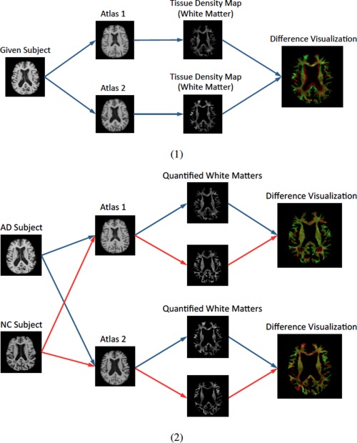
Illustration of different morphometric patterns generated from different atlases. (1) Registration of an image to different atlases leads to different representations. It can be seen that the geometrical structures of white matter (WM) represented in different atlases are different. In addition, tissue density distributions within each tissue are also different from the two different atlases. (2) Registration of different images (e.g., an AD subject and a NC subject) to different atlases: the differences between their representations from individual atlases are different (implying the amplified discriminative power when jointly considered in classification). [Color figure can be viewed in the online issue, which is available at http://wileyonlinelibrary.com.]

In this article, we propose to measure brain morphometry via multiple atlases, in order to generate a rich representation of anatomical structures that will be more discriminative to separate different groups of subjects. Unlike previous multi‐atlas based works [Koikkalainen et al., 2011; Leporé et al., 2008] which register their atlases to a common space via deformable registration, we retain the selected atlases in their original (linearly‐aligned) spaces without non‐linearly registering them to the common space, in order to consider different information provided by different atlases. In the proposed method, affinity propagation [Frey and Dueck, 2007] is first applied to select the most distinctive and representative atlases. Then, subjects from different groups are registered to different atlases by using HAMMER [Shen and Davatzikos, 2002]. By adopting a feature extraction method used in COMPARE [Fan et al., 2007b], the most discriminative regional features are subsequently extracted with respect to each atlas. Finally, we gather the most discriminative and robust features jointly from all different atlases by maximizing both feature relevance (w.r.t. the label information) and feature correlations from different atlases, and input them into the SVM for classification. The main contributions of this article can be summarized as follows:

• Multi‐atlas based morphometry is proposed to provide the complementary information for classification, in addition to its well‐known merit of reducing impacts of registration errors.

• A multi‐atlas based classification method is proposed for AD diagnosis.

• New atlas selection and feature selection methods are also proposed for this multi‐atlas based classification framework.

By performing 10‐fold cross validation with the ADNI database [Jack et al., 2008], we achieved significant performance improvement for AD/NC classification by using multiple atlases, and the convincing performance for p‐MCI/s‐MCI classification.

The rest of the article is organized as follows. We first describe the details of the proposed method in Methods section. Then, we illustrate the experiments and comparative results in Results section. We further discuss the pros/cons of the multi‐atlas based approach in Discussion section. Finally, we draw conclusions and elaborate on future research directions in Conclusion section.

METHODS

Preprocessing

A standard pre‐processing procedure is applied to the T1‐weighted MR brain images. First, non‐parametric non‐uniform bias correction (N3) [Sled et al., 1998] is applied to correct intensity inhomogeneity. Then, skull stripping [Wang et al., 2013, 2011] is performed, followed by manual review or correction to ensure the skull and dura have been cleanly removed. Next, cerebellum removal is conducted by warping a labeled atlas to each skull‐stripping image. Afterwards, each brain image is segmented into three tissues (gray matter (GM), white matter (WM), and cerebrospinal fluid (CSF)) by using FAST [Zhang et al., 2001], and finally all brain images are affine aligned by FLIRT [Jenkinson et al., 2002; Jenkinson and Smith, 2001].

Atlas Selection

Because our method utilizes multiple atlases for human brain representation in classification, the first question to address is how to select those multiple atlases. In [Koikkalainen et al., 2011], 30 atlases were randomly selected from different categories (10 for AD, 10 for MCI, and 10 for NC). However, the use of randomly selected atlases cannot guarantee to appropriately reflect the distribution of the whole population. Also, redundant information could be introduced with this random selection. Moreover, the selection of unrepresentative images as atlases could further cause large registration errors. To overcome these limitations, we propose a data‐driven atlas selection scheme to obtain the most distinctive and representative atlases.

In order to select atlases that can yield discriminative morphometric representations, differences among the selected atlases should be maximized. On the other hand, to reduce registration errors, the set of selected atlases should be representative enough to cover the entire population. To this end, we apply affinity propagation [Frey and Dueck, 2007] to partition the entire population (of AD and NC images) into T (e.g., $T=10$ in this article) nonoverlapping clusters. By performing affinity propagation, an exemplar image will be automatically selected for each cluster, which can then be used as a representative image or atlas for this cluster. By combining all exemplar images from all different clusters, we can obtain a set of atlases to form the atlas pool. During clustering, a bisection method [Frey and Dueck, 2007] is applied to find the appropriate preference value, and the image similarity is computed as normalized mutual information [Studholme et al., 1999]. The clustering results and the respective selected atlases from our experiments are shown in Figure 2. It should be noted that, although it is possible to add more atlases to the set of our selected atlases, those additional atlases could introduce the redundant information and thus affect the optimal representation of each subject.

Figure 2.

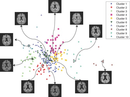
The clustering result of AD/NC subjects, using affinity propagation with normalized mutual information. Each selected atlas corresponds to an exemplar image of the respective cluster. Points are visualized by multidimensional scaling (MDS) [Kruskal, 1964]. [Color figure can be viewed in the online issue, which is available at http://wileyonlinelibrary.com.]

It should be noted that we only select atlases from the AD and NC subjects, but not from the MCI subjects. This is because MCI can be considered as an intermediate stage between AD and NC and thus associated with both AD and NC characteristics. In this article, we identify the morphormetrical patterns associated with the abnormality of AD (w.r.t. NC) and apply them to the p‐MCI/s‐MCI classification, which leads to more reliable classification results.

Registration and Quantification

The core steps in morphometric pattern analysis (e.g., VBM, DBM, or TBM) include (1) a registration step for spatial normalization of different images into a common space, and (2) a quantification step for morphometric measurement. Similar to [Fan et al., 2007b], a mass‐preserving shape transformation framework [Shen and Davatzikos, 2003] is adopted in our approach to capture the morphometric patterns of any given subject on the spaces of different atlases.

Figure 3 shows our registration and quantification steps. For a given subject with three segmented tissues (i.e., GM, WM, and CSF), the subject image is first registered to all T selected atlases by using a high‐dimensional elastic warping tool (i.e., HAMMER [Shen and Davatzikos, 2002]). Then, based on those T estimated deformation fields, for each tissue, we can quantify its voxel‐wise tissue density map in any of the T different atlas spaces. All these quantified tissue density maps [Davatzikos, 1998; Davatzikos et al., 2001; Goldszal et al., 1998] can thus reflect the unique deformation behaviors of the given subject with respect to each different atlas. In Figure 3, it is clear that the T generated tissue density maps are different in terms of both their density values and tissue structures, which lead to different feature representations, as introduced below.

Figure 3.

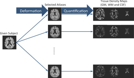
Registration and quantification of a subject registered to multiple atlases using HAMMER. Registration to different atlases leads to different quantification results. In the figure, the generated tissue density maps (GM, WM, and CSF) are different from registration via different atlases. [Color figure can be viewed in the online issue, which is available at http://wileyonlinelibrary.com.]

Since the gray matter (GM) is most affected by AD and thus widely investigated in the literature [Liu et al., 2012; Zhang and Shen, 2012; Zhang et al., 2011], in this article, the GM density map is used for feature extraction and classification.

Feature Extraction

We extract features from each atlas and then integrate them together for completely representing the subject brain by all atlases. To do this, in Watershed segmentation section, we first adaptively determine a set of ROIs in each atlas space by performing watershed segmentation [Grau et al., 2004; Vincent and Soille, 1991] on the correlation map obtained between the voxel‐wise tissue density values and class labels from all training subjects. Then, to improve both discrimination and robustness of the volumetric feature computed from each ROI, in Regional feature aggregation section, we further refine each ROI by picking only the voxels with reasonable representation power. Finally, to show the consistency and difference of ROIs obtained in all atlases, in Anatomical analysis section, we provide anatomical analysis for demonstrating the capability of our method in extracting the complementary features from multiple atlases for representing each subject brain.

Watershed segmentation

For robust feature extraction, it is important to group voxel‐wise morphometric features into regional features. Voxel‐wise morphometric features (such as the Jacobian determinants, voxel‐wise displacement fields, and tissue density maps) usually have very high feature dimensionality, which include a large amount of redundant/irrelevant information as well as noise due to registration errors. On the other hand, using regional features can alleviate the above issues and thus provide more robust features in classification.

A traditional way to obtain regional features is to use the prior knowledge, i.e., pre‐defined ROIs, to summarize all voxel‐wise features in each pre‐defined ROI. However, such method is inappropriate in our case of using multiple atlases for complementary representation of brain image, since in this way ROI features from multiple atlases will be very similar (we use the volume‐preserving measurement to calculate the atlas‐specific morphometric pattern of tissue density change within the same ROI w.r.t. each different atlases). In our method, we want to capture different sets of distinctive brain features from different atlases. Accordingly, we apply the clustering method in [Fan et al., 2007b] for adaptive feature grouping. Since clustering will be performed on each atlas space separately, the complementary information from different atlases can be preserved and obtained for the same subject image. In addition, as indicated in [Fan et al., 2007b], the clustering algorithm can also improve the discriminative power of the obtained regional features, and reduce the negative impacts from registration errors.

Let $I_i^t(u)$ denote a voxel‐wise tissue density value at voxel u in the t‐th atlas for the i‐th training subject, $i\in [1,N]$. ROI partition for the t‐th atlas is based on the combined discrimination and robustness measure, $DR{M}^t(u)$, computed from all N training subjects, which takes into account both feature relevance and spatial consistency as defined below:

$$DR{M}^t(u)=P^t(u)C^t(u)$$ (1)

where $P^t(u)$ is the voxel‐wise Pearson correlation between tissue density set $\{I_i^t(u),i\in [1,N]\}$ and label set $\{y_i\in [-1,1],i\in [1,N]\}$ (1 for AD and −1 for NC) from all N training subjects, and $C^t(u)$ denotes the spatial consistency among all features in the spatial neighborhood [Fan et al., 2007b].

Watershed segmentation is then performed on each calculated map $DR{M}^{\mathit{t}}$ for obtaining the ROI partitions for the t‐th atlas. Note that, before applying watershed segmentation, we use a Gaussian kernel to smooth each map $DR{M}^{\mathit{t}}$, to avoid any possible over‐segmentation, as suggested in [Fan et al., 2007b]. As a result, for example, we can partition the t‐th atlas into a total of $R^t$ non‐overlapping regions, $\{r_l^t,l\in [1,R^t]\}$, with each region $r_l^t$ owning $U_l^t$ voxels. It is worth noting that each atlas will yield its unique ROI partition, since different tissue density maps (of the same subject) are generated in different atlas spaces.

Figure 4 shows the partition results obtained from the same group of images registered to the two different atlases. It is clear that the obtained ROIs are very different, in terms of both their structures and discriminative powers (as indicated by different colors). Those differences will naturally guide the subsequent steps of feature extraction and selection, and thus provide the complementary information to represent each subject and also improve its classification.

Figure 4.

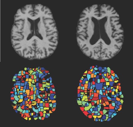
Watershed segmentation of the same group of subjects on two different atlases. Color indicates the discriminative power learned from the group of subjects (with the hotter color denoting more discriminative regions). Upper row: two different atlases. Lower row: the corresponding partition results. [Color figure can be viewed in the online issue, which is available at http://wileyonlinelibrary.com.]

Regional feature aggregation

Instead of using all $U_l^t$ voxels in each region $r_l^t$ for total regional volumetric measurement, we aggregate only a sub‐region ${\stackrel{\sim }{r}}_l^t$ in each region $r_l^t$ to further optimize the discriminative power of the obtained regional feature, by employing an iterative voxel selection algorithm. Specifically, we first select a most relevant voxel, according to the Pearson correlation calculated between this voxel's tissue density values and class labels from all N training subjects. Then, we iteratively include the neighboring voxels to increase the discriminative power of all selected voxels, until no increase is found when adding new voxels. Note that this iterative voxel selection process will finally lead to a voxel set (called as the optimal sub‐region) ${\stackrel{\sim }{r}}_l^t$ with ${\stackrel{\sim }{U}}_l^t$ voxels, which are selected from the region $r_l^t$. In this way, for a given subject i, its l‐th regional feature $V_{i,l}^t$ in the region ${\stackrel{\sim }{r}}_l^t$ of the t‐th atlas can be computed as:

$$V_{i,l}^t={\displaystyle {\sum }_{\forall u\in {\tilde{r}}_l^t}\frac{I_i^t(u)}{{\stackrel{\sim }{U}}_l^t}}$$ (2)

Each regional feature is then normalized to have zero mean and unit variance, across all N training subjects. Finally, from each atlas, M (out of $R^t$) most discriminative features are selected using their Pearson correlation. Thus, for each subject, its feature representation from all T atlases consists of $M\times T$ features, which will be further selected for classification as described in Section 2.5.

Figure 5 shows the top 100 regions selected using the regional feature aggregation scheme, for the same image registered to two different atlases (as shown in Fig. 4). It clearly shows the structural and discriminative differences of regional features from different atlases.

Figure 5.

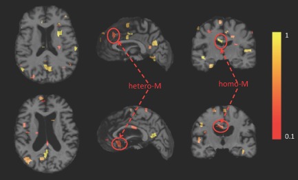
Illustration of the top 100 regions identified using the regional feature aggregation scheme, where the same subject is registered to two different atlases. The axial, sagittal and coronal views of the original MR image of the subject after warping to each of the two different atlases are displayed. Color indicates the discriminative power of the identified region (with the hotter color denoting more discriminative region). Upper row: image registered to atlas 1. Lower row: image registered to atlas 2. (For the definitions of both hetero‐M and homo‐M, please refer to Anatomical analysis section). [Color figure can be viewed in the online issue, which is available at http://wileyonlinelibrary.com.]

Anatomical analysis

It is important to understand how the identified regions (ROIs) from different atlases are correlated with the target brain abnormality (i.e., AD), in order to better reveal the advantages of using multiple atlases for morphometric pattern analysis in comparison to using only a single atlas. Accordingly, we categorize the identified regions (ROIs) into two classes: (1) the class with homogeneous measurements (homo‐M), and (2) the class with heterogeneous measurements (hetero‐M) (see Fig. 5). The homo‐M refers to the regions that are simultaneously identified from different atlases, whereas the hetero‐M refers to the regions identified in a certain atlas but not in other atlases. In Figure 5, it can be observed that a region within the left corpus callosum is identified in both atlas‐1 and atlas‐2 (see the coronal view). On the other hand, a region within the frontal lobe is only identified in atlas‐1, and a region within the temporal lobe is only identified in atlas‐2 (see the sagittal view). When jointly considering all identified regions from different atlases in the classification, the integration of homo‐M features is helpful to improve both robustness and generalization of feature extraction for the unseen subjects, while the combination of hetero‐M features can provide complementary information for distinguishing subjects during the classification.

Feature Selection

Although the most representative regional features are selected from each atlas, many regional features, after combined with other features from other atlases, could be redundant or even deteriorate the classification of unseen subjects. Therefore, selecting a subset of robust regional features (from all atlases) is an essential step to achieve good classification performance.

We have demonstrated via Figure 5 that the regional features identified from different atlases could be heterogeneous. Therefore, selecting features jointly from multiple atlases can potentially aggregate complementary information that is helpful for the classification. Specifically, for the N training images that have been registered to T atlases, all features extracted from T atlases can be denoted as $V=\left\{v_{n,m}^t,m\in \left[1,M\right],t\in \left[1,T\right], n\in \left[1,N\right]\right\}$, where M top selected features are extracted independently from each atlas by using the method described in Section 2.4.2. For each subject, i.e., the n‐th subject, its feature vector $V_n=\{v_{n,m}^t, m\in \left[1,M\right],t\in \left[1,T\right]\}$ has totally $\xi =M\times T$ features. Our goal here is to select the top K features, out of $\xi$ features, to gather the most discriminative and robust information jointly from all atlases. The detail of selecting the top K features is provided in the following paragraph.

Because the regional features extracted from different atlases are finally used for the same classification task, a “good” feature should be agreed not only by one atlas, but also by the other atlases. In other words, a “good” feature selected from one atlas should strongly correlate to the “good” features selected from the other atlases. Meanwhile, features that are helpful for classification should also strongly correlate with the training labels. To this end, in our feature selection, we propose to maximize both the feature relevance w.r.t. labels (i.e., according to the Pearson correlation), and the correlation with features from other atlases. This can be done by introducing the “inter‐atlas” correlation $\psi$, and combining it with the Pearson correlation $\omega$ by imposing a balancing factor $\lambda$ as follows:

$$\begin{array}{c}{\Delta }_m^t={\omega }_m^t+\lambda {\psi }_m^t\hfill \end{array}$$ (3)

where ${\Delta }_m^t$ indicates the importance of the $m$‐th feature computed from the $t$‐th atlas. The feature selection can then be achieved by ranking this feature importance for all $\xi =M\times T$ features, $\{{\Delta }_m^t,m\in [1,M],t\in [1,T]\}$. In Eq. (3), ${\omega }_m^t$ denotes the Pearson correlation between the m‐th feature from t‐th atlas and the class label from all training subjects. Similarly, the “inter‐atlas” correlation ${\psi }_m^t$ can be obtained by first computing the correlation between this m‐th feature in the t‐th atlas and each feature in other atlases, and then integrating all these correlation coefficients (via summation and normalization) as the final measure. By using the above scheme, we can select totally K top features with the highest feature importance values.

Classification

Linear support vector machine (SVM) [Cortes and Vapnik, 1995] is adopted to perform classification in our study. The choice of linear model is based on its good generalization capability across different training data (e.g., produced in each 10‐fold cross‐validation case in our experiments) [Burges, 1998].

RESULTS

Data

We use the Alzheimer's Disease Neuroimaging Initiative (ADNI) database to evaluate the performance of the proposed classification algorithm. The primary goal of ADNI has been to test whether serial magnetic resonance imaging (MRI), positron emission tomography (PET), other biological markers, and clinical and neuropsychological assessment can be combined to measure the progression of mild cognitive impairment (MCI) and early Alzheimer's disease (AD). Determination of sensitive and specific markers of very early AD progression is intended to aid researchers and clinicians to develop new treatments and monitor their effectiveness, as well as lessen the time and cost of clinical trials.

Since we focus on the morphometric study of AD, T1‐weighted MRI data from ADNI [Jack et al., 2008] is used in our experiments. In total, 459 subjects, scanned with 1.5T scanner, are randomly selected, which are comprised of 97 AD, 128 NC, and 234 MCI (117 p‐MCI and 117 s‐MCI) subjects. The demographic information of the used dataset is shown in Table 1.

Table 1.

Demographic information of the studied subjects (from ADNI database)

Diagnosis	Number	Age	Gender (M/F)	MMSE
AD	97	75.90±6.84	48/49	23.37±1.84
p‐MCI	117	75.18±6.97	67/50	26.45±1.66
s‐MCI	117	75.09±7.65	79/38	27.42±1.78
NC	128	76.11±5.10	63/65	29.13±0.96

The values are denoted as mean ± standard deviation.

It is worth noting that we did not use all subjects from ADNI, considering the long processing time for registering all subjects to the multiple (10) atlases, since the purpose of this study is to develop a new disease diagnosis method. On the other hand, the size of dataset used in our experiments is similar to that used in many previous studies [Cuingnet et al., 2011; Koikkalainen et al., 2011; Zhang et al., 2011]; thus it is sufficient for us to compare across different methods in this article, especially for the classification results obtained with single atlas and multiple atlases in the literature.

Evaluation Protocol

The evaluation of our method is conducted on two different problems: (1) AD diagnosis such as AD/NC classification, and (2) progressive MCI diagnosis such as p‐MCI/s‐MCI classification. The second problem is considered more difficult than the first problem, but has received relatively less attention in the previous studies. However, it is important to identify progressive MCI patients from the stable MCI patients, in order to possibly prevent the progression of MCI to AD via timely therapeutic interventions.

In our experiments, we use 10‐fold cross validation to both extract ROIs in each atlas space and evaluate the classification performance in the two above‐mentioned problems. Specifically, we make a random partition of all AD, NC, and MCI data (including p‐MCI and s‐MCI data) into 10 folds (each fold with roughly equal size). In each round, one fold of the data is used for testing, and the other nine folds are used for training. The final result is computed as the average score across all 10 cross‐validations. It should be noted that we conduct p‐MCI/s‐MCI classification in a transfer‐learning manner. That is, we use the abnormal patterns identified between AD and NC for guiding the p‐MCI/s‐MCI classification. Specifically, the way of identifying regional features and also the training of the SVM classifier are both conducted on the AD/NC data, and then the final protocol is directly applied to classify p‐MCI and s‐MCI subjects, by associating p‐MCI with the AD label and s‐MCI with the NC label. Note that, within the 10‐fold cross validation framework, nine folds of the AD/NC data are used for training, and the trained classifier is applied to one corresponding fold of the p‐MCI/s‐MCI data for testing.

We also use the same parameter values for all experiments in this article. Specifically, 10 representative atlases are selected from all AD/NC data by using the method described in Atlas Selection section. The top $M=1500$ regional features are extracted from each atlas, before conducting the joint selection of features from all different atlases. The balancing factor $\lambda$ is set to 0.38. Note that the selection of parameters M and $\lambda$ is based on cross‐validation results. The SVM classifier used in our method is implemented by the LIBSVM library [Chang and Lin, 2011], using a linear kernel and $C=1$ (the default cost). Finally, $K=1:1500$ features are tested, and the best results are reported for quantitative comparison.

AD Classification

Classification using single atlas

We first show the results using single atlas for AD/NC classification, to demonstrate the variability of classification results when using different atlases even for the same classification task. Because the proposed feature selection method integrates not only the Pearson correlation but also the “inter‐atlas” correlation from the multiple atlases, in this section, we thus examine two other conventional feature selection methods based on single atlas. The first feature selection method is simply based on the ranking of Pearson correlation (PC), and the second method combines PC with SVM‐RFE based feature selection [Guyon et al., 2002] (as proposed in Fan et al. [2007b] for jointly considering multiple features in the selection. It should be noted that, in the single atlas case, the feature extraction performed in our method is same as COMPARE [Fan et al., 2007b]. Therefore, in this article, we denote the PC+SVM‐RFE based method using single atlas as COMPARE. Figure 6 shows the classification performance by PC (Fig. 6(1)) and COMPARE (Fig. 6(2)) using 10 different atlases obtained from our selected atlas pool. Each curve shows the classification performance with respect to the use of different number of top selected features.

Figure 6.

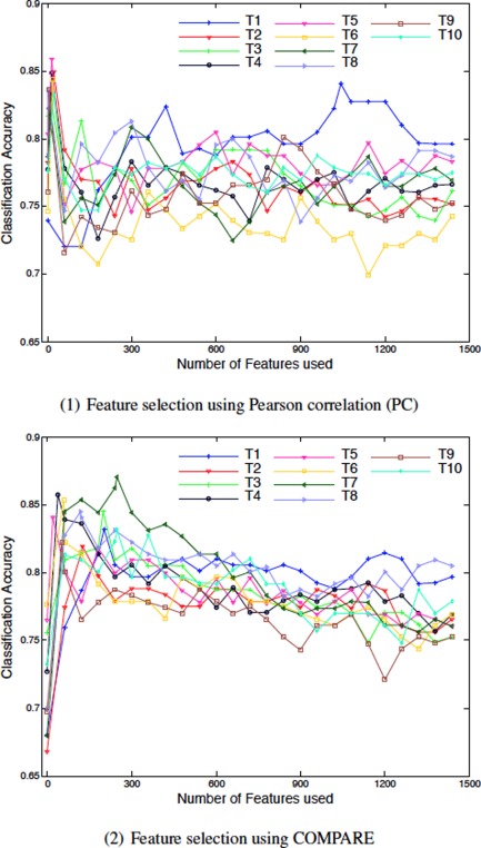
Results of AD/NC classification based on single atlas (T1‐T10). [Color figure can be viewed in the online issue, which is available at http://wileyonlinelibrary.com.]

As can be seen in the figure, results obtained from 10 different atlases (T1‐T10) are very different. For the PC based method, T1 gives the best overall classification performance, whereas, for COMPARE, T7 is the best atlas in comparison to the other atlases. The good performance from a specific atlas (for example T7) could be due to multiple reasons. First, its anatomical structures may be more representative for the entire population than the other atlases, so that the overall registration errors to T7 are smaller and thus the data representations generated by T7 are less noisy. Second, the deformation fields estimated from different (training) images to T7 could be more discriminative for identifying the AD‐related patterns than those to the other atlases. Finally, the AD‐related patterns identified by T7 may have better generalization capability to the testing subjects than the other atlases. By considering all the above possible reasons, respectively related to registration error, discriminative power, and generalization capability, one atlas could yield better classification accuracy than other atlases for a specific classification task or a specific data set. On the other hand, it should be noted that the accuracy typically decreases rapidly when including more features, even using the best atlas. This phenomenon indicates that many of the selected features from a single atlas could be redundant and noisy for classification.

In Table 2, we give the best classification accuracies (ACC) for each of the 10 atlases using PC and COMPARE, along with their respective sensitivities (SEN) and specificities (SPEC). The sensitivity and the specificity refer to the portions of correctly identified AD patients and correctly classified NC subjects, respectively. From the table, it is clear that COMPARE outperforms PC when using their own best atlases (i.e., T5 for PC, and T7 for COMPARE). These results are consistent with those reported in [Fan et al., 2007b]. However, for some atlases (i.e., T1, T2, T5, T9, and T10), the use of additional SVM‐RFE based feature selection (in COMPARE) cannot further improve the simple PC based classification (in terms of the best classification accuracy). That is, the result improvement brought by SVM‐RFE is limited, but at a cost of increased computational burden.

Table 2.

Results of AD/NC classification and p‐MCI/s‐MCI classification using different atlases (T1‐T10)

Atlas	AD/NC classification						p‐MCI/s‐MCI classification
	PC			COMPARE			PC			COMPARE
	ACC (%)	SEN (%)	SPEC (%)	ACC (%)	SEN (%)	SPEC (%)	ACC (%)	SEN (%)	SPEC (%)	ACC (%)	SEN (%)	SPEC (%)
T1	84.09	78.33	88.40	83.16	75.33	89.17	68.93	64.62	73.18	71.03	68.79	73.18
T2	84.94	80.56	88.33	81.95	73.67	88.40	68.87	68.56	69.09	71.46	71.97	70.76
T3	83.12	77.33	87.56	84.50	78.44	89.17	69.34	65.15	73.41	69.81	69.47	70.08
T4	84.87	80.44	88.33	85.72	82.22	88.40	72.71	73.56	71.82	71.82	72.58	71.06
T5	85.85	82.56	88.46	84.05	76.22	90.00	70.66	69.39	71.82	71.93	71.21	72.80
T6	84.38	78.33	89.04	85.35	83.56	86.73	71.04	65.98	75.98	72.86	69.62	76.14
T7	82.23	77.22	86.09	87.07	81.33	91.54	71.08	73.94	68.18	74.56	70.38	78.64
T8	83.59	79.44	86.86	84.48	79.44	88.46	70.27	68.71	71.67	71.88	68.56	75.00
T9	83.65	77.33	88.40	82.27	78.44	85.38	68.55	66.36	70.68	71.10	66.97	75.15
T10	83.28	83.78	83.01	83.20	76.56	88.46	69.00	72.05	65.83	71.74	70.15	73.41

ACC=accuracy, SEN=sensitivity, SPEC=specificity, AUC= area under curve.

Classification using multiple atlases

In this section, we show the results of AD/NC classification using multiple atlases. The proposed (multi‐atlas based) feature selection method (namely MA_Proposed) that considers both Pearson correlation and “inter‐atlas” correlation is compared with both PC and COMPARE based feature selection methods using either single atlas (namely SA_PC and SA_COMPARE) or multiple atlases (namely MA_PC and MA_COMPARE). For fair comparison, we average the classification results of single atlas based methods (SA_PC and SA_COMPARE) across all 10 atlases. We then directly extend these two methods to our multiatlas based framework as described below, and denote them as MA_PC and MA_COMPARE. Specifically, in MA_PC, all regional features extracted from 10 different atlases are used, thus resulting in a feature representation with $M\times T=15000$ dimensions for each subject; afterwards, the top 1,500 features are selected out of 15,000 features based on the Pearson correlation, and $K=1:1500$ features are subsequently selected and used for classification. In MA_COMPARE, the top 1,500 features are first selected in the same way as MA_PC, but additionally using SVM‐RFE to further refine the selected features, before inputting them to the SVM for classification. Figure 7 illustrates the results of SA_PC, SA_COMPARE, MA_PC, MA_COMPARE, and MA_Proposed (our proposed method) for AD/NC classification w.r.t. different numbers of top selected features.

Figure 7.

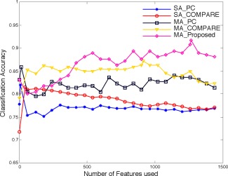
Results of SA_PC, SA_COMPARE, MA_PC, MA_COMPARE, and MA_Proposed for AD/NC classification. [Color figure can be viewed in the online issue, which is available at http://wileyonlinelibrary.com.]

In the figure, it is clear that the results of multiatlas based methods (MA_PC, MA_COMPARE, and MA_Proposed) outperform the results of single‐atlas based methods (SA_PC and SA_COMPARE) by a significant margin. Specifically, SA_PC and SA_COMPARE reach their best classification accuracy with a small portion of top selected features and then decline in performance rapidly when more features are included. This indicates that many of their selected features are noisy and redundant, if using only single atlas. In contrast, multi‐atlas based methods consistently improve or maintain their performance with the increase of the number of features used, which demonstrates that the complementary information from different atlases are aggregated together to improve the classification. In addition, with the assistance of SVM‐RFE, the COMPARE based methods (SA_COMPARE and MA_COMPARE) achieve better performance than the PC based methods (SA_PC and MA_PC) in both cases of using single atlas and multiple atlases. Figure 7 also clearly demonstrates that the proposed method significantly outperforms all other comparison methods. Although only a small portion of features can give good classification accuracy for the single atlas based methods, the performance of the proposed method is consistently improved when using more features (i.e., $91.64\%$ when using $K=1268$ features). This phenomenon shows that the redundant features from a single atlas can be integrated with the features from other atlases (in an effective way) to yield more robust and discriminative representations.

The best classification accuracies (ACC) as well as the corresponding sensitivities (SEN) and specificities (SPEC) of all methods are illustrated in Table 3. In addition, we also report the area under curve (AUC) rate. The results clearly show that the proposed method is better than any other methods in terms of all metrics. It should be noted that the sensitivities of SA_PC, SA_COMPARE, MA_PC, and MA_COMPARE are much lower in comparison to their corresponding specificities. Low sensitivity value indicates low confidence on AD diagnosis, which will greatly limit their practical usage. On the other hand, the proposed method gives a significantly improved sensitivity value, i.e., $8\%$ higher than the second best method. Together with its high specificity ( $93.85\%$), the proposed method produces more confident AD diagnosis results.

Table 3.

Results of AD/NC classification using single atlas (SA_PC, SA_COMPARE) and multiple atlases (MA_PC, MA_COMPARE, MA_Proposed)

Method	ACC (%)	SEN (%)	SPEC (%)	AUC (%)
SA_PC	82.01	75.88	86.76	76.92
SA_COMPARE	81.52	77.11	84.92	78.70
MA_PC	85.91	81.56	89.23	81.91
MA_COMPARE	87.19	80.56	92.31	84.95
MA_Proposed	91.64	88.56	93.85	86.75

ACC = accuracy, SEN = sensitivity, SPEC = specificity.

MCI Classification

Classification using single atlas

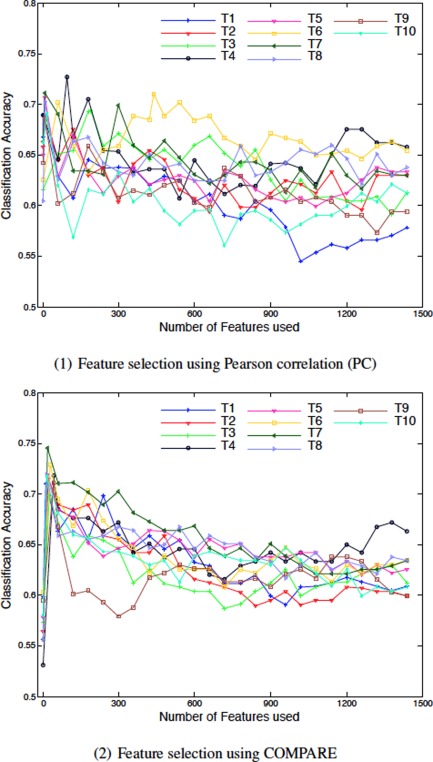
The single‐atlas based methods are also evaluated for p‐MCI/s‐MCI classification. Figure 8 shows the classification accuracy of both PC and COMPARE methods, w.r.t. different number of the top selected features. It can be seen that the classification results are much lower than those for AD/NC classification, since p‐MCI/s‐MCI classification is a difficult task in automatic morphometric analysis and clinical diagnosis. This is because the disease is still in the early stage, and the related atrophy is small and thus not effective for distinguishing between p‐MCI and s‐MCI subjects [Suk H‐IaL et al., 2013; Wee et al., 2011; Wee et al., 2012]. Similar to the results of AD/NC classification, there exists a large variation of accuracy for the use of different atlases. For the PC based method, T4 maintains a good performance in comparison to the other atlases, whereas T7 is the best atlas for the COMPARE based method in p‐MCI/s‐MCI classification (which is similarly observed in AD/NC classification, as described in Classification using single atlas section). The classification accuracy of the COMPARE based method using T7 reaches its maximum quickly when using only $K=120$ features, and then drops down drastically to 61.28% when incorporating more other features.

Figure 8.

Results of p‐MCI/s‐MCI classification based on single atlas (T1‐T10). [Color figure can be viewed in the online issue, which is available at http://wileyonlinelibrary.com.]

Table 2 also reports the best results (i.e., the best ACC, along with the corresponding SEN and SPEC) of both PC and COMPARE based methods for p‐MCI/s‐MCI classification. The results clearly show that the COMPARE based method outperforms the PC based method. In particular, the atlas T7 yields much higher performance than all other atlases, potentially due to its low registration error, superb discriminative power, and good generalization capability as mentioned above. However, in practice, finding such a ideal atlas is always a difficult task.

Classification using multiple atlases

We compare the performances of five methods, i.e., SA_PC, SA_COMPARE, MA_PC, MA_COMPARE and MA_Proposed, for the case of p‐MCI/s‐MCI classification, as shown in Figure 9. From Figure 9, we can observe again that all three multi‐atlas based methods (MA_PC, MA_COMPARE, and MA_Proposed) perform significantly better than the two single‐atlas based methods (SA_PC, SA_COMPARE), indicating the power of using multiple atlases in aggregating more useful information for classification. Among all three multi‐atlas based methods, the proposed method (MA_Proposed) demonstrates comparable performance to both MA_PC and MA_COMPARE. When using the $K=500:1000$ top selected features, the proposed method (MA_Proposed) gives the best overall classification results. On the other hand, MA_COMPARE gets its best results when using $K=1:500$ features, and MA_PC achieves its best results when using $K=1000:1500$ features, respectively.

Figure 9.

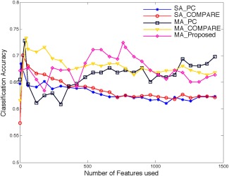
Results of SA_PC, SA_COMPARE, MA_PC, MA_COMPARE, and MA_Proposed for p‐MCI/s‐MCI classification. [Color figure can be viewed in the online issue, which is available at http://wileyonlinelibrary.com.]

We also show the best classification performance of each method in Table 4. As we can see from Table 4, all three multi‐atlas based methods demonstrate better performance than the single atlas based methods. Specifically, MA_COMPARE obtains both the best classification accuracy and the highest sensitivity value, while the proposed method (MA_Proposed) yields the best specificity value. Note that the high specificity value of the proposed method can potentially reduce the misdiagnosis rate of stable MCI patients.

Table 4.

Results of p‐MCI/s‐MCI classification using single atlas (SA_PC, SA_COMPARE) and multiple atlases (MA_PC, MA_COMPARE, MA_Proposed)

	ACC	SEN	SPEC	AUC
Method	(%)	(%)	(%)	(%)
SA_PC	68.49	67.80	69.10	62.85
SA_COMPARE	70.06	68.08	72.02	63.56
MA_PC	72.78	74.62	70.91	66.45
MA_COMPARE	73.35	75.76	70.83	67.98
MA_Proposed	72.41	72.12	72.58	67.37

ACC = accuracy, SEN = sensitivity, SPEC = specificity, AUC = area under curve.

Comparison With Existing Classification Methods

In this section, we compare our results with the four recently reported methods on AD diagnosis, based on either single atlas [Cuingnet et al., 2011; Liu et al., 2012; Zhang et al., 2011] or multiple atlases [Koikkalainen et al., 2011], demonstrating the superiority of the proposed method. For fair comparison, only the results based on MRI data are reported from the multimodality based approach in [Zhang et al., 2011]. Tables 5 and 6 present the comparative results for AD/NC classification and p‐MCI/s‐MCI classification, respectively. Details of each method are given in the tables, which include the type of features, classifier, and subjects used.

Table 5.

Comparison to existing works using MRI data of ADNI for AD/NC classification

Method	Feature	Classifier	Subjects	Atlas	ACC (%)	SEN (%)	SPEC (%)
Cuingnet et al. [2011]	Voxel‐Direct‐D GM	SVM	137 AD + 162 NC	Single‐atlas	88.58	81.00	95.00
Zhang et al. [2011]	93 ROI GM	SVM	51 AD + 52 NC	Single‐atlas	86.20	86.00	86.30
Liu et al. [2012]	Voxel‐wise GM	SRC ensemble	198 AD + 229 NC	Single‐atlas	90.80	86.32	94.76
Koikkalainen et al. [2011]	TBM	Linear regression	88 AD + 115 NC	multi‐atlas	86.00	81.00	91.00
Proposed method	Data‐driven ROI GM	SVM	97 AD + 128 NC	multi‐atlas	91.64	88.56	93.85

Table 6.

Comparison to existing works using MRI data of ADNI for p‐MCI/s‐MCI classification

Method	Feature	Classifier	Subjects	Atlas	ACC (%)	SEN (%)	SPEC (%)
Cuingnet et al. [2011]	Voxel‐STAND‐DGM	SVM	76 p‐MCI + 134 s‐MCI	Single‐atlas	70.40	57.00	78.00
Koikkalainen et al. [2011]	TBM	Linear regression	54 p‐MCI + 115 s‐MCI	Multi‐atlas	72.10	77.00	71.00
Proposed method	Data‐driven ROI GM	SVM	117 p‐MCI + 117 s‐MCI	Multi‐atlas	72.41	72.12	72.58

Data used in preparation of this article were obtained from the Alzheimer's Disease Neuroimaging Initiative (ADNI) database (http://www.loni.ucla.edu/ADNI). As such, the investigators within the ADNI contributed to the design and implementation of ADNI and/or provided data but did not participate in analysis or writing of this report. A complete listing of ADNI investigators can be found at: http://www.loni.ucla.edu/ADNI/Collaboration/ADNI_Authorship_list.pdf.

For AD/NC classification, the proposed method outperforms all other comparison methods, in terms of both classification accuracy and sensitivity. Only the method proposed by [Liu et al., 2012] obtained the comparable classification result (90.80%) to our method (91.64%), which has higher specificity value than ours. Although [Cuingnet et al., 2011] reported the highest specificity value, their sensitivity value is very low. On the other hand, our multi‐atlas based method significantly outperforms the multi‐atlas based method proposed by [Koikkalainen et al., 2011], which achieved its best accuracy by averaging the feature vectors from different atlases. Among all the comparison methods, only [Cuingnet et al., 2011] and [Koikkalainen et al., 2011] reported their performances for the more difficult task, i.e., p‐MCI/s‐MCI classification. Therefore, we listed their performances along with ours in Table 6. Note that in [Cuingnet et al., 2011], the best results for AD/NC classification and p‐MCI/s‐MCI classification were obtained using different features, i.e., directly using the tissue density map of GM for AD/NC classification, while using a subset of features selected by the method in [Vemuri et al., 2008] for p‐MCI/s‐MCI classification. On the other hand, in [Koikkalainen et al., 2011], the best p‐MCI/s‐MCI classification accuracy was obtained using a strategy that is different from that used in AD/NC classification. Specifically, instead of averaging the feature vectors from different atlases, the best result for p‐MCI/s‐MCI classification was achieved by combining the classifiers trained from different atlases. Finally, even if both [Cuingnet et al., 2011] and [Koikkalainen et al., 2011] applied different methods for AD/NC classification and p‐MCI/s‐MCI classification, respectively, their AD/NC classification results are still much lower than ours (Table 5). Also, for p‐MCI/s‐MCI classification (Table 6), the proposed method gives better classification accuracy than both [Cuingnet et al., 2011] and [Koikkalainen et al., 2011], although we used the same features and same classification strategy as in AD/NC classification.

DISCUSSION

In this article, we have developed a novel multi‐atlas based classification method for adaptively extracting the complementary regional features from multiple atlases for helping AD diagnosis. The results on 459 ADNI subjects demonstrated the consistent and substantial improvements by using our multi‐atlas based morphometric patterns. Specifically, our approach achieves high accuracy for AD/NC classification (91.64%) along with significantly improved sensitivity (88.56%), and also obtains the relatively high accuracy for p‐MCI/s‐MCI classification (72.41%) in comparison to a number of state‐of‐the‐art methods.

Comparison With the Baseline Method

Results by our method have been extensively compared with its baseline method—the COMPARE algorithm, in order to demonstrate the advantage of using multi‐atlas idea in AD diagnosis. COMPARE uses a single atlas for AD diagnosis, and achieved 87.05% accuracy when using the best atlas. Note that the classification accuracy we obtained is not as good as the best accuracy (94%) reported in [Fan et al., 2008c]. Actually, our obtained result for COMPARE is consistent with some recent results in [Cuingnet et al., 2011] and [Liu et al., 2012]. In [Cuingnet et al., 2011], the authors contributed these different results to the use of different data and different pre‐processing steps. Liu et al. [2012] argued that the adaptive feature extraction method introduced by COMPARE is difficult to robustly identify the discriminative regions for large population (as the case in our application).

It is worth noting that the purpose of this article is not to improve COMPARE's performance, but to demonstrate that the use of multiple atlases can significantly improve the classification performance. To this end, we have compared different feature selection strategies, i.e., Pearson correlation (PC), PC + SVM‐RFE, and the proposed feature selection that integrates PC and the “inter‐atlas” correlation from multiple atlases. Our results have justified that the multi‐atlas based methods performed much better than the single atlas based methods. In particular, when using multiple atlases, the proposed feature selection method achieved the best accuracy (91.64%) for AD/NC classification, while the feature selection method used in COMPARE achieved the best accuracy (73.35%) for p‐MCI/s‐MCI classification. All these results significantly outperformed those obtained by the baseline method—COMPARE using the single atlas.

Effect of Atlas Selection

Atlas is used as the common space to register different subjects for morphometric comparison. Selection of such an atlas has been pursued in different ways in the literature. The atlas can be an image of a single subject from the studied population [Cuingnet et al., 2011; Leporé et al., 2008], a general anatomical model, or the mean model generated from the studied population [Hua et al., 2008a,b; Leporé et al., 2007; Teipel et al., 2007]. The mean model is popularly used in order to reduce the registration errors by decreasing the overall distance from all subjects to the common space. Nevertheless, Leporé et al. [2008] argued that the anatomical boundaries and image gradients are often much blurrier in the mean model, which may reduce the accuracy of the registration. Therefore, they used multiple atlases for registration and then averaged the generated Jacobian maps to improve the classification. In our experiments, different atlases led to significantly different classification performances. Instead of choosing an optimal atlas from a set of atlases, we used all atlases for the complementary feature representation of each subject and thus obtained better performance than the use of even the best atlas in AD/NC classification.

On the other hand, Koikkalainen et al. [2011] also used multiple atlases that were randomly selected for registration. However, this random selection scheme might lead to more registration errors if outlier atlases are selected, and will also introduce extra redundancy in multi‐atlas based representation if some atlases are very similar. Our data‐driven method based on affinity propagation as detailed in Atlas Selection section can effectively overcome these limitations.

Effect of Feature Selection

It is well known that feature selection plays a key role in achieving robust classification accuracy. In [Fan et al., 2007b], SVM‐RFE based feature selection was integrated with Pearson correlation (PC) based feature selection to obtain the improved classification results. However, in the case of multi‐atlas based analysis, the feature representations obtained from different atlases bring not only complementary information, but also potentially redundant features. Therefore, feature selection must be carefully designed, in order to retrieve the most important/relevant information jointly from all different atlases. In our experiments, the PC based method can achieve 85.91% for AD/NC classification and 72.78% for p‐MCI/s‐MCI classification, but its improvements w.r.t. the use of single atlas are limited. The PC + SVM‐RFE based method can improve more accuracy in both classification cases, i.e., achieved the best performance of 73.35% for p‐MCI/s‐MCI classification. By selecting the “consensus” features jointly from all different atlases in addition to their relevance with the label information, the proposed feature selection method is able to increase the classification accuracy by a significant margin, i.e., 4.45% from PC + SVM‐RFE for the case of using multiple atlases and 10.12% from PC+SVM‐RFE for the case of using single atlas for AD/NC classification.

Limitations

It is worth indicating that our method exhibits higher computational cost because of using multiple atlases for image registration, e.g., with HAMMER [Shen and Davatzikos, 2002]. One solution is to parallelize the registration procedure by using multiple CPUs. Another possibility is to build a graph/tree based structure [Jia et al., 2010] for the atlas pool to guide the registration. In addition, the registration method (HAMMER) adopted in our article could be replaced by some less expensive techniques, e.g., diffeomorphic demons [Vercauteren et al., 2009], which may accelerate the registration process.

CONCLUSION

To conclude, we have developed a multi‐atlas based feature representation, selection, and classification method for AD diagnosis. Instead of registering subjects to a single atlas space, we registered each subject to multiple atlases selected by affinity propagation, and then extracted the morphometric patterns separately from each atlas for the complementary feature representation of each subject. By jointly considering the regional information from all atlases, the most discriminative and robust features can be finally identified by maximizing both feature correlation and feature relevance obtained from multiple atlases. The 10‐fold cross validation results on ADNI database have revealed the superiority of the proposed multi‐atlas based method over the single‐atlas based method in AD diagnosis.

In the current article, we evaluated our method based on the regional features computed from COMPARE algorithm. Other morphometric features, such as Jacobian determinants, can also be incorporated into our framework, which will be our future work. In addition, diverse classification strategies, such as linear regression, random forest, and sparse classification, can be applied, instead of using only SVM as in our current work, which could potentially yield better results. Finally, the current method can also be extended to other brain disease diagnosis applications, such as schizophrenia and autism diagnosis.

REFERENCES

- Ashburner J, Friston KJ (2000): Voxel‐based morphometry‐The methods. Neuroimage 11:805–821. [DOI] [PubMed] [Google Scholar]
- Ashburner J, Hutton C, Frackowiak R, Johnsrude I, Price C, Friston K (1998): Identifying global anatomical differences: deformation‐based morphometry. Hum Brain Mapp 6:348–357. [DOI] [PMC free article] [PubMed] [Google Scholar]
- Bozzali M, Filippi M, Magnani G, Cercignani M, Franceschi M, Schiatti E, Castiglioni S, Mossini R, Falautano M, Scotti G, et al. (2006): The contribution of voxel‐based morphometry in staging patients with mild cognitive impairment. Neurology 67:453–460. [DOI] [PubMed] [Google Scholar]
- Burges CJC (1998): A tutorial on support vector machines for pattern recognition. Data Min Knowl Discov 2:121–167. [Google Scholar]
- Chang C‐C, Lin C‐J (2011): LIBSVM: A library for support vector machines. ACM Trans. Intell. Syst Technol 2:27:1–27:27. [Google Scholar]
- Chung MK, Worsley KJ, Paus T, Cherif C, Collins DL, Giedd JN, Rapoport JL, Evans AC (2001): A unified statistical approach to deformation‐based morphometry. Neuroimage 14:595–606. [DOI] [PubMed] [Google Scholar]
- Cortes C, Vapnik V (1995): Support‐vector networks. Mach Learn 20:273–297. [Google Scholar]
- Cuingnet R, Gerardin E, Tessieras J, Auzias G, Lehéricy S, Habert M‐O, Chupin M, Benali H, Colliot O (2011): Automatic classification of patients with Alzheimer's disease from structural MRI: A comparison of ten methods using the \ADNI\ database Neuroimage 56:766–781. [DOI] [PubMed] [Google Scholar]
- Davatzikos C (1998): Mapping image data to stereotaxic spaces: Applications to brain mapping. Hum Brain Mapp 6:334–338. [DOI] [PMC free article] [PubMed] [Google Scholar]
- Davatzikos C, Fan Y, Wu X, Shen D, Resnick SM (2008): Detection of prodromal Alzheimer's disease via pattern classification of magnetic resonance imaging. Neurobiol Aging 29:514–523. [DOI] [PMC free article] [PubMed] [Google Scholar]
- Davatzikos C, Genc A, Xu D, Resnick SM (2001): Voxel‐based morphometry using the \ravens\ maps: Methods and validation using simulated longitudinal atrophy Neuroimage 14:1361–1369. [DOI] [PubMed] [Google Scholar]
- Davatzikos C, Vaillant M, Resnick SM, Prince JL, Letovsky S, Bryan RN (1996): A computerized approach for morphological analysis of the corpus callosum. J Comput Assist Tomogr 20:88–97. [DOI] [PubMed] [Google Scholar]
- Dickerson BC, Goncharova I, Sullivan MP, Forchetti C, Wilson RS, Bennett DA, Beckett LA, deToledo‐Morrell L (2001): MRI‐derived entorhinal and hippocampal atrophy in incipient and very mild Alzheimer's disease. Neurobiol Aging 22:747–754. [DOI] [PubMed] [Google Scholar]
- Fan Y, Gur RE, Gur RC, Wu X, Shen D, Calkins ME, Davatzikos C (2008a): Unaffected family members and schizophrenia patients share brain structure patterns: A high‐dimensional pattern classification study. Biol Psychiatry 63:118–24. [DOI] [PMC free article] [PubMed] [Google Scholar]
- Fan Y, Rao H, Hurt H, Giannetta J, Korczykowski M, Shera D, Avants BB, Gee JC, Wang J, Shen D (2007a): Multivariate examination of brain abnormality using both structural and functional MRI. Neuroimage 36:1189–1199. [DOI] [PubMed] [Google Scholar]
- Fan Y, Resnick SM, davatzikos C (2008b): Feature selection and classification of multiparametric medical images using bagging and SVM. Society of Photo‐Optical Instrumentation Engineers (SPIE) Conference Series, Proc. SPIE 6914, Medical Imaging 2008: Image Processing, 69140Q, San Diego, CA February 16, 2008.
- Fan Y, Resnick SM, Wu X, Davatzikos C (2008c): Structural and functional biomarkers of prodromal Alzheimer's disease: A high‐dimensional pattern classification study Neuroimage 41:277–285. [DOI] [PMC free article] [PubMed] [Google Scholar]
- Fan Y, Shen D, Gur RC, Gur RE, Davatzikos C (2007b): COMPARE: Classification of morphological patterns using adaptive regional elements. IEEE Trans Med Imaging 26:93–105. [DOI] [PubMed] [Google Scholar]
- Fox NC, Crum WR, Scahill RI, Stevens JM, Janssen JC, Rossor MN (2001): Imaging of onset and progression of Alzheimer's disease with voxel‐compression mapping of serial magnetic resonance images. Lancet 358:201–205. [DOI] [PubMed] [Google Scholar]
- Fox NC, Warrington EK, Freeborough PA, Hartikainen P, Kennedy AM, Stevens JM, Rossor MN (1996): Presymptomatic hippocampal atrophy in Alzheimer's disease. A longitudinal MRI study. Brain 119:2001–2007. [DOI] [PubMed] [Google Scholar]
- Freeborough PA, Fox NC (1998): Modeling brain deformations in Alzheimer disease by fluid registration of serial 3D MR images. J Comput Assist Tomogr 22:838–843. [DOI] [PubMed] [Google Scholar]
- Frey BJ, Dueck D (2007): Clustering by passing messages between data points. Science 315:972–976. [DOI] [PubMed] [Google Scholar]
- Frisoni GB, Testa C, Zorzan A, Sabattoli F, Beltramello A, Soininen H, Laakso MP (2002): Detection of grey matter loss in mild Alzheimer's disease with voxel based morphometry. J. Neurol. Neurosurg. Psychiatr. 73:657–664. [DOI] [PMC free article] [PubMed] [Google Scholar]
- Goldszal AF, Davatzikos C, Pham DL, Yan MXH, Bryan NR, Resnick SM (1998): An image‐processing system for qualitative and quantitative volumetric analysis of brain images. J Comput Assist Tomogr 22:827–837. [DOI] [PubMed] [Google Scholar]
- Grau V, Mewes AUJ, Alcaniz M, Kikinis R, Warfield SK (2004): Improved watershed transform for medical image segmentation using prior information. IEEE Trans Med Imaging 23:447–458. [DOI] [PubMed] [Google Scholar]
- Guyon I, Weston J, Barnhill S, Vapnik V (2002): Gene selection for cancer classification using support vector machines. Mach Learn 46:389–422. [Google Scholar]
- Hua X, Leow AD, Lee S, Klunder AD, Toga AW, Lepore N, Chou Y‐Y, Brun C, Chiang M‐C, Barysheva M and others (2008a): 3D characterization of brain atrophy in Alzheimer's disease and mild cognitive impairment using tensor‐based morphometry Neuroimage 41:19–34. [DOI] [PMC free article] [PubMed] [Google Scholar]
- Hua X, Leow AD, Parikshak N, Lee S, Chiang M‐C, Toga AW, Jack CR, Jr , Weiner MW, Thompson PM (2008b): Tensor‐based morphometry as a neuroimaging biomarker for Alzheimer's disease: An MRI study of 676 AD, MCI, and normal subjects Neuroimage 43:458–469. [DOI] [PMC free article] [PubMed] [Google Scholar]
- Jack CR, Bernstein MA, Fox NC, Thompson P, Alexander G, Harvey D, Borowski B, Britson PJ, L. Whitwell J, Ward C, et al. (2008): The Alzheimer's disease neuroimaging initiative (ADNI): MRI methods. J Magn Reson Imaging 27:685–691. [DOI] [PMC free article] [PubMed] [Google Scholar]
- Jenkinson M, Bannister P, Brady M, Smith S (2002): Improved optimization for the robust and accurate linear registration and motion correction of brain images Neuroimage 17:825–841. [DOI] [PubMed] [Google Scholar]
- Jenkinson M, Smith S (2001): A global optimisation method for robust affine registration of brain images Med Image Anal 5:143–156. [DOI] [PubMed] [Google Scholar]
- Jia H, Wu G, Wang Q, Shen D. 2010. ABSORB: Atlas building by self‐organized registration and bundling. Neuroimage 2010;51:1057–1070. [DOI] [PMC free article] [PubMed] [Google Scholar]
- Kaye JA, Swihart T, Howieson D, Dame A, Moore MM, Karnos T, Camicioli R, Ball M, Oken B, Sexton G (1997): Volume loss of the hippocampus and temporal lobe in healthy elderly persons destined to develop dementia. Neurology 48:1297–1304. [DOI] [PubMed] [Google Scholar]
- Killiany R, Gomez‐Isla T, Moss M, Kikinis R, Sandor T, Jolesz F, Tanzi R, Jones K, Hyman B, Albert M (2000): Use of structural magnetic resonance imaging to predict who will get Alzheimer. Ann Neurol 47:430–439. [PubMed] [Google Scholar]
- Koikkalainen J, Lötjönen J, Thurfjell L, Rueckert D, Waldemar G, Soininen H (2011): Multi‐template tensor‐based morphometry: Application to analysis of Alzheimer's disease NeuroImage 56:1134–1144. [DOI] [PMC free article] [PubMed] [Google Scholar]
- Lau JC, Lerch JP, Sled JG, Henkelman RM, Evans AC, Bedell BJ (2008): Longitudinal neuroanatomical changes determined by deformation‐based morphometry in a mouse model of Alzheimer's disease Neuroimage 42:19–27. [DOI] [PubMed] [Google Scholar]
- Leporé N, Bru C, Chou Y‐y, Lee AD, Zubicaray GID, Meredith M, Mcmahon KL, Wright MJ, Toga AW, Thompson PM (2008): Multiatlas tensor‐based morphometry and its application to a genetic study of 92 twins. 2nd MICCAI Workshop Math Found Comput Anat New‐York, USA, September 6 (2008), 48–55. [Google Scholar]
- Leporé N, Brun C, Pennec X, Chou Y‐Y, Lopez OL, Aizenstein HJ, Becker JT, Toga AW, Thompson PM. 2007. Mean template for tensor‐based morphometry using deformation tensors. Proceedings of the 10th International Conference on Medical Image Computing and Computer‐Assisted Intervention. Brisbane, Australia: Springer‐Verlag; pp 826–833. [DOI] [PubMed] [Google Scholar]
- Liu M, Zhang D, Shen D (2012): Ensemble sparse classification of Alzheimer's disease. NeuroImage 60:1106–1116. [DOI] [PMC free article] [PubMed] [Google Scholar]
- Riddle WR, Li R, Fitzpatrick JM, DonLevy SC, Dawant BM, Price RR (2004): Characterizing changes in MR images with color‐coded Jacobians. Magn Reson Imaging 22:769–777. [DOI] [PubMed] [Google Scholar]
- Shen D, Davatzikos C (2002): HAMMER: hierarchical attribute matching mechanism for elastic registration. IEEE Trans Med Imaging 21:1421–1439. [DOI] [PubMed] [Google Scholar]
- Shen D, Davatzikos C (2003): Very high‐resolution morphometry using mass‐preserving deformations and hammer elastic registration. Neuroimage 18:28–41. [DOI] [PubMed] [Google Scholar]
- Shen D, Wong W‐h, H. S. Ip H (1999): Affine‐invariant image retrieval by correspondence matching of shapes. Image and Vision Computing 17:489–499. [Google Scholar]
- Sled JG, Zijdenbos AP, Evans AC (1998): A nonparametric method for automatic correction of intensity nonuniformity in MRI data. IEEE Trans Med Imaging 17:87–97. [DOI] [PubMed] [Google Scholar]
- Sotiras A, Davatzikos C, Paragios N (2013): Deformable medical image registration: A survey. IEEE Trans Med Imaging 32:1153–1190. [DOI] [PMC free article] [PubMed] [Google Scholar]
- Studholme C, Hill DLG, Hawkes DJ (1999): An overlap invariant entropy measure of 3D medical image alignment Pattern Recognit 32:71–86. [Google Scholar]
- Suk H‐I, Seong‐Whan Shen D (2013): Latent feature representation with stacked auto‐encoder for AD/MCI diagnosis Brain Structure and Function 1:1863–2653. [DOI] [PMC free article] [PubMed] [Google Scholar]
- Tang S, Fan Y, Wu G, Kim M, Shen D (2009): RABBIT: Rapid alignment of brains by building intermediate templates. NeuroImage 47:1277–1287. [DOI] [PMC free article] [PubMed] [Google Scholar]
- Teipel SJ, Born C, Ewers M, Bokde ALW, Reiser MF, Miller H Jr, Hampel H (2007): Multivariate deformation‐based analysis of brain atrophy to predict Alzheimer's disease in mild cognitive impairment Neuroimage 38:13–24. [DOI] [PubMed] [Google Scholar]
- Thompson PM, Mega MS, Woods RP, Zoumalan CI, Lindshield CJ, Blanton RE, Moussai J, Holmes CJ, Cummings JL, Toga AW (2001): Cortical change in Alzheimer's disease detected with a disease‐specific population‐based brain atlas. Cereb Cortex 11:1–16. [DOI] [PubMed] [Google Scholar]
- Vemuri P, Gunter JL, Senjem ML, Whitwell JL, Kantarci K, Knopman DS, Boeve BF, Petersen RC, Jack CR (2008): Alzheimer's disease diagnosis in individual subjects using structural MR images: validation studies. Neuroimage 39:1186–1197. [DOI] [PMC free article] [PubMed] [Google Scholar]
- Vercauteren T, Pennec X, Perchant A, Ayache N (2009): Diffeomorphic demons: Efficient non‐parametric image registration Neuroimage 45(Suppl 1):S61–S72. [DOI] [PubMed] [Google Scholar]
- Vincent L, Soille P (1991): Watersheds in digital spaces: an efficient algorithm based on immersion simulations. IEEE Trans Pattern Anal Mach Intell 13:583–598. [Google Scholar]
- Wang Y, Nie J, Yap P‐T, Li G, Shi F, Geng X, Guo L, Shen D (2013): Knowledge‐guided robust mri brain extraction for diverse large‐scale neuroimaging studies on humans and non‐human primates. PLOS ONE. [DOI] [PMC free article] [PubMed] [Google Scholar]
- Wang Y, Nie J, Yap P‐T, Shi F, Guo L, Shen D (2011): Robust deformable‐surface‐based skull‐stripping for large‐scale studies In: Fichtinger G, Martel A, Peters T, editors. MICCAI'11 Proceedings of the 14th international conference on Medical image computing and computer‐assisted intervention ‐ Volume Part III, Toronto, Canada: Springer Berlin; p 635–642. [DOI] [PubMed] [Google Scholar]
- Wee C‐Y, Yap P‐T, Li W, Denny K, Browndyke JN, Potter GG, Welsh‐Bohmer KA, Wang L, Shen D (2011): Enriched white matter connectivity networks for accurate identification of MCI patients. NeuroImage 54:1812–1822. [DOI] [PMC free article] [PubMed] [Google Scholar]
- Wee C‐Y, Yap P‐T, Li W, Denny K, Browndyke JN, Potter GG, Welsh‐Bohmer KA, Wang L, Shen D (2012): Identification of MCI individuals using structural and functional connectivity networks. NeuroImage 59:2045–2056. [DOI] [PMC free article] [PubMed] [Google Scholar]
- Xue Z, Shen D, Davatzikos C (2006): Statistical representation of high‐dimensional deformation fields with application to statistically constrained 3D warping. Medical Image Analysis 10:740–751. [DOI] [PubMed] [Google Scholar]
- Yap P‐T, Wu G, Zhu H, Lin W, Shen D (2009): TIMER: Tensor Image Morphing for Elastic Registration. NeuroImage 47:549–563. [DOI] [PMC free article] [PubMed] [Google Scholar]
- Zhang D, Shen D (2012): Multi‐modal multi‐task learning for joint prediction of multiple regression and classification variables in Alzheimer's disease Neuroimage 59:895–907. [DOI] [PMC free article] [PubMed] [Google Scholar]
- Zhang D, Wang Y, Zhou L, Yuan H, Shen D (2011): Multimodal classification of Alzheimer's disease and mild cognitive impairment. Neuroimage 55:856–867. [DOI] [PMC free article] [PubMed] [Google Scholar]
- Zhang Y, Brady M, Smith S (2001): Segmentation of brain MR images through a hidden Markov random field model and the expectation‐maximization algorithm. IEEE Trans Med Imaging 20:45–57. [DOI] [PubMed] [Google Scholar]