Skull-Stripping with Machine Learning Deformable Organisms

Abstract

Background

Segmentation methods for medical images may not generalize well to new data sets or new tasks, hampering their utility. We attempt to remedy these issues using deformable organisms to create an easily customizable segmentation plan. We validate our framework by creating a plan to locate the brain in 3D magnetic resonance images of the head (skull-stripping).

New Method

Our method borrows ideas from artificial life to govern a set of deformable models. We use control processes such as sensing, proactive planning, reactive behavior, and knowledge representation to segment an image. The image may have landmarks and features specific to that dataset; these may be easily incorporated into the plan. In addition, we use a machine learning method to make our segmentation more accurate.

Results

Our method had the least Hausdorff distance error, but included slightly less brain voxels (false negatives). It also had the lowest false positive error and performed on par to skull-stripping specific method on other metrics.

Comparison with Existing Method(s)

We tested our method on 838 T1-weighted images, evaluating results using distance and overlap error metrics based on expert gold standard segmentations. We evaluated the results before and after the learning step to quantify its benefit; we also compare our results to three other widely used methods: BSE, BET, and the Hybrid Watershed algorithm.

Conclusions

Our framework captures diverse categories of information needed for brain segmentation and will provide a foundation for tackling a wealth of segmentation problems.

1. Introduction

Deformable organisms label objects in images by integrating high level control mechanisms into a segmentation plan. More recent implementations have incorporated a variety of processes such as sensing, knowledge representation, reactive behavior, and proactive planning; a set of organisms may also cooperatively segment an image. Deformable organisms were introduced into medical imaging by McInerney et al. (2002) who combined ideas from artificial life (Steels, 1993) and deformable models (McInerney and Terzopoulos, 1996; Terzopoulos et al., 1987). Since their introduction, deformable organisms have been used for limb delineation (McIntosh et al., 2007), and segmentation of the spinal cord (McIntosh and Hamarneh, 2006b), vasculature (McIntosh and Hamarneh, 2006c), and corpus callosum in the brain (Hamarneh and McIntosh, 2005). McIntosh and Hamarneh (2006a) created a deformable organisms framework using the Insight Toolkit (ITK) (Ibanez et al., 2005), but we did not use it here, as we developed our own representation along with a set of behaviors to govern its development. Our deformable organisms attempt to segment the brain by incorporating high-level knowledge and expectations regarding image data by leveraging the interaction of multiple deformable models that cooperatively use low-level image processing and computer vision techniques for brain segmentation. In contrast to several brain segmentation methods that work with low-level image processing and computer vision techniques, our deformable organisms can incorporate high-level knowledge and expectations regarding image data.

Our contribution in the method presented here is to specify in detail the way organisms should be initialized, how they can be used to interpret an image, adapt physically in the image space, and follow a unique high-level goal-oriented plan specified by a researcher. In addition to our definition of deformable organisms we explored using a machine learning step to deal with the discrepancies that may arise from a high-level segmentation plan and the fine boundaries of functional regions in the brain. We chose a wrapper (Wang et al., 2011) based on the Adaboost algorithm that learns the errors made by our algorithm from training data. We evaluated and compared our organisms based on their performance on one specific neuroimaging segmentation problem (skull-stripping), which we detail here. Even so, they offer a rich toolbox to construct a plan for any type of segmentation. The ability to adapt this toolkit to different segmentation problems could make it ideal for a wide range of standard neuroimaging tasks.

In our experiments, we evaluate our deformable organisms framework by segmenting the entire brain boundary from non-brain regions in whole head images. Segmenting brain from non-brain tissues (such as the eyes, skull, scalp, and neck) in magnetic resonance imaging (MRI) images of the head is a vital pre-processing step for many types of image analysis tasks. Accurate masks of the brain are helpful for longitudinal studies (Resnick et al., 2003), for multi-subject analyses of brain structure and function (Thompson et al., 2003), and as a pre-processing step prior to cortical surface modeling (Thompson et al., 2004), surgical planning (Gering et al., 2001), and brain registration (Woods et al., 1999).

The process of segmenting brain versus non-brain tissue in MRI is commonly referred to as “skull-stripping” (although, strictly speaking, the skull generates almost no signal on T1-weighted MRI and the scalp and meninges are the main tissues removed). This has traditionally been done manually by trained experts, or by automated methods that are subsequently corrected by hand. Manually-created masks may also be used as gold standard delineations to validate performance of skull-stripping methods based on different principles. Many approaches have been developed for this task, but time consuming manual clean-up of these generated masks is almost always required. Many published methods do not perform well on all datasets, making improvements on existing methods an active area of research.

There are a variety of existing skull-stripping methods. The Brain Extraction Tool (BET) (Smith, 2002) evolves a deformable model to find the boundary of the brain. It provides a robust way to find the boundary in unclear regions but does not incorporate prior knowledge of the brain’s shape. The Brain Surface Extractor (BSE) (Shattuck and Leahy, 2002) uses edge detection and morphological operations to find the brain/non-brain boundary. BSE quickly extracts the brain from an image but may include extra material in the mask, as it sometimes fails to remove connections between the brain and surrounding tissue. The Hybrid Watershed Algorithm (HWA) (Segonne et al., 2004) uses the watershed algorithm to find the brain region, then fits a deformable model to the region, and finally deforms it based on a statistical atlas and geometric constraints. These methods have also been analyzed in (Boesen et al., 2004). We chose these methods as they are among the most widely used and are part of larger neuroimaging toolk-its. Our goal was to assess whether a deformable organism framework and accompanying plan of segmentation could result in delineations at least comparable with existing problem specific algorithms.

We present a detailed definition of deformable organisms for brain segmentation and incorporate them into a segmentation plan that governs a collection of organisms to segment different parts of the head and brain. The organisms evolve dynamically in the images. They cooperatively compute an accurate and robust segmentation of the brain. We then use a learning method to analyze the errors in our method, and incorporate information on it into the models. We evaluate how effective this additional error correction step is, in improving our segmentation. We test our method with 630 T1-weighted MRI images from healthy young adults along with another dataset of 208 older adults with Alzheimer’s disease. We compare our approach to three widely used methods and we validate our results using distance, overlap, and error metrics. The current study builds on our preliminary work that used simpler deformable models and had less extensive experiments (a, Prasad et al., 2011b).

2. Methods

Our deformable organisms method aims to segment and model the brain in T1-weighted MRI images of the head. We describe our deformable organism definitions for any type of general segmentation of the brain, a way to learn and correct errors in our method, validation metrics to compare our results to the gold standard and to other widely-used methods, and in our experiments we propose and evaluate a plan for skull-stripping.

2.1. Deformable Organisms

Deformable organisms are organized in five different layers that combine control mechanisms and different representations to segment an image. We adapt this general approach for segmenting the brain.

2.1.1. Geometry and Physics

We represent each organism as a 3D triangulated mesh. These meshes are initialized on a standard brain template image. Our template was selected from the 40 images in the LONI Probabilistic Brain Atlas (LPBA40) (Shattuck et al., 2008), which have corresponding manual segmentations for 56 structures, and have manual delineations of the brain boundary. In the image we selected from this set, the voxels lying in each of our regions of interest are labeled. We fit our organisms to these labels to create a mesh using a marching cubes method (Lorensen and Cline, 1987) that goes through the image. The mesh is made up of polygons representing the border of the regions, which are then fused together. These meshes deform to fit the 3D region that their corresponding organism is modeling. This iterative process moves each of the mesh’s vertices along its normal direction with respect to the mesh surface. The surface is smoothed at every iteration using curvature weighted smoothing (Desbrun et al., 1999; Ohtake et al., 2002). This smoothing technique attenuates noise through a diffusion process as

$$\frac{\partial \mathbf{S}}{\partial t}=\lambda L(\mathbf{S}),$$ (1)

where S is the mesh, surface, or manifold and L is the Laplacian, which is equivalent to the total curvature of the surface. This Laplacian is linearly approximated by

$$L({\mathbf{v}}_i)=\sum _{j\in N(i)}{w}_{ji}({\mathbf{v}}_j-{\mathbf{v}}_i),$$ (2)

where v_i is the vertex i in the mesh, N(i) are the neighbors of i, and w_ji is a weight proportional to the curvature between vertices v_j and v_i. We smooth the mesh to constrain its deformations to prevent intersections and artifacts from corrupting the boundary. On the boundary, we sample from the surrounding image. Our prior based on an image from LPBA40 precludes us from using the Segmentation Validation Engine tool (Shattuck et al., 2009) to validate our method as it would lead to an unfair bias that would be favorable to our method; instead we use other metrics (below).

2.1.2. Perception

Our organisms “sense” the encompassing image by sampling its intensities at vertices of the mesh. The vertices composing the mesh have real-valued coordinates, so we used nearest neighbor interpolation to find the intensities that correspond to them in the discrete grid of voxels in the image. The images may be any of the subject-derived volumes, which include a threshold image, 2-means classified image, 3-means classified image, or gradient image. Examples of these subject-derived images and the original T1-weighted subject image are given in Figure 1. Because each of these images is composed of integer values, and especially in the threshold, 2-means, and 3-means images where there are only a few distinct values, we chose to use nearest-neighbor interpolation to avoid averaging values in tissue classes or blurring boundary locations.

Figure 1.

This figure showcases the various processing steps that we apply to the basic T1-weighted MR image. The threshold image is created by analyzing the distribution of grayscale intensities, and is vital for the skin organism to locate its boundary. The 2-means and 3-means classification images are found using the k-means clustering algorithm to separate the voxels into 2 or 3 classes, respectively. The 2-means classified image is used to locate the boundary of the cerebrospinal fluid (CSF) and the tissue surrounding the eyes. The 3-means classified image is important for locating the eyes and brain. The gradient image is found by taking the gradient magnitude of the basic T1-weighted image and is used by the brain organism as part of its behaviors to find its boundary.

Paramount to the perception layer is the organisms’ ability to sense each other’s locations. We locate the voxels an organism resides on using a 3D rasterization algorithm (Pineda, 1988; Gharachorloo et al., 1989) that efficiently computes these values. These locations allow our organisms to dynamically change the way they deform based on their own positions and intensities of the original T1-weighted subject image.

2.1.3. Motor Control

We move the vertices of the mesh along their normal direction with respect to the mesh surface by analyzing a set of intensities along this normal line. We describe the evolution of our mesh or surface S(i, t) with respect to time t, where i is a vertex or point on the surface, as

$$\frac{\partial \mathbf{S}(i,t)}{\partial t}=F(\mathbf{P},\mathbf{n},{\mathbf{I}}_d,b{(c,\mathbf{r})}_j)\mathbf{n},$$ (3)

with F being the speed of evolution. F samples a set of positions P along point i’s normal and interpolates these values from any of the derived images I_d, where d specifies the set of derived images. That set consists of the threshold image (τ), 2-means image (2), 3-means image (3), and gradient image (g). The function b(c, r)_j specifies any of a number of behaviors and decides how to move the vertex i on the surface by analyzing the sampled intensities r subject to a set of constraints, and weights the movement by the scalar c.

In practice, we evolve each vertex by the amount specified by F along its normal. We progress through time by iterating through all vertices in the mesh until there is no longer any significant movement.

2.1.4. Behavior

Our behaviors are a higher level of abstraction to indicate how the organisms function and what information they need to find certain segmentation boundaries. Behaviors may prescribe a function for organisms to be attracted to or repelled from landmarks or help converge on the boundary of an object. The functions for our behaviors had specific tasks in mind - in the context of skull-stripping - but are general and simple enough for repeated use in any segmentation task.

1. We create a behavior that analyzes a binary image and locates a boundary in these images. It contracts if a vertex corresponds to an off value and expands if it corresponds to an on value, and may be described as

   $$b{(c,\mathbf{r})}_1=\{\begin{array}{ll}\hfill -c& \text{if}{r}_i=0\hfill \\ \hfill c& \text{otherwise}\hfill \end{array}$$ (4)

   In this case, the we select r_i ∈ r, which is a single value of the binary image that corresponds to the vertex i.

2. Our second behavior moves a vertex outwards if its corresponding intensity value is q and may be described as

   $$b{(c,\mathbf{r})}_2=\{\begin{array}{ll}\hfill c& \text{if}{r}_i=q\hfill \\ \hfill 0& \text{otherwise}\hfill \end{array}$$ (5)

   Its purpose is to expand into an area of an image with voxels having intensities q. In addition q may be a set of labels that are appropriate for expansion.

3. Our third behavior is customized to move an organism into the cerebrospinal fluid (CSF). It contracts itself further if the boundary intersects another organism (in our plan, the other organisms are the eyes and we wish to deform through those areas) and will check the intensities (r) along the normal for those that correspond to CSF. If CSF markers m are found (signified by very low intensity values and a specific label in our k-means images) we contract the mesh, and if they are deficient, we expand the mesh. This behavior may be represented as

   $$b{(c,\mathbf{r})}_3=\{\begin{array}{ll}\hfill -c& \text{if}{r}_i\text{intersects}\text{other}\text{organism}\hfill \\ \hfill -c& \text{if}m\in \mathbf{r}\hfill \\ \hfill c& \text{if}m\notin \mathbf{r}\hfill \\ \hfill 0& \text{otherwise}\hfill \end{array}$$ (6)

   In our framework, the intensities, r, are sampled from the k-means images and m is the label corresponding to CSF. The sampled points are locations inside the surface with respect to vertex i.

4. The fourth behavior we created was designed to locate a specific anatomical region (in our case the brain boundary). It contracts vertices away from other organisms, contracts if there are CSF marker values (m) present within the surface, expands if the label value at i is not q, and expands if the gradient intensity at r_i is greater than or equal to a threshold θ. The precedence of these constraints is ordered as

   $$b{(c,\mathbf{r})}_4=\{\begin{array}{ll}\hfill -c& \text{if}{r}_i\text{intersects}\text{other}\text{organism}\hfill \\ \hfill -c& \text{if}m\in \mathbf{r}\hfill \\ \hfill c& \text{if}{r}_i\ne q\hfill \\ \hfill c& \text{if}{r}_i\le \theta \hfill \\ \hfill 0& \text{otherwise}\hfill \end{array}$$ (7)

   The values, r, are sampled from either the 3D rasterization image of the other organisms’ meshes, the 3-means classified image, or the gradient image.

5. Our final behavior is the same as behavior 2 but instead of expanding, it contracts.

   $$b{(c,\mathbf{r})}_5=\{\begin{array}{ll}\hfill -c& \text{if}{r}_i=q\hfill \\ \hfill 0& \text{otherwise}\hfill \end{array}$$ (8)

2.1.5. Cognition

We create a plan of different behaviors to perform a segmentation task. The plan may dynamically activate different behaviors depending on what features the organisms were able to find in the image. Our plan to skull-strip the brain, which we present in the experiments section, is one such plan.

2.2. Machine Learning Step

Researchers can design a segmentation plan that incorporates our deformable organisms. This plan should specify certain goals such as easily recognized regions, interfaces, landmarks, or relative positions of the organisms, but the detailed boundaries of anatomical regions may be difficult to describe at such a high level of abstraction. To remedy this issue, we assume that the deformable organisms roughly delineate areas of interest and we use voxel level classification to fill in the finer details. The method we chose uses a supervised learning algorithm to automatically recognize deficiencies or errors in a segmentation plan and relabels certain voxels to fix them.

We are able to learn the types of errors our method makes by comparing the masks it generated with expert manual delineations. Wang et al. (2011) introduced an algorithm using Adaboost (Freund and Schapire, 1995) to learn a weighting of a set of features used to classify if a voxel has been correctly labeled by a prior algorithm. This ‘Adaboost wrapper’ algorithm uses a set of corresponding automated and manual segmentations, as well as intensity images to find features that lie in regions that the first-pass method incorrectly classifies. We use this algorithm to learn situations in which our method makes errors and thereby improve the segmentation.

2.3. Validation Metrics

The masks from the deformable organism method are compared with the gold standard manual segmentations using standard distance, overlap, and error metrics. We use the Hausdorff distance measure (Huttenlocher et al., 1993) to find the distance from the furthest point in the deformable organism method mask to the closest point of the mask in the manual delineation. More formally, if we take the voxel locations in the manually delineated mask to be the set M = {m₁, m₂, …, m_p} with a count of p and the set A = {a₁, a₂, …, a_q} to be the voxel locations from an automated method with a count of q, then the Hausdorff distance is defined as

$$H(\mathbf{M},\mathbf{A})=max(h(\mathbf{M},\mathbf{A}),h(\mathbf{A},\mathbf{M})).$$ (9)

In this equation the directed Hausdorff distance is defined as

$$h(\mathbf{M},\mathbf{A})=\underset{m\in \mathbf{M}}{max}\underset{a\in \mathbf{A}}{min}\Vert m-a\Vert ,$$ (10)

where ||.|| is the Euclidean norm.

We also compare the expert and automated masks using four overlap measures that assess the agreement and error between the two delineations (Klein et al., 2009; Shattuck et al., 2009; Crum et al., 2005). The first overlap metric we used represents the Jaccard coefficient or union overlap (Jaccard, 1912), which is defined as the set intersection over the set union of the manual and automatic voxel locations as

$$\text{Jaccard}\text{Overlap}=\frac{\mid \mathbf{M}\cap \mathbf{A}\mid }{\mid \mathbf{M}\cup \mathbf{A}\mid }.$$ (11)

The Jaccard coefficient measures the similarity of the two sets, with a value of 1 for two identical sets and 0 if the two sets are disjoint.

Our second agreement overlap measure was the Dice coefficient or mean overlap (Dice, 1945), defined as

$$\text{Dice}\text{Coefficient}=\frac{2\mid \mathbf{M}\cap \mathbf{A}\mid }{\mid \mathbf{M}\mid +\mid \mathbf{A}\mid }.$$ (12)

Dice gives double the weight to agreements between the sets and is similar to Jaccard in that a value of 1 means complete correspondence of the sets, while 0 means the two are mutually exclusive (disjoint).

In addition to the agreement overlap measures, we used two error overlap measures: the false negative error and the false positive error. The false negative error is defined as

$$\text{False}\text{Negative}\text{Error}=\frac{\mid \mathbf{M}\backslash \mathbf{A}\mid }{\mid \mathbf{M}\mid },$$ (13)

where M \ A = {x : x ∈ M; x ∉ A} represents the complement set. The false negative error represents the number of voxels that were incorrectly labeled outside the region of interest divided by the total number of voxels in the manual segmentation. The false positive error is likewise defined as

$$\text{False}\text{Positive}\text{Error}=\frac{\mid \mathbf{A}\backslash \mathbf{M}\mid }{\mid \mathbf{A}\mid }.$$ (14)

It measures the number of voxels that were incorrectly labeled as part of the region of interest divided by the total number of voxels automatically labels as part of that region. In both error measures, a value of 0 corresponds to an exact alignment of manual and automatic segmentations while a value of 1 means the two sets are completely disjoint.

3. Experiments

We create a deformable organism skull-stripping plan and tested it with two datasets, the first of 630 subjects and the second containing 208 subjects along with their manually-labeled brain delineations. In addition, we ran BET (BET2, FSL 4.1.5, default parameters), BSE (BSE 10a, default parameters), and the Watershed algorithm (Freesurfer 5.0.0, default parameters), and assessed their errors using the distance-based, overlap, and error metrics.

3.1. Subject Data

Our first dataset consisted of 630 T1-weighted MRI images from healthy young adults, between 20 and 30 years of age. These images are from Australian twins, and have been used in numerous prior analyses (Joshi et al., 2011). Each of the images had been manually skull-stripped by a neuroanatomically trained expert. These manual labels were used as the gold standard to compare with automatic segmentation results of our method and the other 3 widely-used methods. The subjects were scanned with a 4-Tesla Bruker Medspec whole-body scanner. 3D T1-weighted images were acquired using a magnetization-prepared rapid gradient echo sequence, resolving the anatomy at high resolution. Acquisition parameters were: inversion time (T_I)/repetition time (T_R)/echo time (T_E)=700/1500/3.35 ms, flip angle=8°, slice thickness=0.9 mm with a 256×256×256 acquisition matrix. In addition, we used one of the 40 images from the LONI Probabilistic Brain Atlas (LPBA40) (Shattuck et al., 2008). Each image had 56 different structures manually labeled, including a mask of the brain.

Our second dataset was composed of 208 T1-weighted MRI images from the second phase of the Alzheimer’s disease neuroimaging initiative (ADNI) project (Jack Jr et al., 2010). The breakdown of the subjects was 51 healthy older controls, 74 with early mild cognitive impairment (MCI), 38 with late MCI, and 45 Alzheimer’s disease (AD) participants. A 3-Tesla GE Medical Systems scanner was used to acquire a whole-brain MRI image for each participant. These images were from an anatomical T1-weighted SPGR (spoiled gradient echo) sequence (256×256 matrix; voxel size = 1.2 × 1.0 × 1.0 mm³; TI = 400 ms; TR = 6.98 ms; TE = 2.85 ms; flip angle == 11°). The gold standard delineations of the brain in each image were constructed first using a combination of an automated segmentation program called ROBEX (Iglesias et al., 2011) and the Hybrid Watershed Algorithm. These results were visually inspected and manually edits to derive the final masks used in our analysis. More information about this dataset and processing steps is given by Nir et al. (2013).

3.2. Skull-Stripping Plan

Our skull-stripping plan combines our image processing and deformable organisms to create objectives in the image to extract the locations of different regions, culminating in extracting the boundary of the brain. In what follows, we describe each step in detail and how it depends on previous knowledge obtained by organisms. This is just one plan and may be fashioned for any type of segmentation or specifics of the data. Figure 2 summarizes the steps each organism takes during the segmentation and how they sense the T1 image is described in Figure 1.

Figure 2.

We show a high level description of the plan to skull-strip an MRI image. Step 1 linearly registers a template image to the subject space to initialize the locations of each organism. In step 2 we use behaviors to locate the skin boundary and provide our first constraint to the brain segmentation. The eye organisms that were initialized in step 1 are now deformed to find the eye boundaries by sensing the 3-means classified image. Step 4 deforms the skin boundary further to find the cerebrospinal fluid (CSF) boundary by the sensing the locations of the eye organisms and sensing the 2-means classified image. The boundaries of the eyes are extended in step 5 to include the surrounding tissue by sensing the 2-means image and the CSF organism locations. Step 6 is the final part of the plan and uses the brain organisms along with the locations of the other organisms in combination with the 3-means classified image to locate the boundary of the brain. This final mesh is converted to a binary volume and the reverse transformation from step 1 is applied to bring it back into the subject space.

1. We begin by registering the subject’s T1-weighted MRI image to the template we selected from the LPBA40. This registration step is important to transform subject images into a standard coordinate space as our organisms are tuned (iterations for deformations and labels for k-means classification) to images roughly corresponding to our template. Our template incorporates prior information and may be changed by users who need something closer to their own data. It provides initial locations and shapes for our skin, eye, and brain organisms. We used an affine transformation for registration provided by FMRIB’s Linear Image Registration Tool (FLIRT) (Jenkinson and Smith, 2001). FLIRT uses the correlation ratio (Roche et al., 1998) as the metric between the two images that takes the form

   $$\frac{1}{\mathit{Var}(\mathbf{Y})}\sum _k\frac{n_k}{N}\mathit{Var}({\mathbf{Y}}_k).$$ (15)

   Y represents one of the images, Var(Y) is the variance of Y, Y_k is the k-th iso-set i.e. the set of intensities in Y at positions where the other image X has intensities in the kth bin, n_k is the number of values in Y_k with N =Σ_k n_k. This cost is optimized to find a 12-parameter affine transformation. In addition, we compute the inverse transformation to take the subject image back to its native space at the end of the segmentation.

2. We find the location or boundary of the skin with the skin organism. Its initial shape is of the skin of our template image found using the marching cubes method. We dilated this substantially to ensure we encompass the head of any subject registered to the template. Our template-fitted mesh needs to be further refined to fit our subject. To do this, we analyze the subject’s intensities and apply a threshold to create a binary image masking out the head. We also use behavior 1 to sense the threshold image and evolve our skin organism’s mesh to find this perimeter. We iterate the deformations dictated by behavior 1 (applying smoothing at every step) until there is no significant movement of the surface or we reach a maximum iteration bound. We specify this bound based on images being reasonably aligned to the template, an approach we used for all our deformations. The adjacent eyes are handled in a similar manner.

3. Our eye organisms find the eye boundary by sensing the 3-means classified image. We initialize the eye organisms’ meshes by fitting them to our template and eroding them to make sure they lie within a subject image’s eyeballs. The eyeball locations are found by the organisms sensing the 3-means image with behavior 2, which chooses a label found in the eyeball region.

4. Our next step locates the cerebrospinal fluid (CSF) that surrounds the brain. We achieve this using our skin organism by contracting its mesh into the head through the skin and skull. The skin and skull locations are roughly classified in our 2-means image and we apply behavior 3 to sense it and find the CSF boundary. To further refine this boundary the behavior also makes the skin organism deform through the eye organisms because there is more information about the CSF location by the eyes.

5. This step finds the tissues surrounding the eyeballs that need to be excluded from the brain delineation. We attain this goal by expanding the eye organisms further by sensing the 2-means image along with behavior 2 again, this time behavior 2 looks for a different label in the classified image, one that gives an understanding of tissues around the eyes. The eyes now furnish a better understanding to locate the brain.

6. We complete our plan by finding the brain using our brain organism. Every step in the plan supports this step and all of our knowledge up to this point will come into play. Our brain organism begins by sensing the 3-means image and gradient image with behavior 4. The behavior is cognizant of the other organisms’ locations and uses them to constrain its evolution. With the completion of behavior 4 we further refine the boundary by sensing the 3-means image again with behavior 5, which results in the brain being encapsulated by our brain mesh. The mesh is then converted by the 3D rasterization scheme to a binary volume to which we apply our inverse transform from FLIRT to bring the subject’s delineation back into its native space to complete the segmentation.

We make a binary volume of the brain organism and apply the inverse transformation back to the subject image space, completing the segmentation. Typical patterns of error in our method were learned by selecting a subset of our segmentation results and using the error learning algorithm (the ‘Adaboost wrapper’ approach). We then segmented a new subset of images with the error classified and corrected. We repeated this experiment 10 times, using 10 random images from our results to train and 10 random (but non-overlapping) images to test. Masks were then compared to expert ground truth before and after error correction; note that the test set of images was independent of those used for training the error correction step.

4. Results

The deformable organisms plan took less than 5 minutes to run on the subject images we used on a machine with dual 64-bit 2.4 gigahertz AMD Opteron 250 CPU with 8 gigabytes of memory.

Table 1 shows the distance, overlap, and error metrics for the automated skull-stripping algorithms compared to manual segmentation. We compared BET, BSE, and the Watershed method. Average metrics over the 630 Australian twins dataset are shown. To compare the methods to each other, we used a linear mixed-effects model (Gelman and Hill, 2007) to account for the similarities and correlations between the brain structure in twins that we have taken advantage of in previous studies to understand heritability (Prasad et al., 2014, 2011c; Thompson et al., 2001). We encoded the family membership as a random effect, each metric value as the response, and a dummy variable representing the deformable organisms method vs. one of the other three methods as the fixed effect. We corrected for multiple comparisons across the different metrics using the false discover rate (FDR) (Benjamini and Hochberg, 1995) at a level of 0.05, which gave a significance threshold of 9.49 × 10⁻⁹ for the deformable organisms vs. BET comparison, a threshold of 1.50 × 10⁻³ for deformable organisms vs. BSE comparison, and a threshold ≪ 1.0 × 10⁻⁹ for the deformable organisms vs. the watershed method comparison. These tests ranked the deformable organisms approach first in Hausdorff distance & false positive error, second in Jaccard overlap & Dice overlap, and third in false negative error. When we removed the random effect term accounting for family membership the only change in results was that the deformable organisms method and BSE tied for second in Jaccard overlap instead of deformable organisms being the only method at that level.

Table 1.

We show the Hausdorff distance and overlap metrics (Jaccard, Dice, false negative error, and false positive error) that result from the comparison of automated segmentation algorithms with manual skull-stripping in our 630 twins dataset. The automated methods include our deformable organisms approach, the brain extraction tool (BET), brain surface extractor (BSE), and the watershed algorithm. The top performing measures are in bold. We computed a linear mixed-effects model that took into account correlations between the twins to compare the deformable organisms approach to the other methods and corrected for multiple comparisons using the false discovery rate (FDR) at the 0.05 level. Our results showed deformable organisms ranked first in Hausdorff distance & false negative error, second in Jaccard overlap & Dice overlap, and third in false positive error.

	Hausdorff Distance	Jaccard Overlap	Dice Overlap	False Positive Error	False Negative Error
Deformable Organisms	36.35±24.38	0.8478±0.0242	0.9175±0.0143	0.0253±0.0115	0.1328±0.0280
BET	41.80±24.80	0.8860±0.0183	0.9395±0.0104	0.0711±0.0218	0.0491±0.0189
BSE	64.75±25.77	0.8348±0.1295	0.9040±0.0842	0.1045±0.1456	0.0720±0.0323
Watershed	67.47±8.79	0.3650±0.0599	0.5321±0.0617	0.4511±0.0613	0.4831±0.0648

In Figs. 3 and 4 we show the false positive and false negative errors respectively in the axial, sagittal, and coronal planes sampled from the Australian twins dataset. In Fig. 3 we see that the false positive errors are smaller overall for the deformable organisms approach and the problem areas are around the interhemispheric fissure and the inferior part of the temporal lobe near the brain stem, a pattern similar to BET. In contrast, the BSE and WSA methods have more of their false positive voxels in the neck area. Our deformable organisms approach again has a similar distribution of its false negative errors shown in Fig. 4 that focus themselves in the cerebellum and the anterior part of the frontal lobe. BET has most of its false negatives in the temporal lobe while HWA collects its errors in the superior part of the brain and the frontal lobe.

Figure 3.

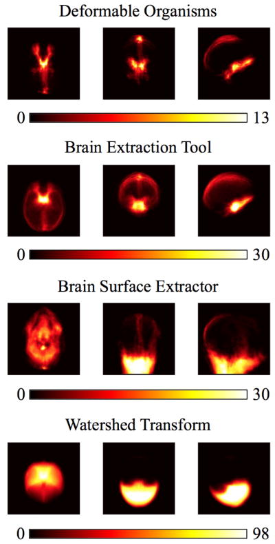
We show the projections of the false positive errors in the axial, sagittal, and coronal planes for the 630 Australian twins dataset. Our results include our deformable organisms approach, the brain extraction tool, brain surface extractor, and watershed transform.

Figure 4.

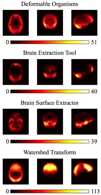
We show the projections of the false negative errors in the axial, sagittal, and coronal planes for the 630 Australian twins dataset. Our results include our deformable organisms approach, the brain extraction tool, brain surface extractor, and watershed transform.

We also list average results of deformable organisms with and without error correction versus manual training in Table 2. Random samples of 20 images from the 630 twins were selected, using 10 to train and 10 to test the error correction. We repeat this 10 times and average the results. These results were used in FDR corrected (at the 0.05 level) paired-sample t-test that found the learning step significantly improved both the Dice overlap and false negative error measures.

Table 2.

Distance, overlap, and error metrics comparing the deformable organisms segmentation with and without error correction versus manual skull-stripping in our 630 twins dataset. We show the top performing measures in bold. We carried out FDR corrected paired-sample t-tests to compare before and after the machine learning step and found significant improvements in the Dice overlap and false positive error measures. This improvement is promising because false positive error was the worst performing metric in our approach.

	Hausdorff Distance	Jaccard Overlap	Dice Overlap	False Positive Error	False Negative Error
Basic DO	35.48±2.79	0.8485±0.0009	0.9178±0.0005	0.0256±0.0006	0.1318±0.0010
DO with correction	35.52±3.13	0.8858±0.0013	0.9393±0.0007	0.0253±0.0004	0.0929±0.0012

Table 3 shows the corresponding metric values for the ADNI dataset. In this case we left out the HWA method since it was used as a step in creating the gold standard images. Because the ADNI dataset if of much older adults with many subjects having moderate to severe atrophy due to dementia, skull-stripping is relatively more challenging and the metric performance across all methods is much lower, but at the same time provides a good way to test how robust each approach is to abnormal data. We used paired-sample t-tests to compare the BSE and BET with the deformable organisms method and found that deformable organisms ranked highest in the Hausdorff distance and false positive error metrics and was not significantly different from BSE and BET in the Jaccard and Dice metrics. It did have the highest false negative error, meaning the method will leave too much from the boundary. We also corrected results here with FDR at the 0.05 level, which resulted in a significance threshold ≪ 1.0 × 10⁻⁹ for both the deformable organisms vs. BET and deformable organisms vs. BSE because of the large difference in metric results.

Table 3.

We show the Hausdorff distance and overlap metrics (Jaccard, Dice, false negative error, and false positive error) that result from the comparison of automated segmentation algorithms with manual skull-stripping using 208 subjects that include healthy elderly controls, early- and late-stage mild cognitive impaired people, and Alzheimer’s disease patients. The automated methods include our deformable organisms approach, the brain extraction tool (BET), and brain surface extractor (BSE). We did not include the watershed algorithm in this experiment because the manual segmentation were partly delineated using the watershed approach followed by manual cleanup. The top performing measures are in bold. We computed paired-sample t-tests comparing the deformable organisms approach to the other methods and corrected for multiple comparisons across the metrics using FDR. Our results showed deformable organisms had significantly better Hausdorff distance and false positive error compared to BET and BSE. In addition, the Jaccard and Dice measures were not significantly different from the performance of BET, though it did have the highest false negative error.

	Hausdorff Distance	Jaccard Overlap	Dice Overlap	False Positive Error	False Negative Error
Deformable Organisms	31.91±33.17	0.5987±0.2118	0.7191±0.2286	0.1349±0.2802	0.3399±0.2056
BET	58.82±21.45	0.6178±0.1683	0.7501±0.1328	0.3482±0.1923	0.0604±0.0344
BSE	128.18±24.65	0.3008±0.1662	0.4400±0.1797	0.6949±0.1758	0.0213±0.0166

In Figs. 5 and 6 we show the false positive and false negative errors sampled from the 208 images in the ADNI dataset. The false positive errors in the deformable organisms approach are localized in the occipital lobe and partially in the parietal lobe while for BET and BSE the majority of errors are located in the neck area. The deformable organisms method has the largest number of false negative errors located in the cerebellum and temporal lobe while BET has its errors in the superior part of the parietal lobe while the errors in BSE are collected in the anterior part of the frontal lobe.

Figure 5.

We show the projections of the false positive errors in the axial, sagittal, and coronal planes for the 208 images from the Alzheimer’s disease dataset. Our results include our deformable organisms approach, the brain extraction tool and brain surface extractor.

Figure 6.

We show the projections of the false negative errors in the axial, sagittal, and coronal planes for the 208 images from the Alzheimer’s disease dataset. Our results include our deformable organisms approach, the brain extraction tool and brain surface extractor.

Table 4 shows the results of the deformable organisms approach with and without the error correction step. It uses the same approach in the twins analysis by learning the errors on 10 images while testing it on 10 separate images and repeating the process 10 times. The results using paired-sample t-tests before and after the steps shows that when correcting for multiple comparisons using FDR at the 0.05 level, the learning step significantly improved performance across all the metrics.

Table 4.

Distance, overlap, and error metrics comparing the deformable organisms segmentation with and without error correction versus manual skull-stripping. These results are from our Alzheimer’s disease (AD) dataset that included healthy elderly controls, early- and late-stage mild cognitive impaired people, and AD patients. The correction step improved performance in all of our metrics. We show the top performing measures in bold. We carried out FDR corrected paired-sample t-tests to compare before and after the machine learning step and found significant improvements in all of the metrics.

	Hausdorff Distance	Jaccard Overlap	Dice Overlap	False Positive Error	False Negative Error
Basic DO	60.0843±41.1119	0.3787±0.2819	0.4846±0.3223	0.4298±0.3669	0.4539±0.3510
DO with correction	50.8589±31.4044	0.4925±0.3093	0.5945±0.3215	0.3777±0.2896	0.3792±0.3464

5. Discussion

The metrics in Tables 1 and 3 suggest that in general the performance of our deformable organisms approach is comparable to that of other widely used methods. It performed particularly well in the Dice overlap and false positive error meaning it avoids including too many voxels in the boundary. The deformable organism plan did not fare as well in the false negative error and as a consequence may not include enough voxels inside the brain boundary. However, we stress that our objective is to simply evaluate if our definition of deformable organisms for MRI images can be effective for segmentation, with skull-stripping being a convenient and established example.

There is also considerable variability in the validation results for skull-stripping algorithms depending on their parameter settings and the datasets used. In (Leung et al., 2011), the authors used ADNI images to train and validate their methods. In their approach they set aside a subset of the data to train the parameters of BET, BSE, and HWA and evaluated the trained methods on a separate test dataset. Their default performance of BET is similar to our results though our images come from a different set of subjects as part of the second phase of ADNI. As mentioned by Iglesias et al. (2011), the results of BSE are highly dependent on its parameters being tuned to a dataset with a significant drop in accuracy when the default parameters are used. Our goal in the current study was to evaluate whether our framework could create comparable segmentation results with the most widely used approaches. Alternative approaches could involve the authors of each method optimizing and training their methods on our test dataset (Iglesias et al., 2011) or searching the parameter space for each algorithm for their optimal performance on a separate training dataset (Leung et al., 2011), but we found in most neuroimaging studies the researchers are not using these approaches. In addition, by training the parameters of an algorithm it could be difficult to understand if the method is an accurate representation and model of the brain boundary or instead is reduced to some kind of segmentation regularization. We also acknowledge that although our deformable organisms results were similar to the other approaches in the ADNI dataset and that there is a positive correlation between segmentation error and subject age (Iglesias et al., 2011), because of the relatively low performance it could be that the method is not able to generalize as well and future work could involve modifying the plan to work with more diverse data.

Tables 2 and 4 show that learning errors improves the segmentation performance in a range of metrics depending on the dataset used. Th improvement in false negative error is promising, as it shows that the machine learning step is able to compensate for the low performance in the initial plan specification. The training step may be useful if a large data set needs to be segmented, making it reasonable to segment some images manually for error correction. The method could be trained on a small subset of the manual and automatically segmented data, in a first pass, and the error corrections learned could be useful to segment the rest of the dataset.

In our experiments we focused on a skull-stripping plan for the deformable organisms, but our framework can be used in the future for a variety of segmentation problems. The related problem of skull-stripping MRI images that have tumors (Zhao et al., 2010) could be addressed by our framework with the addition of a tumor organism that localizes the tumor boundary so it will not interfere with finding an accurate brain boundary. The behaviors and image processing we described may be adept at labeling the bones in images of the hand (Michael and Nelson, 1989), where an organism can map each bone and vary its own boundary significantly while respecting the integrity of the surrounding bone boundaries. Another use for the organisms could be a complete segmentation of the brain tissue and would need a far more detailed plan to be successful, but could be more robust than the current atlas based approaches because of the organisms’ ability to uniquely deform themselves while searching for a specified goal.

We used a machine learning algorithm to fix errors in the deformable organism plan as a final step, but it could be incorporated more extensively throughout the plan. Each organism could have its own trained model to classify its boundary voxels and improve its segmentation to the benefit of surrounding organisms. Even the deformations could be influenced by a learned global model of the most probable deformations similar to an active shape or active appearance model or incorporate information about the segmentation uncertainty (Beutner III et al., 2009). Any of these or more sophisticated statistical techniques (Shen et al., 2001; Zaidi et al., 2006) may be integrated into an organism specification or simply complement the organisms in the plan.

Our deformable organisms could have been represented as level sets (Osher and Sethian, 1988), point-set surfaces (Amenta and Kil, 2004), or graph-cuts (Amenta and Kil, 2004), but our framework has advantages for specifying detailed behaviors. We may define a behavior that vastly changes the landscape of the potential function we are optimizing without having to deal with the computationally expensive numerical solutions to level sets. Our deformable organisms have some constraints on shape and size provided by curvature weighted smoothing but other smoothing techniques such a feature-preserving statistical estimation approach (Jones et al., 2003) or a method based on adaptive and anisotropic Gaussian filters (Belyaev and Seidel, 2002) may provide more freedom to follow a boundary while preserving shape at previously recognized locations.

There are similarities between our approach and the Markov random field (MRF) based segmentation approaches (Zhang et al., 2001; Held et al., 1997). MRF methods enforce priors on the pixel intensities based on the neighborhood of intensity information. On the other hand, deformable organism is a more direct approach to finding the brain-skull boundary based on a recently developed model. It has a number of advantages: 1) Behavior of different regions can be locally controlled. 2) This model is robust to noise as shape of the brain boundary is defined by warping of the contour model. 3) Topology of the boundary can be controlled by adding appropriate constrains on the deformable model. These unique advantages of the deformable organism model make it particularly attractive for the purpose of skull extraction. For comparison, we have included methods that use MRF models (e.g. BSE and HWA).

Researchers may specify countless plans for segmentation that use our deformable organism definitions and future work could address how to properly design and optimize these plans. Thimbleby et al. (1995) introduced conventions that organisms should adhere to when they interact or cooperate, concepts also presented by Doran et al. (1997). These rules could be incorporated into the cognition layer to automatically regulate how organisms interact in a plan. In addition, we could find the best plan for segmentation by comparing the delineations from sample plans to manual segmentations, a process that may be optimized using genetic (Goldberg, 1989) or evolutionary algorithms (Zitzler and Thiele, 1999).

In the context of segmentation in medical images, our deformable organisms aspire to be a framework that researchers use to specify high-level goals and problem or data specific information to segment an image. If a user encounters data that is noisy in certain areas, that information could be used so that organisms in other areas would have precedence in fulfilling their objective and errors from the noisy areas could be contained so it does not affect the final segmentation greatly. This malleability in the application of a deformable organisms method could be valuable to connect the specialized boundaries of a manual protocol with the detailed image processing capabilities of modern algorithms.

References

- Amenta N, Kil Y. ACM Transactions on Graphics (TOG) Vol. 23. ACM; 2004. Defining point-set surfaces; pp. 264–270. [Google Scholar]
- Belyaev Y, Seidel H. Mesh smoothing by adaptive and anisotropic Gaussian filter applied to mesh normals. Vision, Modeling, and Visualization. 2002:203–210. [Google Scholar]
- Benjamini Y, Hochberg Y. Controlling the false discovery rate: a practical and powerful approach to multiple testing. Journal of the Royal Statistical Society Series B (Methodological) 1995;57(1):289–300. [Google Scholar]
- Beutner K, III, Prasad G, Fletcher E, DeCarli C, Carmichael O. Information Processing in Medical Imaging. Springer; Berlin Heidelberg: 2009. Estimating uncertainty in brain region delineations; pp. 479–490. [DOI] [PMC free article] [PubMed] [Google Scholar]
- Boesen K, Rehm K, Schaper K, Stoltzner S, Woods R, Luders E, Rottenberg D. Quantitative comparison of four brain extraction algorithms. NeuroImage. 2004;22(3):1255–1261. doi: 10.1016/j.neuroimage.2004.03.010. [DOI] [PubMed] [Google Scholar]
- Crum W, Camara O, Rueckert D, Bhatia K, Jenkinson M, Hill D. Generalised overlap measures for assessment of pairwise and groupwise image registration and segmentation. Medical Image Computing and Computer-Assisted Intervention–MICCAI 2005. 2005;8:99–106. doi: 10.1007/11566465_13. [DOI] [PubMed] [Google Scholar]
- Desbrun M, Meyer M, Schroder P, Barr A. Implicit fairing of irregular meshes using diffusion and curvature flow. Proceedings of the 26th Annual Conference on Computer Graphics and Interactive Techniques; ACM Press/Addison-Wesley Publishing Co; 1999. pp. 317–324. [Google Scholar]
- Dice L. Measures of the amount of ecologic association between species. Ecology. 1945;26(3):297–302. [Google Scholar]
- Doran J, Franklin S, Jennings N, Norman T. On cooperation in multi-agent systems. The Knowledge Engineering Review. 1997;12(3):309–314. [Google Scholar]
- Freund Y, Schapire R. Computational Learning Theory. Springer; 1995. A desicion-theoretic generalization of on-line learning and an application to boosting; pp. 23–37. [Google Scholar]
- Gelman A, Hill J. Data analysis using regression and multilevel/hierarchical models. Cambridge University Press; 2007. [Google Scholar]
- Gering D, Nabavi A, Kikinis R, Hata N, O’Donnell L, Grimson W, Jolesz F, Black P, Wells W., III An integrated visualization system for surgical planning and guidance using image fusion and an open MR. Journal of Magnetic Resonance Imaging. 2001;13(6):967–975. doi: 10.1002/jmri.1139. [DOI] [PubMed] [Google Scholar]
- Gharachorloo N, Gupta S, Sproull R, Sutherland I. A characterization of ten rasterization techniques. ACMSIGGRAPH Computer Graphics. 1989;23(3):355–368. [Google Scholar]
- Goldberg D. Genetic algorithms in search, optimization, and machine learning. Addison-Wesley Professional; 1989. [Google Scholar]
- Hamarneh G, McIntosh C. Physics-based deformable organisms for medical image analysis. Society of Photo-Optical Instrumentation Engineers (SPIE) Conference Series; 2005. pp. 326–335. [Google Scholar]
- Held K, Kops E, Krause B, Wells WI, Kikinis R, Muller-Gartner H. Markov random field segmentation of brain mr images. Medical Imaging, IEEE Transactions on. 1997;16(6):878–886. doi: 10.1109/42.650883. [DOI] [PubMed] [Google Scholar]
- Huttenlocher D, Klanderman G, Rucklidge W. Comparing images using the Hausdorff distance. IEEE Transactions on Pattern Analysis and Machine Intelligence. 1993;15:850–863. [Google Scholar]
- Ibanez L, Schroeder W, Ng L, Cates J. The ITK Software Guide. 2. Kitware, Inc; 2005. http://www.itk.org/ItkSoftwareGuide.pdf. [Google Scholar]
- Iglesias J, Liu C, Thompson P, Tu Z. Robust brain extraction across datasets and comparison with publicly available methods. Medical Imaging, IEEE Transactions on. 2011;30(9):1617–1634. doi: 10.1109/TMI.2011.2138152. [DOI] [PubMed] [Google Scholar]
- Jaccard P. The distribution of the flora in the alpine zone. New Phytologist. 1912;11(2):37–50. [Google Scholar]
- Jack C, Jr, Bernstein M, Borowski B, Gunter J, Fox N, Thompson P, Schuff N, Krueger G, Killiany R, DeCarli C, et al. Update on the magnetic resonance imaging core of the Alzheimer’s disease neuroimaging initiative. Alzheimer’s & Dementia. 2010;6(3):212–220. doi: 10.1016/j.jalz.2010.03.004. [DOI] [PMC free article] [PubMed] [Google Scholar]
- Jenkinson M, Smith S. A global optimisation method for robust affine registration of brain images. Medical Image Analysis. 2001;5(2):143–156. doi: 10.1016/s1361-8415(01)00036-6. [DOI] [PubMed] [Google Scholar]
- Jones T, Durand F, Desbrun M. ACM Transactions on Graphics (TOG) Vol. 22. ACM; 2003. Non-iterative, feature-preserving mesh smoothing; pp. 943–949. [Google Scholar]
- Joshi A, Lepore N, Joshi S, Lee A, Barysheva M, Stein J, McMahon K, Johnson K, de Zubicaray G, Martin N, et al. The contribution of genes to cortical thickness and volume. NeuroReport. 2011;22(3):101–105. doi: 10.1097/WNR.0b013e3283424c84. [DOI] [PMC free article] [PubMed] [Google Scholar]
- Klein A, Andersson J, Ardekani B, Ashburner J, Avants B, Chiang M, Christensen G, Collins D, Gee J, Hellier P, et al. Evaluation of 14 nonlinear deformation algorithms applied to human brain MRI registration. NeuroImage. 2009;46(3):786–802. doi: 10.1016/j.neuroimage.2008.12.037. [DOI] [PMC free article] [PubMed] [Google Scholar]
- Leung K, Barnes J, Modat M, Ridgway G, Bartlett J, Fox N, Ourselin S. Automated brain extraction using multi-atlas propagation and segmentation (MAPS). International Symposium on Biomedical Imaging, ISBI; 2011; IEEE; 2011. pp. 1662–1665. [Google Scholar]
- Lorensen W, Cline H. Marching cubes: A high resolution 3D surface construction algorithm. ACM Siggraph Computer Graphics. 1987;21(4):163–169. [Google Scholar]
- McInerney T, Hamarneh G, Shenton M, Terzopoulos D. Deformable organisms for automatic medical image analysis. Medical Image Analysis. 2002;6(3):251–266. doi: 10.1016/s1361-8415(02)00083-x. [DOI] [PMC free article] [PubMed] [Google Scholar]
- McInerney T, Terzopoulos D. Deformable models in medical image analysis: a survey. Medical Image Analysis. 1996;1(2):91–108. doi: 10.1016/s1361-8415(96)80007-7. [DOI] [PubMed] [Google Scholar]
- McIntosh C, Hamarneh G. I-DO: A Deformable Organisms framework for ITK. The Insight Journal; 2006 MICCAI Open Science Workshop; 2006a. pp. 1–14. [Google Scholar]
- McIntosh C, Hamarneh G. Spinal crawlers: Deformable organisms for spinal cord segmentation and analysis. Proceedings of the 9th international conference on Medical Image Computing and Computer-Assisted Intervention; Springer; 2006b. pp. 808–815. [DOI] [PubMed] [Google Scholar]
- McIntosh C, Hamarneh G. Vessel crawlers: 3D physically-based deformable organisms for vasculature segmentation and analysis. Computer Vision and Pattern Recognition, 2006 IEEE Computer Society Conference on; 2006c. pp. 1084–1091. [Google Scholar]
- McIntosh C, Hamarneh G, Mori G. Human limb delineation and joint position recovery using localized boundary models. Motion and Video Computing, 2007. WMVC’07. IEEE Workshop on; IEEE; 2007. pp. 31–31. [Google Scholar]
- Michael D, Nelson A. HANDX: A model-based system for automatic segmentation of bones from digital hand radiographs. Medical Imaging, IEEE Transactions on. 1989;8(1):64–69. doi: 10.1109/42.20363. [DOI] [PubMed] [Google Scholar]
- Nir T, Jahanshad N, Villalon-Reina J, Toga A, Jack C, Weiner M, Thompson P. Effectiveness of regional DTI measures in distinguishing Alzheimer’s disease, MCI, and normal aging. NeuroImage: clinical. 2013;3:180–195. doi: 10.1016/j.nicl.2013.07.006. [DOI] [PMC free article] [PubMed] [Google Scholar]
- Ohtake Y, Belyaev A, Bogaevski I. Polyhedral surface smoothing with simultaneous mesh regularization. Geometric Modeling and Processing 2000; Theory and Applications. Proceedings; IEEE; 2002. pp. 229–237. [Google Scholar]
- Osher S, Sethian J. Fronts propagating with curvature-dependent speed: algorithms based on Hamilton-Jacobi formulations. Journal of Computational Physics. 1988;79(1):12–49. [Google Scholar]
- Pineda J. A parallel algorithm for polygon rasterization. ACM SIGGRAPH Computer Graphics. 1988;22(4):17–20. [Google Scholar]
- Prasad G, Joshi A, Thompson P, Toga A, Shattuck D, Terzopoulos D. Skull-stripping with deformable organisms. Biomedical Imaging: From Nano to Macro, 2011 IEEE International Symposium on; IEEE; 2011a. pp. 1662–1665. [DOI] [PMC free article] [PubMed] [Google Scholar]
- Prasad G, Joshi AA, Feng A, Barysheva M, Mcmahon KL, De Zubicaray GI, Martin NG, Wright MJ, Toga AW, Terzopoulos D, et al. Deformable organisms and error learning for brain segmentation. Proceedings of the Third International Workshop on Mathematical Foundations of Computational Anatomy-Geometrical and Statistical Methods for Modelling Biological Shape Variability; 2011b. pp. 135–147. [Google Scholar]
- Prasad G, Joshi S, Jahanshad N, Villalon J, Aganj I, Lenglet C, Sapiro G, McMahon K, de Zubicaray G, Martin N, Wright M, Toga A, Thompson P. White matter tract analysis in 454 adults using maximum density paths. Medical Image Computing and Computer-Assisted Intervention Workshop on Computational Diffusion MRI; 2011c. pp. 1–12. [Google Scholar]
- Prasad G, Joshi S, Jahanshad N, Villalon-Reina J, Aganj I, Lenglet C, Sapiro G, McMahon K, de Zu-bicaray G, Martin N, et al. Automatic clustering and population analysis of white matter tracts using maximum density paths. NeuroImage. 2014 doi: 10.1016/j.neuroimage.2014.04.033. [DOI] [PMC free article] [PubMed] [Google Scholar]
- Resnick S, Pham D, Kraut M, Zonderman A, Davatzikos C. Longitudinal magnetic resonance imaging studies of older adults: a shrinking brain. Journal of Neuroscience. 2003;23(8):3295–3301. doi: 10.1523/JNEUROSCI.23-08-03295.2003. [DOI] [PMC free article] [PubMed] [Google Scholar]
- Roche A, Malandain G, Pennec X, Ayache N. The correlation ratio as a new similarity measure for multimodal image registration. Medical Image Computing and Computer-Assisted Interventation–MICCAI 1998. 1998;1:1115–1124. [Google Scholar]
- Segonne F, Dale A, Busa E, Glessner M, Salat D, Hahn H, Fischl B. A hybrid approach to the skull stripping problem in MRI. NeuroImage. 2004;22(3):1060–1075. doi: 10.1016/j.neuroimage.2004.03.032. [DOI] [PubMed] [Google Scholar]
- Shattuck D, Leahy R. BrainSuite: an automated cortical surface identification tool. Medical Image Analysis. 2002;6(2):129–142. doi: 10.1016/s1361-8415(02)00054-3. [DOI] [PubMed] [Google Scholar]
- Shattuck D, Mirza M, Adisetiyo V, Hojatkashani C, Salamon G, Narr K, Poldrack R, Bilder R, Toga A. Construction of a 3D probabilistic atlas of human cortical structures. NeuroImage. 2008;39(3):1064–1080. doi: 10.1016/j.neuroimage.2007.09.031. [DOI] [PMC free article] [PubMed] [Google Scholar]
- Shattuck D, Prasad G, Mirza M, Narr K, Toga A. Online resource for validation of brain segmentation methods. NeuroImage. 2009;45(2):431–439. doi: 10.1016/j.neuroimage.2008.10.066. [DOI] [PMC free article] [PubMed] [Google Scholar]
- Shen D, Herskovits E, Davatzikos C. An adaptive-focus statistical shape model for segmentation and shape modeling of 3-D brain structures. Medical Imaging, IEEE Transactions on. 2001;20(4):257–270. doi: 10.1109/42.921475. [DOI] [PubMed] [Google Scholar]
- Smith S. Fast robust automated brain extraction. Human Brain Mapping. 2002;17(3):143–155. doi: 10.1002/hbm.10062. [DOI] [PMC free article] [PubMed] [Google Scholar]
- Steels L. The artificial life roots of artificial intelligence. Artificial Life. 1993;1(1–2):75–110. [Google Scholar]
- Terzopoulos D, Platt J, Barr A, Fleischer K. Elastically deformable models. ACM Siggraph Computer Graphics. 1987;21(4):205–214. [Google Scholar]
- Thimbleby H, Witten I, Pullinger D. Concepts of cooperation in artificial life. Systems, Man and Cybernetics, IEEE Transactions on. 1995;25(7):1166–1171. [Google Scholar]
- Thompson P, Cannon T, Narr K, Van Erp T, Poutanen V, Huttunen M, Lönnqvist J, Standertskjöld-Nordenstam C, Kaprio J, Khaledy M, et al. Genetic influences on brain structure. Nature Neuroscience. 2001;4(12):1253–1258. doi: 10.1038/nn758. [DOI] [PubMed] [Google Scholar]
- Thompson P, Hayashi K, De Zubicaray G, Janke A, Rose S, Semple J, Herman D, Hong M, Dittmer S, Doddrell D, et al. Dynamics of gray matter loss in Alzheimer’s disease. Journal of Neuroscience. 2003;23(3):994–1005. doi: 10.1523/JNEUROSCI.23-03-00994.2003. [DOI] [PMC free article] [PubMed] [Google Scholar]
- Thompson P, Hayashi K, Sowell E, Gogtay N, Giedd J, Rapoport J, De Zubicaray G, Janke A, Rose S, Semple J, et al. Mapping cortical change in Alzheimer’s disease, brain development, and schizophrenia. NeuroImage. 2004;23:S2–S18. doi: 10.1016/j.neuroimage.2004.07.071. [DOI] [PubMed] [Google Scholar]
- Wang H, Das S, Suh J, Altinay M, Pluta J, Craige C, Avants B, Yushkevich P. A learning-based wrapper method to correct systematic errors in automatic image segmentation: Consistently improved performance in hippocampus, cortex and brain segmentation. NeuroImage. 2011;55(3):968–985. doi: 10.1016/j.neuroimage.2011.01.006. [DOI] [PMC free article] [PubMed] [Google Scholar]
- Woods R, Dapretto M, Sicotte N, Toga A, Mazziotta J. Creation and use of a Talairach-compatible atlas for accurate, automated, nonlinear intersubject registration, and analysis of functional imaging data. Human Brain Mapping. 1999;8(2–3):73–79. doi: 10.1002/(SICI)1097-0193(1999)8:2/3<73::AID-HBM1>3.0.CO;2-7. [DOI] [PMC free article] [PubMed] [Google Scholar]
- Zaidi H, Ruest T, Schoenahl F, Montandon M, et al. Comparative assessment of statistical brain MR image segmentation algorithms and their impact on partial volume correction in PET. Neuroimage. 2006;32(4):1591–1607. doi: 10.1016/j.neuroimage.2006.05.031. [DOI] [PubMed] [Google Scholar]
- Zhang Y, Brady M, Smith S. Segmentation of brain mr images through a hidden markov random field model and the expectation-maximization algorithm. Medical Imaging, IEEE Transactions on. 2001;20(1):45–57. doi: 10.1109/42.906424. [DOI] [PubMed] [Google Scholar]
- Zhao W, Xie M, Gao J, Li T. A modified skull-stripping method based on morphological processing. Computer Modeling and Simulation, 2010. ICCMS’10. Second International Conference on; IEEE; 2010. pp. 159–163. [Google Scholar]
- Zitzler E, Thiele L. Multiobjective evolutionary algorithms: A comparative case study and the strength pareto approach. Evolutionary Computation, IEEE Transactions on. 1999;3(4):257–271. [Google Scholar]