Distinguishing State Variability From Trait Change in Longitudinal Data: The Role of Measurement (Non)Invariance in Latent State-Trait Analyses

Abstract

Researchers analyzing longitudinal data often want to find out whether the process they study is characterized by (1) short-term state variability, (2) long-term trait change, or (3) a combination of state variability and trait change. Classical latent state-trait (LST) models are designed to measure reversible state variability around a fixed set-point or trait, whereas latent growth curve (LGC) models focus on long-lasting and often irreversible trait changes. In the present paper, we contrast LST and LGC models from the perspective of measurement invariance (MI) testing. We show that establishing a pure state-variability process requires (a) the inclusion of a mean structure and (b) establishing strong factorial invariance in LST analyses. Analytical derivations and simulations demonstrate that LST models with non-invariant parameters can mask the fact that a trait-change or hybrid process has generated the data. Furthermore, the inappropriate application of LST models to trait change or hybrid data can lead to bias in the estimates of consistency and occasion-specificity, which are typically of key interest in LST analyses. Four tips for the proper application of LST models are provided.

A growing body of research in psychology and the social sciences is concerned with the analysis of the longitudinal dynamics of psychological and social science constructs. This can be seen from (1) the increasing number of substantive studies that present data from at least two measurement occasions and (2) the large body of methodological literature dealing with the development, presentation, evaluation, and refinement of statistical methods for analyzing longitudinal data (e.g., Bollen & Curran, 2006; Chan, 1998; Collins & Sayer, 2001; Duncan, Duncan, & Strycker, 2006; Eid, 2007; McArdle, 2009). As explained below, in the analysis of the longitudinal dynamics of psychological phenomena, an important distinction can be made between state variability processes on the one hand and trait-change processes on the other hand.

Modeling State Variability Versus Trait Change

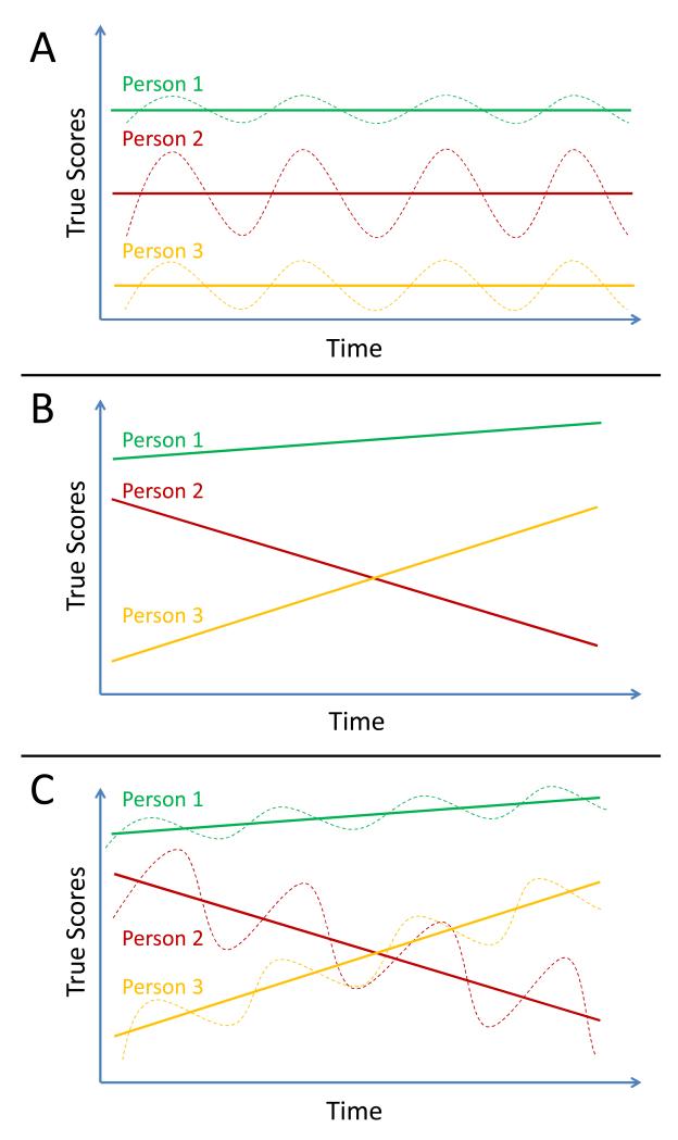
In line with Nesselroade (1991), we refer to state variability as a process that involves reversible short-term changes in individuals’ true scores around an invariant set-point or trait value and to trait change as a process that involves long-lasting and potentially irreversible modifications of psychological traits. Whereas trait change involves changes in the trait values themselves, state variability implies that individuals’ trait values do not change, but that there are systematic time- or situation-specific “ups and downs” in individuals’ true state scores around the fixed trait. Figure 1A illustrates a hypothetical state-variability process for three individuals. It can be seen that although inter-individual differences in the trait scores (indicated by the solid lines) are present, there are no intra-individual changes in the trait scores across time. The longitudinal process is characterized by intra-individually stable trait values plus momentary (situation-specific) deviations (indicated by the dotted lines) of the true scores from the stable trait values.

Figure 1.

Illustration of different types of longitudinal processes for three hypothetical individuals. Solid lines show the trait scores. Dotted lines show systematic situation-specific deviations of the latent state scores from the trait scores (state variability). A: Pure state-variability process. B: Pure trait-change process. C: Hybrid case including both a state-variability and a trait-change process.

As an example of a state-variability process, consider mood states. The longitudinal course of many mood constructs can be described by a stable trait mood level with momentary deviations from this trait (Eid, Schneider, & Schwenkmezger, 1999). Although systematic intra-individual variations in state mood levels across time are expected, these differences represent state variability (ups and downs) around a fixed set-point for most people rather than enduring changes or “growth” in people’s trait mood. (Note that state variability is distinct from measurement error, which represents a separate, unsystematic source of variability as shown below.)

Figure 1B illustrates a pure trait-change process. It can be seen that individuals’ trait scores change linearly across time in this example. There are no situation-specific deviations from the growth trajectory. As an example of a pure trait-change process, consider the development of height in children, which involves enduring changes in body length that follow a certain trajectory and are irreversible, at least until late adulthood. Situation-specific deviations from the general growth trajectory would be unlikely in this example, given that physical growth typically does not show situation-specific ups and downs that can be expected for many psychological variables.

Figure 1C shows a hybrid case, in which the longitudinal process involves both a state-variability component and a trait-change component. As an example, consider depressed patients who undergo psychotherapy. Despite the fact that, as a result of the therapy, the patients show long-term changes (declines) in their depression trait levels, there will likely still be days on which the patients feel better or worse relative to the general decline trajectory. We suspect that hybrid cases as the one shown in Figure 1C may be common in psychological research, as many constructs have both trait and state components (e.g., Hertzog & Nesselroade, 1987) and at the same time may involve enduring changes to the trait scores across time.

State variability (reversible short-term change) and trait (irreversible long-term) change are conceptually and empirically distinct psychological processes. In longitudinal applications, it is usually of interest to researchers which process generated the data. For example, in intervention studies, it is relevant whether changes seen in true scores after, for example, psychotherapy reflect merely short-term variability or whether they are indicative of a long-term trait modification.

The different longitudinal processes described above are reflected in different types of statistical models for longitudinal data. Whereas models of latent state-trait (LST) theory (Steyer, Majcen, Schwenkmezger, & Buchner, 1989; Steyer, Ferring, & Schmitt, 1992; Steyer, Schmitt, & Eid, 1999) represent prototypical models for measuring state-variability processes, trait change (or growth trajectory) processes are often assessed with latent growth curve (LGC; Meredith & Tisak, 1990; McArdle, 1988) or latent (trait) change score models (McArdle & Hamagami, 2001; Raykov, 1993; Steyer, Eid, & Schwenkmezger, 1997). Hybrid models (e.g., Eid & Hoffmann, 1998; Tisak & Tisak, 2000) combine features of both, models of state-variability and models of trait change.

In this article, we are concerned with the role that longitudinal measurement invariance (MI) plays in distinguishing short-term state-variability processes from long-term trait-change (or growth trajectory) processes. The purpose of this article is to show that researchers’ ability to discriminate between state-variability and trait-change processes depends crucially on whether they employ tests of MI not only in trait-change (e.g., LGC) models, but also in state-variability models (i.e., classical LST models). Whereas researchers routinely test for MI in trait-change models, testing MI has been widely neglected in past applications of LST models as we demonstrate later in this article. We show that when certain measurement parameters are non-invariant in an LST model, this may indicate that a trait-change process rather than (or in addition to) a state-variability (state-trait) process should be modeled. In other words, measurement non-invariance in LST models can mask true trait changes (or growth processes) in the underlying construct.

In our presentation, we contrast two prototypical models against each other: (1) the singletrait-multistate (STMS) model as a classical LST model for measuring short-term state-variability processes and (2) a multiple-indicator linear LGC model that can be seen as a hybrid model, capturing both long-term trait-change processes and short-term state-variability processes. We first show analytically which consequences may arise from measurement non-invariance in LST models. Second, we introduce a hybrid model and illustrate through a simulation study that LST models with non-invariant parameters can fit data generated by a trait-change (growth) process well and lead to bias in the estimation of variance components.

In the following section, we provide a non-technical review of LGC and LST models as well as the concept of MI before providing the formal details on why it is important to test for MI not only in models of trait change, but also in LST models of state-variability processes. For didactic reasons, we begin our review with LGC models, for which the requirement of MI—as well as the consequences of non-invariance—are widely accepted in the literature.

Latent Growth Curve (LGC) Models

Standard LGC models are appropriate models when the underlying longitudinal process is best described as a long-lasting trait-change process such as, for example, a process of enduring changes in height, intelligence, or skills (see Figure 1B). LGC models are also referred to as growth trajectory models, because they focus on more enduring trait-change processes. These models typically include a continuous latent factor that represents true individual differences in people’s trait scores at a particular time point (often the first time point) and is called intercept factor. In addition, LGC models usually feature one or more continuous latent factors that represent individual differences in the rate of trait change over time, the so-called latent slope, shape, or curve factors. Depending on the hypotheses of a researcher, the slope factor(s) can represent, for example, linear, quadratic, cubic, or an unspecified form of change. In LGC models, the focus is typically on the separation of measurement error from true individual differences in initial status and trait change as well as on the estimation of the “growth parameters”, such as means, variances, and covariances of intercept and slope factors. In addition, covariates or outcomes of trait change may also be included in the model.

MI in models of trait change

One important aspect to the measurement of trait changes that has been widely recognized in the literature is the requirement that psychological traits be measured on the same scale (i.e., with the same origin and units of measurement) at each time point so that meaningful across-time comparisons can be made. This issue is known as the problem of MI (e.g., Borsboom, 2006; Chan, 1998; Cheung & Rensvold, 1999; Meredith, 1993; Millsap, 2011; Vandenberg & Lance, 2000; Widaman & Reise, 1997). In longitudinal studies, MI refers to whether the parameters of the measurement model (i.e., the factor loadings, measurement intercepts, and measurement error variances) that relate an observed variable (indicator) to a latent variable have the same value at each measurement occasion. For most types of longitudinal CFA models including LGC models (e.g., Chan, 1998; Ferrer, Baluerka, & Widaman, 2008) and latent change models (McArdle & Hamagami, 2001; Raykov, 1993; Steyer, Eid, & Schwenkmezger, 1997), methodologists agree that MI be established before latent variable change can be meaningfully interpreted. This can be viewed as an apples-and-oranges problem. If the origin or the units of measurement change, examining mean changes in the latent variables across time can be difficult (e.g., Vandenberg & Lance, 2000). Ostensible differences in the latent means could just reflect changes in scale difficulty, scale discrimination, or scale meaning.

For LGC and other models of change, clear guidelines exist as to (1) how different levels of MI can be defined (Millsap & Meredith, 2007; Cheung & Rensvold, 1999; Widaman & Reise, 1997) and (2) which level of MI is necessary for a meaningful interpretation of latent change over time in these models. Widaman and Reise (1997) distinguished four levels of MI. Configural invariance only requires the number of factors and the loading pattern to be constant across time, without the necessity that specific measurement parameters be identical across time. Weak factorial invariance (also referred to as metric invariance) requires only the factor loadings to be invariant across time, whereas strong factorial invariance (or scalar invariance) requires both invariant factor loadings and intercepts. Strict factorial invariance in addition requires time-invariant measurement error variances. Strong factorial invariance is the minimum level of MI that allows for a meaningful interpretation of change in latent change and LGC models (e.g., Baumgartner & Steenkamp, 2006). Conceptually, this can be explained by the fact that time-invariant loadings and intercepts ensure that the origin and the units of measurement do not change across occasions of measurement. If strong invariance holds, the latent variables are measured on the same scale at each point in time and scores on the latent variables can be meaningfully compared across time.

In practice, MI is often tested in terms of absolute model fit or by comparing the relative model fit of competing invariance models (e.g., the configural, weak, strong, and strict factorial invariance models; Cheung & Rensvold, 2002). The most parsimonious model that still shows an adequate fit is usually retained. Researchers typically hope that they can retain a model that has a sufficient level of MI for the purposes of the study—often a model that postulates at least strong factorial invariance. If strong factorial invariance cannot be established for all indicators of a latent variable, a model of partial measurement invariance may still allow for a meaningful interpretation of changes across time under certain circumstances (Cheung & Rensvold, 1999).

LST Models

In contrast to LGC models, classical LST models do not focus on enduring trait changes or latent growth trajectories, but rather on short-term state-variability processes around an invariant trait and the impact of situations on psychological measurement. The basic rationale for the development of LST theory was that virtually all measurements in psychology are affected not only by random measurement error but also by systematic situation-specific influences and person × situation interactions (Anastasi, 1983; Hertzog & Nesselroade, 1987; Steyer et al., 1989; 1992; 1999). This is true even for the measurement of constructs that in theory are conceived of as stable traits (Deinzer et al., 1995).

LST models are useful, because the longitudinal course of psychological constructs cannot always be appropriately described with LGC or other types of trait-change models. As noted above, psychological constructs may be characterized by a longitudinal process of trait stability (no changes in the trait values over time) combined with short-term changes in the true states that may be due to systematic situational influences or person × situation interactions (i.e., not just measurement error). Such situation-dependent “ups and downs” would not be appropriately captured by a growth trajectory (LGC) model, but instead require an LST model. Variability models (such as LST models) are of also interest as “null hypothesis” models of no trait change, for example, in developmental psychology (no development) or clinical psychology (no enduring symptom change). As we discuss in more details later, LST models can be seen as LGC models, in which the growth factors have a mean and variance of zero (Tisak & Tisak, 2000). In summary, LST models focus on a different type of change process than LGC models: Whereas standard LGC models focus on long-term trait changes, LST models allow researchers to model short-term variability processes around an invariant trait.

As we show in more formal detail below, LST models decompose an observed score into a component that characterizes the person effect (the latent trait component that is assumed to be stable across time), a component that characterizes systematic state variability (the latent state residual component that reflects effects of the situation and person × situation interactions), and a random measurement error component (that reflects unsystematic measurement error or unreliability of the observed scores). In contrast to models designed to measure trait-change processes (such as LGC models), standard LST models used in the literature assume that there is systematic variability around the latent trait, but that the trait itself is stable and does not change over time—at least not over the course of the study from which the data were obtained¹. As such, LST models are models of state variability that are designed to identify reliable, albeit short-term and potentially reversible situation-specific fluctuations around an invariant trait as opposed to processes that involve only perfectly stable traits or processes that involve more long-lasting and potentially irreversible trait changes or growth over time (Eid, 2007).

As an example, Luhmann, Schimmack, and Eid (2011) used LST models to examine the variability and stability of subjective well-being (SWB) by parsing variance attributable to stable (trait) influences, variable state influences, and random measurement error. Seen within the LST framework, the part of SWB that represents the “set point” does not change over time. Luhmann et al. found that about 34-47% of the variability in SWB reflected stable individual differences (i.e., trait effects), whereas about 48-54% were due to a state-variability component (situation or person × situation interaction effects).

Like LGC models, measurement models derived from LST theory can be estimated in the framework of longitudinal confirmatory factor analysis (CFA). Different kinds of LST models have been discussed by Cole (2012), Eid (1996), Eid et al. (1999), Geiser and Lockhart (2012), Kenny (2001), and Steyer et al. (1992, 1999; Steyer, Geiser, & Fiege, 2012). For a comprehensive overview of LST applications in psychology and the social sciences, see Geiser and Lockhart (2012).

Measurement invariance (MI) in LST models

Even though the issue of MI has been discussed in detail for CFA models of change including LGC models (e.g., Chan, 1998), the role that MI plays in LST models has not been clarified in the literature. Moreover, a review of the LST literature since 1989 revealed that MI is rarely explicitly tested in applications of LST models. We identified 52 articles that reported applications of LST models. Only 7 applications (14%) explicitly addressed MI and used at least one strategy to test it. These studies have generally followed a model-building procedure, testing the invariance of factor loadings (e.g., Eid & Diener, 2004; Hermes et al., 2009) and indicator residual variances over time (e.g. Boll et al., 2010; Schmitt & Steyer, 1993). Many LST studies (48%) imposed the assumption of equal factor loadings, but did not evaluate model fit without this restriction. In addition, many of these studies indicated that these constraints were implemented merely for convenience to reduce parameters or to facilitate the calculation of variance components. We found five studies (9.6%) that did not impose any kind of equality constraints on parameters of the measurement model and an additional six studies (11.5%) for which the specification was unclear from the description in the papers.

Even though several methodological papers discussed MI in the context of LST models (Alessandri, Caprara, & Tisak, 2012; Baumgartner & Steenkamp, 2006; Ciesla, Cole, & Steiger, 2007; Tisak & Tisak, 2000), most methodological work in this area has not explicitly addressed whether MI is at all relevant to LST analyses and what the consequences of measurement non-invariance might be. Although Baumgartner and Steenkamp (2006) advocated a model-building procedure for establishing MI based on the item loadings and intercepts, in which loadings and intercepts are systematically released from invariance (see also Alessandri et al., 2012), they did not specifically discuss the relevance of these issues to LST analyses or for the separation of state-variability from trait-change processes.

Researchers using LST models are confronted with two key questions: First, do I need to establish MI in LST analyses before I can claim that the longitudinal process under study is best described as a short-term state-variability process and meaningfully interpret the parameters of an LST model? Second, what are the potential consequences of ignoring MI and estimating an LST model in which the measurement parameters are not invariant across time? Here, we focus in particular on the potential consequences of measurement non-invariance may have on a researcher’s ability to distinguish between a short-term state-variability versus a long-term trait-change process.

In the following section, we introduce the basic concepts of LST theory. Subsequently, we present the STMS model as a prototypical LST model. We then discuss the latent mean and variance structures in the model and implications of measurement (non)invariance across time in LST analyses for the model-implied mean and variance structure. Even though more complex LST models are often used in practice (for an overview, see Geiser & Lockhart, 2012), the key issues described here apply to more complex LST models as well.

Basic Concepts and Models of LST Theory

The starting point for an LST analysis is a set of multiple repeatedly-administered observed variables Y_it (i = indicator, i = 1,…, m; t = time point, t = 1, …, n) that pertain to the same construct (e.g., anxiety, subjective well-being, extraversion etc.). Indicators for a construct in an LST model could, for example, be different items, scale scores, or physiological measures. Similar to classical test theory, in LST theory each indicator variable is decomposed into its own (indicator-specific) latent state variable τ_it and measurement error variable ε_it:

$$Y_{it}={\tau }_{it}+{\epsilon }_{it}.$$ (1)

In LST theory, a latent state variable is defined as the conditional expectation of an observed variable given a person (or observational unit) variable U and a situation variable S_t: τ_it ≡ E(Y_it | U, S_t). This shows that the latent state variable characterizes both persons and situations, taking into account that a psychological score is never obtained in a situational vacuum (Steyer et al., 1992).

According to LST theory, each latent state variable can be decomposed into an indicator-specific latent trait variable ξ_it and an indicator-specific latent state residual variable ζ_it:

$${\tau }_{it}={\xi }_{it}+{\zeta }_{it},$$ (2)

where ξ_it ≡ E(Y_it | U) and ζ_it ≡ τ_it − ζ_it. Therefore, the trait variables ξ_it characterize person-specific (trait) effects only, whereas the latent state residual variables ζ_it characterize systematic effects of the situation or person × situation interactions (Steyer et al., 1992). State residuals thus capture the state-variability component of behavior (as opposed to trait change).

The STMS model

A simple, testable LST model can be formulated by assuming that all indicators share the same latent trait within scaling differences (assumption of congeneric latent trait variables). This assumption implies that all latent trait variables are unidimensional, so that they can be replaced by a single (“general”) latent trait factor ξ²:

$${\xi }_{it}={\alpha }_{it}+{\lambda }_{it}\xi .$$ (3)

In Equation 3, the real constants α_it and λ_it can be interpreted as intercept and factor loading parameters, respectively. Furthermore, in the STMS model, it is assumed that all indicators that are measured at the same measurement occasion share the same latent state residual factor within scaling differences (assumption of occasion-specific congenerity of latent state residuals). This implies that all latent state residual variables at the same measurement occasion are unidimensional and can be replaced by a common (occasion-specific) latent state residual factor ζ_t:

$${\zeta }_{it}={\delta }_{it}{\zeta }_t.$$ (4)

The real constant δ_it in Equation 4 can be interpreted as a factor loading parameter. Equation 4 has no additive constant, because the latent state residual variables have means of zero by definition [i.e., E(ζ_it) = E(ξ_t) = 0; Steyer et al., 1992]. In addition, the following restrictions apply in the STMS model³: E(ε_it) = Cov(ξ, ζ_t) = Cov(ξ, ε_it) = Cov(ε_it, ζ_t′) = 0, Cov(ξ_t, ζ_t′) = 0 for t ≠ t′, and Cov(ε_it, ε_i′t′) = 0 for (i, t) ≠ (i′, t′).

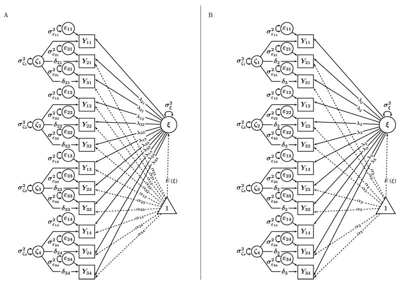
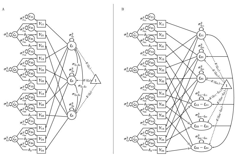
Figure 2 shows a path diagram of the STMS model for three indicators (i = 1, 2, 3) measured on three time points (t = 1, 2, 3). In this model, each observed variable measures a common, occasion-unspecific latent trait factor ξ and a common, occasion-specific latent state residual factor ζ_t. This can also be seen by inserting Equations 2, 3, and 4 into Equation 1 which yields:

$$\begin{array}{cc}\hfill Y_{it}& ={\tau }_{it}+{\epsilon }_{it}\hfill \\ \hfill & ={\xi }_{it}+{\zeta }_{it}+{\epsilon }_{it}\hfill \\ \hfill & ={\alpha }_{it}+{\lambda }_{it}\xi +{\delta }_{it}{\zeta }_t+{\epsilon }_{it}.\hfill \end{array}$$ (5)

For reasons of identification, one intercept and one loading parameter have been fixed for each factor in Figure 2. We explain these restrictions in detail below.

Figure 2.

Path diagrams illustrating the STMS model for a measurement design with three indicators and four time points. Y_it denotes the ith observed variable (indicator) measured at time t. ξ: common latent trait factor. ζ_t: latent state residual factor. α_it: constant measurement intercept. λ_it: latent trait factor loading. δ_it: latent state residual factor loading. The triangle denotes a constant of 1 that represents the mean structure in the model. The intercepts for the first indicator are set to zero (α₁ = 0) for identification and not explicitly shown in the figure. Loadings without a label are fixed to 1. A: Specification with non-invariant intercepts and factor loadings. B: Recommended specification with time-invariant intercepts and factor loadings.

The STMS model has been used, for example, by Ploubidis and Frangou (2011) to determine the proportions of variance in psychological distress attributable to state effects across two time points, representing the environmentally-induced (i.e. person-situation interaction) portion of the construct, and the effect of a single trait, representing the portion that is specific to the individual.

An important feature of LST models is the additive variance decomposition of the observed variables that follows from the fact that the latent trait, latent state residual, and measurement error variables are uncorrelated:

$$Var\left(Y_{it}\right)={\lambda }_{it}^{2}Var\left(\xi \right)+{\delta }_{it}^{2}Var\left({\zeta }_t\right)+Var\left({\epsilon }_{it}\right).$$ (6)

This additive variance decomposition allows us to compute three coefficients of determination that are of key interest to virtually all applications that have used LST models: the consistency (CO), occasion-specificity (OS), and reliability (Rel) coefficients (Steyer et al., 1999). CO indicates the degree to which individual differences on the observed variables are determined by stable person-specific (trait) effects:

$$CO\left(Y_{it}\right)=\frac{{\lambda }_{it}^{2}Var\left(\xi \right)}{Var\left(Y_{it}\right)}.$$ (7)

The CO coefficient is useful to quantify the degree of stability across situations: The larger the CO coefficient, the less the scores vary over specific situations or time points.

The OS coefficient indicates the degree to which individual differences on the observed variables are determined by the situation or person × situation interactions:

$$OS\left(Y_{it}\right)=\frac{{\delta }_{it}^{2}Var\left({\zeta }_t\right)}{Var\left(Y_{it}\right)}.$$ (8)

The OS coefficient is thus useful to quantify the extent to which the longitudinal course of a construct is affected by a state variability process: The larger the OS coefficient, the stronger the situation-specific or person × situation interaction influences on the observed scores.

The reliability coefficient indicates the degree to which observed individual differences are due to reliable sources of variances (not measurement error). Reliability equals the sum of consistency and occasion-specificity coefficient:

$$Rel\left(Y_{it}\right)=\frac{{\lambda }_{it}^{2}Var\left(\xi \right)+{\delta }_{it}^{2}Var\left({\zeta }_t\right)}{Var\left(Y_{it}\right)}=1-\frac{Var\left({\epsilon }_{it}\right)}{Var\left(Y_{it}\right)}=OS\left(Y_{it}\right)+CO\left(Y_{it}\right).$$ (9)

The consistency, occasion-specificity, and (1 – reliability) coefficients sum up to 1; that is, CO(Y_it) + OS(Y_it) + [1 − Rel(Y_it)] = 1.

In summary, the CO, OS, and Rel coefficients are often used to quantify the extent to which measurements reflect (1) stable person-specific effects (“traits”), (2) occasion-specific fluctuations (situation or person × situation interaction effects), and (3) random measurement error. For example, Kertes and van Dulmen (2012) found that cortisol levels in children showed both, substantial consistency (accounting for 43% of the variability in cortisol levels) and substantial occasion-specificity (accounting for 40% of the variance). Note that we presented the CO, OS, and Rel coefficients only for the STMS model, but that similar coefficients can be defined for other LST models as well (see Geiser & Lockhart [2012] for a detailed overview).

Mean structure

The only latent variables that can have non-zero means in LST models are the latent state variables τ_it and the latent trait variables ξ_it (as well as the corresponding common latent state and latent trait factors, which are defined on the basis of τ_it and/or ξ_it). This is because both ζ_it and ε_it are defined as regression residual variables in LST theory (Steyer et al., 1992), and regression residuals have means of zero by definition (Steyer, 1989). Hence,

$$E\left(Y_{it}\right)=E\left({\tau }_{it}\right)=E\left({\xi }_{it}\right)$$ (16)

holds for the expectation E(.) of each manifest variable Y_it. Furthermore, in the STMS model, the mean of a latent trait variable ξ_it is given by:

$$\begin{array}{cc}\hfill E\left({\xi }_{it}\right)& =E\left({\alpha }_{it}\right)+E\left({\lambda }_{it}\xi \right)\hfill \\ \hfill & ={\alpha }_{it}+{\lambda }_{it}E\left(\xi \right).\hfill \end{array}$$ (17)

Therefore, the means of the observed variables can be expressed as:

$$\begin{array}{cc}\hfill E\left(Y_{it}\right)& =E\left({\alpha }_{it}\right)+E\left({\lambda }_{it}\xi \right)+E\left({\delta }_{it}{\zeta }_t\right)+E\left({\epsilon }_{it}\right)\hfill \\ \hfill & ={\alpha }_{it}+{\lambda }_{it}E\left(\xi \right).\hfill \end{array}$$ (18)

Equation 18 shows that in LST models, the mean of each indicator depends on the mean of the corresponding latent trait factor, E(ξ), the factor loading λ_it, and the intercept parameter α_it. As a consequence, E(ξ) can be identified by setting the intercept parameter of a reference indicator (e.g., the first indicator at the first occasion of measurement) to a real value (e.g., α₁₁ = 0) and the trait factor loading of the same indicator to a positive real value (e.g., λ₁₁ = 1).

Variance structure

In the STMS model, the variances of the (indicator-specific) latent trait variables and latent state residual variables from the basic LST decomposition are given by:

$$Var\left({\xi }_{it}\right)={\lambda }_{it}^{2}Var\left(\xi \right)$$ (19)

$$Var\left({\zeta }_{it}\right)={\delta }_{it}^{2}Var\left({\zeta }_t\right).$$ (20)

Equations 19-20 show that changes in the factor loadings over time lead to changes in the variances of the (indicator-specific) latent trait and latent state residual variances in the STMS model.

MI in LST Models

One reason why the issue of MI has not yet received much explicit attention in LST modeling may be that in LST analyses the focus is on state variability rather than trait change over time. That is, researchers applying LST models typically ask whether the constructs that they study are more state-like or more trait-like (e.g., Deinzer et al., 1995; Windle & Dumenci, 1998). They focus on the proportions of the observed individual differences that are due to (1) stable person-specific effects (CO), (2) situation-specific fluctuations or person × situation interactions (OS), and (3) random error (1 − Rel). As we noted above, LST studies often assume that the trait itself does not change over the course of the study. As a consequence, LST researchers may presume that testing MI is not a critical step. Given that trait change is not explicitly modeled, no apples-and-oranges problems seem to arise. Related to this issue, researchers rarely model (or report) mean structures in LST analyses (for exceptions, see Baumgartner & Steenkamp, 2006; Alessandri et al., 2012; Lorber & O’Leary, 2012). Consequently, researchers may not even test for mean changes over time.

Because investigators using LST models are usually interested in modeling state-variability processes, they often focus exclusively on the covariance structure and on the calculation of the CO, OS, and Rel coefficients. In practice, these coefficients can be calculated even when MI is not assumed or when mean changes are present. Although this is not a problem per se, ignoring the mean structure or specifying an LST model with non-invariant parameters can obscure whether or not the trait under study actually changes across time. Furthermore, if trait change is ignored, a researcher may obtain biased estimates of the trait and state-variability related parameters of the LST model. Such bias may go unnoticed, given that LST models with non-invariant parameters may fit trait-change data very well—as we demonstrate in a simulation study below. To understand this problem, we first examine how the STMS model formally accounts for the observed and latent trait means and variances. We start with the intercepts and then turn to the factor loadings.

Intercepts

For simplicity and clarity, we first assume that the trait factor loadings in the STMS model are invariant across time, but that the intercepts vary, such that only weak factorial invariance holds for the measurement of the trait. Without loss of generality, we select the first indicator on the first time point (i.e., Y₁₁) as reference indicator to scale the latent trait factor by setting α₁₁ = 0 and λ₁₁ = 1. Then, the trait loadings of the indicators Y_1t all have to be set to 1 to hold them equal across time (i.e., λ_1t = λ₁ = 1). The trait factor loadings of the remaining indicators Y_it, i ≠ 1, do not have to be fixed to a specific value, but have to be constrained to be equal across time (i.e., λ_it = λ_i for all i and t). Under these constraints, the means of the latent trait variables are given by:

$$E\left({\xi }_{it}\right)=\{\begin{array}{cc}\hfill & {\alpha }_{1t}+E\left(\xi \right),i=1\hfill \\ \hfill & {\alpha }_{it}+{\lambda }_{i}E\left(\xi \right),i\ne 1.\hfill \end{array}\phantom{\}}$$ (21)

Equation 21 shows that even though E(ξ) is a fixed effect, changes in the latent trait mean for each indicator E(ξ_it) across time are still possible when only weak factorial invariance holds. This is because the intercept parameters α_it can change over time under this specification. (Potentially unexpected) Mean changes across time could thus be captured by varying intercept parameters under this specification. This shows that weak factorial invariance (i.e., invariant loadings but non-invariant intercepts) is not a sufficient condition to establish a pure state-variability (LST) model. The reason is that weak factorial invariance still allows for the possibility of changes in the latent trait means over time, leaving open the possibility that a trait-change rather than (or in addition to) a state-variability process generated the data. Note that the kind of trait change that could be masked by intercept non-invariance is fairly restricted: Every individual would have to change by exactly the same amount α_it − α_i(t−1) between two measurement occasions. Equation 21 further shows that LST models with non-invariant intercepts may confound measurement non-invariance (i.e., changes in scale difficulty) with true trait changes.

In this regard, we note that some structural equation modeling software programs used for LST analyses automatically include intercepts into the analysis. The default in some programs is that the intercepts of all observed variables are freely estimated leading to an unrestricted (i.e., saturated) mean structure. Hence, users who are not aware of this issue may accidentally fit an LST model with free intercepts to their data, relying on the default settings of the software. As we show below, LST models with a saturated mean structure tend to fit a wide variety of data well, which tempt researchers into a false sense of security that a state-variability (i.e., pure state-trait) model is a good representation of the process under study. If the intercepts change significantly over time, however, this conclusion would be erroneous. In this case, the underlying process may not be best described as a pure state-variability process, but may involve changes in the latent trait scores as well.

Latent trait factor loadings

We now assume the intercept parameters to be invariant across time (i.e., α_it = α_it′ = α_i for all i and t), but allow the trait factor loadings to vary between occasions of measurement. Although this specification is not usually meaningful in practice, it is useful to consider here for didactic reasons, as it helps us to isolate the consequences of non-invariant trait factor loadings. Under this condition, the latent trait variable means E(ξ_it) are given by:

$$E\left({\xi }_{it}\right)={\alpha }_i+{\lambda }_{it}E\left(\xi \right).$$ (22)

According to Equation 22, even though the intercept parameters are now time-invariant, the latent trait factor means E(ξ_it) could also change under this condition because the loadings λ_it can now take on different values at different time points. If the loadings differ across measurement occasions, the latent trait means E(ξ_it) would necessarily change over time. Non-invariance of the trait factor loadings further implies that the variances of the latent trait variables, Var(ξ_it), changed over time. This can be seen from Equation 19, according to which these variances are given by $Var\left({\xi }_{it}\right)={\lambda }_{it}^{2}Var\left(\xi \right)$. Changes in the variances Varξ_it may reflect true individual differences in change, generating further questions about the appropriateness of a strict state-variability model for the data. This shows that in contrast to intercept non-invariance, non-invariant loadings can mask trait-change processes that also involve individual differences in trait change over time, although the rank order of individuals’ trait scores would still be unchanged. Alternatively, changes in the loadings may simply reflect measurement bias (changes in the units of measurement or item discrimination). These two possibilities (true changes vs. measurement bias) are indistinguishable in the LST model.

The above derivations illustrate that strong factorial invariance (i.e., time-invariant intercepts and time-invariant loadings) with regard to the measurement of the common trait factor ξ is required in the LST model if one seeks to establish a strict state-variability model in which only systematic time-specific fluctuations around a fixed set point (trait) are allowed, but no trait changes. We now turn to that part of the STMS measurement model that relates the observed variables to the latent state residual factors.

Latent state residual factor loadings

By definition, the latent state residual factors ζ_t in LST theory represent systematic time-specific fluctuations of the latent state scores around the latent trait scores. Latent state residual factors have means of zero by definition. Hence, they do not contribute to potential mean changes in the indicators or the latent trait variables. Potential changes in their measurement would not affect the latent trait means or variances. Nevertheless, we recommend that the assumption of time-invariant latent state residual factor loadings δ_it = δ_it′ = δ_i be tested as well. Non-invariant state residual factor loadings indicate that the latent state residual factors are not measured on the same scale at each time point. Specifically, according to Equation 20, changes in the loadings would imply changes in the variances of the latent state residual variables ζ_it , even if the common state residual factor variances Var(ζ_it)are constant over time t.

In summary, MI restrictions are vital to LST models in order to test whether the process under investigation is best described as a state-variability or as a trait change process. Most importantly, the parameters that are related to the measurement of the latent trait factors (i.e., the intercepts α_it and the trait factor loadings λ_it) should be carefully examined for invariance, as these parameters are directly related to potential changes in the latent trait means and variances over time. In addition, time-invariance of the latent state residual factor loadings is also desirable, although not strictly necessary to establish a state-variability process.⁴

Of course, invariance restrictions should never simply be assumed to hold for a given data set. They need to be tested, as invariance may not always hold. As mentioned previously, LST models with freely estimated loadings and intercepts tend to fit empirical data well. Researchers not aware of MI issues could erroneously conclude that a state-variability process characterizes the phenomenon under study well, when in fact the true process involves trait change over time.

A Multiple-Indicator Linear LGM

To further illustrate the problematic issues that arise from measurement non-invariance in LST models, we now directly contrast the STMS model with an LGC model as a prototypical model for measuring trait-change processes. For this purpose, we introduce a multiple-indicator LGC model within which the STMS model is nested. Even though this multiple-indicator LGC model is more complex than the single-indicator LGC models commonly used in the literature, this model allows us to further clarify (1) the connection between LST models and LGC models and (2) the issues associated with measurement non-invariance in LST models. The key issues discussed here apply in a similar way regardless of whether a researcher uses single- or multiple-indicator LGC models.

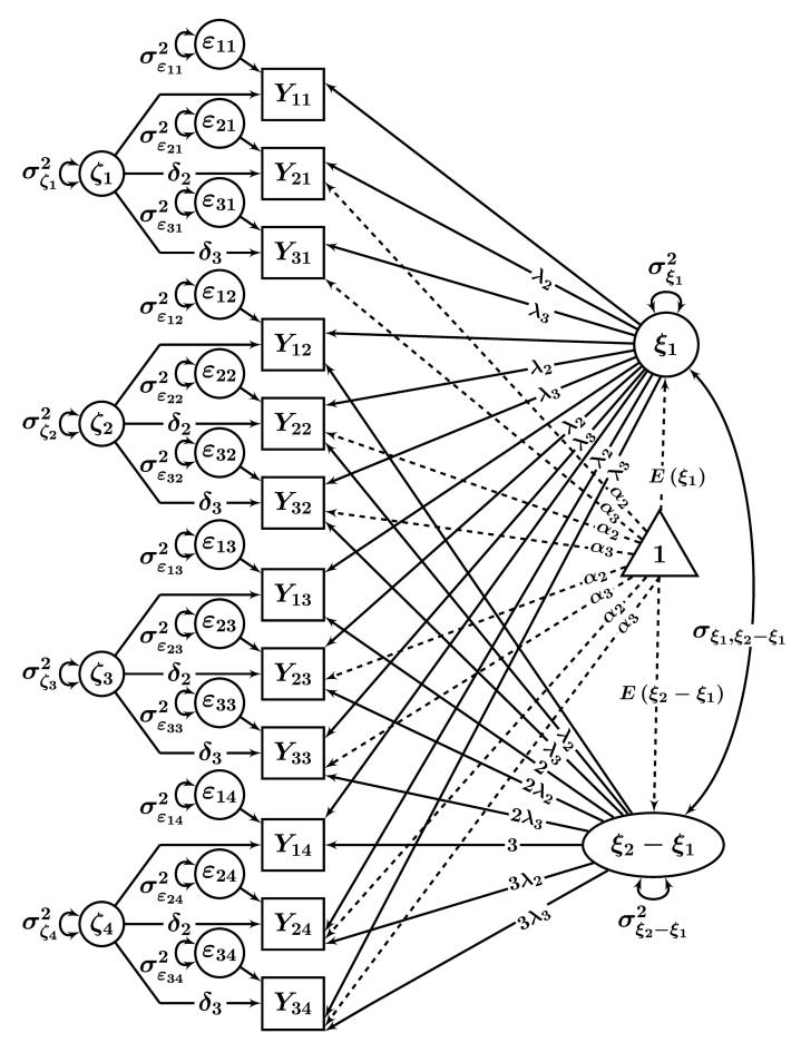
Figure 3 shows the multiple-indicator LGC model used here, assuming linear growth. (A formal derivation of this model based on concepts of LST theory is provided in Appendix A as well as in Bishop, Geiser, & Cole, 2013.) It can be seen that as in standard (single-indicator) linear LGC models, there is an intercept factor (ξ₁) that reflects individual differences in the initial (time 1) trait scores and a slope factor (ξ₂ − ξ₁) that reflects individual differences in linear trait change across time. Intercept and slope factor can be correlated.⁵

Figure 3.

Path diagram illustrating a multiple indicator linear LGC model for four time points with time-invariant parameters. The triangle represents a constant of 1 that symbolizes the mean structure in the model. The intercepts for the first indicator are set to zero (α₁ = 0) for identification and not explicitly shown in the figure. Loadings without a label are fixed to 1.

In contrast to single-indicator LGC models, the present model allows for multiple indicators at each time point. The indicators are allowed to have different intercepts and loadings within the same time point to account for potential differences in scaling. Using multiple indicators at each time point makes it possible to account for a state-variability process in this model in addition to the trait-change process that is reflected in the slope factor. The state-variability process is captured by the latent state residual factors ζ_it that have the same meaning as in the STMS model. With just a single indicator, the state variability process could not be separated from trait change and random measurement error (which represents a limitation of standard single-indicator LGC models).

The LGC model in Figure 3 can thus be seen as a hybrid model: It accounts for both a linear trait change process [reflected in the slope factor (ξ₂ − ξ₁)] and a state-variability process (reflected in the latent state residual factors ζ_t). The model in Figure 3 is more general than single-indicator LGC models, as it allows separating random measurement error from true state-variability processes. Furthermore, the STMS model can be viewed as a special case of this model. The LGC model in Figure 3 reduces to the STMS model if the latent trait-change component is zero, that is, if Var(ξ₂ − ξ₁) = (ξ₂ − ξ₁) = 0. In this case, all indicators measure a single time-invariant latent trait ξ₁ = ξ as in the STMS model, and there is no trait-change process.

Although not obvious at first sight, the model in Figure 3 is closely related to McArdle’s (1988) second-order or curve-of-factors LGC model for multiple indicators. The only difference between the model used here and the more commonly seen second-order LGC model is that the model in Figure 3 allows estimating the loadings on the latent state residual factors as independent model parameters (δ_it), whereas the same loadings are implicitly constrained to be equal to the trait loadings (λ_it) in McArdle’s model. We chose the more general model with independent state residual loadings here to make the relationship between the STMS model and multiple-indicator LGC models clearer. Nonetheless, the basic interpretation of this model is the same as in McArdle’s (1988) multiple-indicator LGC model.

In the linear LGC model, the means of the latent trait variables are given by:

$$\begin{array}{cc}\hfill E\left({\xi }_{it}\right)& =E\left({\alpha }_{it}\right)+E\left({\lambda }_{it}{\xi }_1\right)+E\left[{\lambda }_{it}\right(t-1\left)\right({\xi }_2-{\xi }_1\left)\right]\hfill \\ \hfill & ={\alpha }_{it}+{\lambda }_{it}E\left({\xi }_1\right)+{\lambda }_{it}(t-1)E({\xi }_2-{\xi }_1)\hfill \\ \hfill & ={\alpha }_{it}+{\lambda }_{it}E\left(intercept\right)+{\lambda }_{it}(t-1)E\left(Slope\right),\hfill \end{array}$$ (30)

for t = 1, …, n. Equation 30 shows us that, in contrast to the STMS model, in this linear LGC model, changes in the means of the latent trait variables over time can arise from three sources: (1) changes in the intercepts α_it, (2) changes in the trait loadings λ_it, and/or (3) true trait change as represented by the mean of the slope factor, E(ξ₂ − ξ₁). In other words, in this model, true changes in the means of the latent trait variables [as represented by E(ξ₂ − ξ₁)] can be separated from changes in the measurement parameters (α_it and λ_it). This is not possible in the STMS model, because this model assumes that there is no trait change.

A similar argument holds for changes in the variances of the latent trait variables, Var(ξ_it). In the linear LGC model, these variances can be expressed as:

$$\begin{array}{cc}\hfill Var\left({\xi }_{it}\right)& ={\lambda }_{it}^{2}Var\left({\xi }_1\right)+{\lambda }_{it}^2{(t-1)}^{2}Var({\xi }_2-{\xi }_1)+2{\lambda }_{it}^2(t-1)Cov[{\xi }_1,({\xi }_2-{\xi }_1\left)\right]\hfill \\ \hfill & ={\lambda }_{it}^{2}Var\left(Intercept\right)+{\lambda }_{it}^2{(t-1)}^{2}Var\left(Slope\right)+2{\lambda }_{it}^2(t-1)Cov(Intercept,Slope).\hfill \end{array}$$ (31)

As a consequence, changes in the latent trait variances can be due to (1) changes in the loadings λ_it, (2) true growth variance [as represented by Var(ξ₂ − ξ₁)], or (3) the growth factor covariance {as represented by Cov[ξ₁, (ξ₂ − ξ₁)]}.

In summary, even if α_it and λ_it are constrained to be time-invariant for all indicators in the LGC model (as would be recommended by most methodologists), mean and variance change over time is still allowed in the LCG model, because of the true trait-change component (ξ₂ − ξ₁). This feature distinguishes the LGC model from the STMS model, in which true trait change (if present) will be confounded with non-invariance of α_it, λ_it, or both. In other words, the LGC model clearly distinguishes true trait change from (usually undesirable) changes in the trait factor loadings and intercepts, whereas such a distinction cannot be made in the STMS model with non-invariant parameters.

In the hybrid model, the CO coefficient is defined as follows:

$$CO\left(Y_{it}\right)=\frac{{\lambda }_{it}^{2}Var\left(Intercept\right)+{\lambda }_{it}^2{(t-1)}^{2}Var\left(Slope\right)+2{\lambda }_{it}^2(t-1)Cov(Intercept,Slope).}{Var\left(Y_{it}\right)}.$$ (32)

As can be seen from Equation 32, both the intercept and slope contribute to the CO coefficient in the hybrid model, as both are related to the trait part of the model. The OS coefficient is defined in the same way as in the STMS model (see Equation 8) and Rel(Y_it) = OS(Y_it) + CO(Y_it).

Our description of the LGC model makes clear that if a true trait-change or a hybrid process generated the data (be it a linear or other growth process), it is preferable to analyze the data with an appropriate LGC or other kind of latent trait-change model rather than an LST model. The reason is that although an LST model with non-invariant parameters is able to capture trait change, it does so in a conceptually ambiguous way, that is, by allowing measurement-related parameters (α_it, λ_it) to be non-invariant. This is conceptually problematic because it confounds potential measurement non-invariance (i.e., measurement bias) with true change in the trait values. In contrast, the LGC model separates measurement (non)invariance issues from true trait change in the structural model. The LCG model is therefore preferred when the process under study involves trait change rather than or in addition to state-variability processes. The following simulation study demonstrates some consequences of fitting an LST model with non-invariant parameters to data generated by a trait-change process.

Simulation Study

Method

The purpose of this simulation was to (1) show that LST models with non-invariant parameters fit data generated by a trait-change process well across a wide range of conditions and (2) examine the problematic consequences of accepting LST models and interpreting the resulting parameter estimates for trait-change data. The purpose of the simulation is not to examine all possible constellations of non-invariance or trait change; rather, we use this simulation to illustrate the practical relevance of our analytical derivations through concrete examples. We defined several population models that not only included a state-variability process (in terms of a non-zero amount of occasion-specific variance), but also included (1) true changes in the latent trait means and (2) individual differences in trait change over time. The multiple-indicator LGC model introduced in the previous section (see Figure 3) served as the basis for generating the population data for three indicators (i = 3) measured on four measurement occasions (t = 4). As explained above, this model contains not only a true trait component (as represented by the latent intercept factor ξ₁) as in the STMS model, but also a true trait-change component [as represented by the linear slope factor (ξ₂ − ξ₁)]. In addition, latent state residual components (δ_itζ_t) at each time point reflect systematic state-variability in line with conventional LST models. In summary, this model can be seen as a hybrid, involving not only a state-variability process, but also (linear) changes in the trait scores over time.

In our simulation, we used nine different population models to show that the issues discussed in this paper hold across a range of conditions, including models with small and large amounts of trait change over time. The population models varied in terms of (1) the level of mean trait change over time as reflected in different latent slope factor means (we included three conditions of small, medium, and large mean differences according to Cohen’s [1988] conventions for effect sizes in terms of Cohen’s d) and (2) three levels of individual differences in trait change over time as reflected in different latent slope factor variances (we included conditions in which the latent slope factor variance was specified to be 1%, 5%, or 10% of the time 1 trait factor variance). State residual factor loadings in this model were specified as time-invariant (all loadings were fixed to 1). The exact population parameter specifications of the population LGC model are described in Appendix B.

Multivariate normal data were generated for each of the nine population models for four different sample size conditions (N = 250; N = 500; N = 1,000; and N = 5,000). We chose these sample sizes for the following reasons. First, we wanted to include a sample size that is found in typical LST applications. Geiser and Lockhart (2012) reviewed 57 LST applications and found a median sample size of N = 249 (68.4% of studies in their review used sample sizes ≤ 500). Second, we wanted to ensure that a seemingly good fit of an incorrectly specified model was not simply due to low statistical power, caused by small sample size. We therefore used three additional, larger sample size conditions (N = 500; N = 1,000; and N = 5,000) as well to demonstrate that even when power is very high, the chi-square test may not reliably identify an LST model with non-invariant parameters as incorrect for data derived from a true population model of change.

We generated 1,000 replications for each cell of the design using Mplus 6 (Muthén & Muthén, 1998-2012). We then analyzed the data in Mplus with (1) the correctly specified multiple-indicator linear LGC model that generated the data (i.e., the true population model shown in Figure 3), (2) the STMS model with non-invariant parameters, (3) the STMS model with weak factorial invariance (i.e., time-invariant trait and state residual factor loadings, but non-invariant intercepts, and (4) the STMS model with strong factorial invariance (i.e., time-invariant trait and state-residual factor loadings and invariant intercepts). In total, we conducted 3 (slope factor mean) × 3 (slope factor variance) × 4 (sample size) × 4 (model type) × 1,000 (replications) = 144,000 analyses.

We hypothesized that the data-generating LGC model would fit the data well and produce unbiased parameter estimates under all conditions, given that (1) it was the true model and (2) even the lowest sample size condition (N = 250) appeared large enough to produce dependable parameter estimates. We further hypothesized that the STMS model with non-invariant parameters would fit the data reasonably well in terms of the chi-square test or at least in terms of criteria for approximate model fit that are commonly used in practice (Hu & Bentler, 1999; Schermelleh-Engel, Moosbrugger, & Müller, 2003). Even though the STMS model with non-invariant parameters was clearly different from the data-generating trait-change model, we expected it to fit the data adequately, given that it allowed all factor loadings and intercepts to vary freely across time. As we showed in the analytic section, these parameters can capture not only mean changes but (to some extent) changes in the variances of the latent trait variables across time. In fact, leaving the intercepts free for all indicators implies a saturated mean structure.

For the STMS weak factorial invariance specification, we expected that this model would lead to more correct rejections (misfit), albeit not as many as a strong factorial invariance model. Finally, we hypothesized that the STMS model with strong factorial invariance would not fit the data well under any condition, given that it involves time-invariant factor loadings and intercepts and thus does not account for trait changes over time. Hence, the STMS model with invariant parameters (but not the STMS model with non-invariant parameters) was expected to clearly reveal the misspecification that arises from fitting a pure state-variability model to a trait-change process.

In each condition, we also examined parameter bias in the coefficients that are typically of interest in an LST analysis, namely the CO, OS, and Rel coefficients for all models relative to the true population models. This step should reveal the potentially dangerous consequences of accepting a pure state-variability model for data that were actually generated by a trait-change process. We expected the coefficients of consistency and occasion-specificity to be biased in the STMS models with either invariant and non-invariant parameters, as both models are misspecified relative to the population model. Specifically, we hypothesized that STMS models with non-invariant or only weakly invariant parameters would erroneously attribute trait-change variance to occasion-specific variability and thus lead to a systematic underestimation of consistency and an overestimation of occasion-specificity.

Results

Model convergence and improper solutions

All models converged under all conditions. In terms of improper solutions (“Heywood cases”), not a single replication resulted in an improper residual covariance matrix (negative indicator residual variances). However, 1,575 analyses (1.1% of all analyses) yielded non-positive definite latent variable covariance matrices. All of these cases occurred in analyses of the true population model (i.e., the correctly specified case), implying that 4.4% of analyses for this model were improper. The vast majority (1,560 = 99%) of these cases were in the small slope factor variance condition, whereas the remaining 15 (1%) were in the medium slope factor variance condition. In addition, the frequency of non-positive definite latent variable covariance matrices was negatively correlated with sample size (786 cases [49.9%] in the N = 250 condition; 510 [32.4%] in the N = 500 condition; 279 [17.7%] in the N = 1,000 condition, and zero in the N = 5,000 condition).

Given that the true population value of the slope factor variance was close to zero in this condition, the straightforward explanation is that sampling error was more likely to yield slope factor variance estimates of zero (or even slightly below zero), compared to the other conditions, in which the population slope factor variance was farther away from zero. In the larger sample size conditions, the problem was less severe, because sampling error was reduced.

Model fit

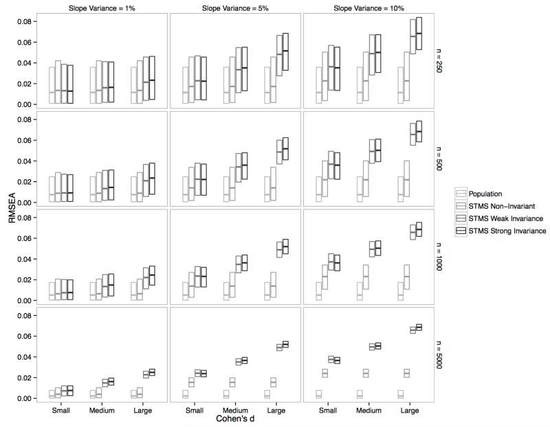
We analyzed the absolute fit of all models in terms of (1) exact model fit and (2) approximate model fit as is commonly done in the literature (e.g., Hu & Bentler, 1999; Schermelleh-Engel et al., 2003). We categorized a model as not being rejected according to a test of exact model fit when the chi-square test was non-significant (p > .05) for the model. In terms of approximate fit, we examined the Root Mean Square Error of Approximation (RMSEA; Steiger, 1990), Comparative Fit Index (CFI; Bentler, 1990), and Standardized Root Mean Square Residual (SRMR; Schermelleh-Engel et al., 2003). To simplify the presentation, we defined a summary fit criterion according to which a model was seen as acceptable if jointly RMSEA ≤ .05, CFI ≥ .95, and SRMR ≤ .05. (Note that we still present the results for each individual fit index in Appendix D.) ⁶

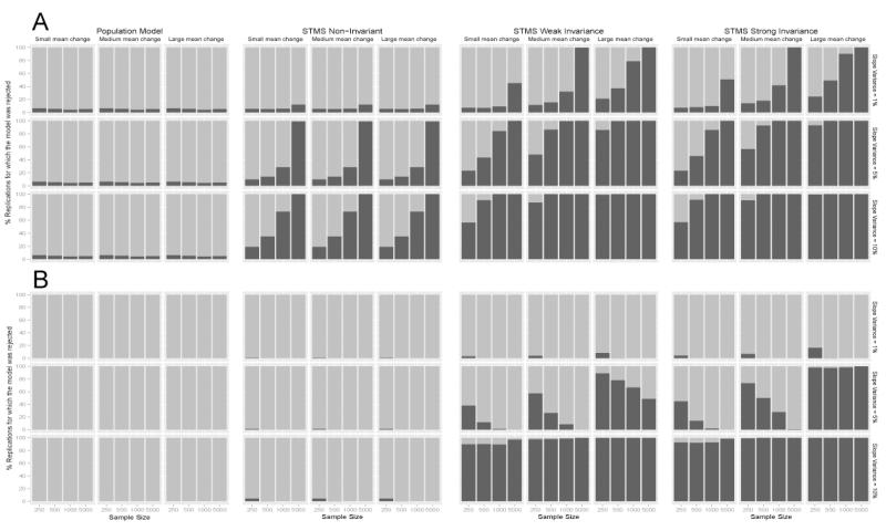
The black bars in Figure 4A show the percentage of replications in each condition that had a non-significant chi-square test of model fit (p > .05) and thus would be seen as satisfying the criterion of exact model fit. The black bars in Figure 4B show the percentage of replications meeting the criterion for approximate fit. The true population model was consistently rejected only in about 5% of cases according to the chi-square test of model fit. This rejection rate is commensurate with an alpha error rate of 5%. Moreover, the population model met the approximate fit criteria in 100% of cases.

Figure 4.

Proportion of replications meeting goodness-of-fit criteria for each of the 4 (analysis models) × 36 (simulation conditions) = 144 cells of the simulation study. A: Exact fit. B: Approximate fit.

More interestingly, and as expected, the STMS model with non-invariant parameters also showed a good fit under a wide range of conditions. According to the chi-square test, the rejection rate for this model was only about 5% in the small slope-factor variance conditions when the sample size was N = 1,000 or below, and only about 10% in the N = 5,000 condition. In the medium slope-factor variance condition, the rejection rate was still relatively low for the three smaller sample size conditions, but was 100% in the N = 5,000 condition. In the largest slope-factor variance condition, the rejection rate was still below 20% in the N = 250 condition and below 40% in the N = 500 condition. Importantly, the misspecified STMS model with non-invariant parameters met the criteria for acceptable approximate fit in almost 100% of cases across all conditions. In summary, researchers using exact fit statistics may retain this model in many instances, and researchers relying exclusively on approximate fit indices would have retained this model under virtually all conditions studied in this simulation.

Figure 4 also illustrates that the rejection rate for this model did not vary across different levels of mean change. This is expected, given that the STMS model with non-invariant parameters does not place restrictions on the observed mean structure. Therefore, regardless of whether mean changes over time are small or large, the model can fit these changes by varying intercept parameters across time.

The STMS model with weak invariance showed an overall higher rejection rate compared to the non-invariant model. Especially with large samples and medium to high slope variance, the model was consistently rejected according to the chi-square test of exact fit. On the other hand, this model yielded a relatively high rate of acceptable chi-square p-values in the smaller sample size conditions (250 and 500) for small to medium slope mean and variance. Approximate fit criteria were almost completely insensitive to the misspecification in the smallest slope variance conditions and would have let to a high rate of incorrect model acceptance also in the medium slope variance condition. Only in the large slope variance conditions did approximate fit indices consistently reject the weak invariance model.

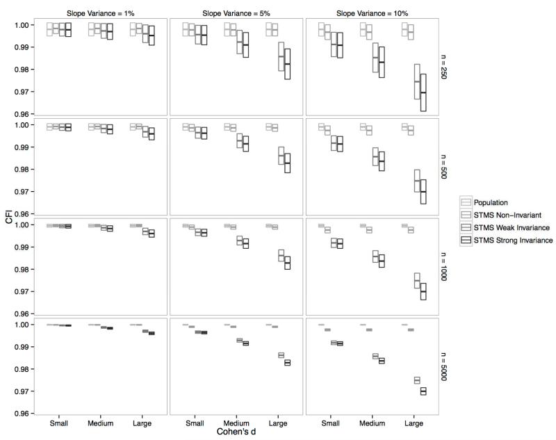
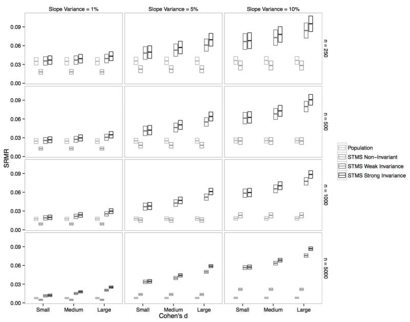
As expected, the STMS model with strong invariance (time-invariant loadings and intercepts) showed higher rejection rates than the weak and non-invariance models. The strong invariance model was consistently rejected by the χ² test when slope-factor variance and mean were at least of moderate size. However, even the time-invariant model had χ² rejection rates below 20% in the small slope-factor variance condition when mean change was of small or medium size and the sample size was 500 or lower. Sample sizes ≥ 500 were needed to achieve a rejection rate > 50% in the moderate slope-factor variance/small mean change condition. Approximate fit was acceptable in many cases for small and moderate slope-factor variance, whereas for the large slope-factor variance conditions, and the medium slope variance conditions with large mean change, approximate fit criteria led to model rejection in most cases. Analyses of individual fit statistics (see Appendix D) revealed that this rejection was entirely driven by RMSEA and SRMR, whereas CFI was completely > 0.97 and thus showed no sensitivity to the misspecification. In line with Marsh, Hau, and Wen (2004), we found that the probability of correctly rejecting a misspecified model based on approximate fit indices decreased with increasing sample size. This relation was particularly obvious for the STMS models with weak and strong invariance.

Parameter bias

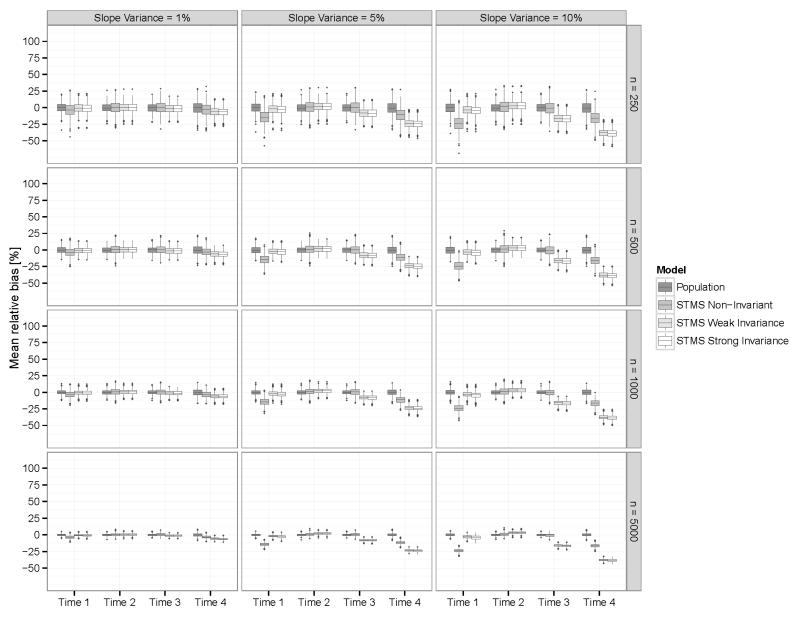
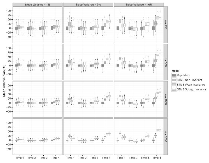
Figures 5 and 6 show the percent average parameter bias in the estimation of the consistency and occasion-specificity coefficients relative to the true population values, respectively. Note that the values represent aggregates across the three indicators within each occasion. Further note that in the population growth model, consistency is defined as the proportion of variance in the observed indicators that is accounted for by trait and trait change (Eid et al., 2012). The population model accurately reproduced both types of coefficients on average (i.e., average bias differed only marginally from zero in all conditions for the data-generating model). In contrast, both the STMS model with non-invariant parameters and the STMS model with invariant parameters showed bias in the estimation of the consistency and occasion-specificity coefficients in the medium and large slope factor variance conditions. Contrary to our expectations, the bias in occasion-specificity in the LST model with non-invariant parameters was highest for the first and the last time point. For both of these time points, occasion-specificity tended to be overestimated. Bias in occasion-specificity for the model was substantial and ranged from roughly 25% in the medium slope-factor variance condition to up to approximately 37% in the large slope-factor variance condition. As one would expect, biased estimates also occurred in the LST model with time-invariant parameters (because this model was clearly misspecified for the population data). Reliability estimates were largely unbiased for all three models under all conditions, so that we did not include a separate graph for reliability bias.

Figure 5.

Average bias in the coefficients of consistency for the three four used in the simulation study.

Figure 6.

Average bias in the coefficients of occasion-specificity for the four models used in the simulation study.

Discussion of Simulation Results

The purpose of the simulation study was to illustrate that, under a variety of conditions, an LST model with non-invariant parameters can provide a disturbingly good fit to data that actually involve a trait-change process (and not just state variability). A lack of statistical power can be excluded as an explanation for the remarkably good chi-square values for the LST model with non-invariant parameters, given that we included large sample sizes of N ≥ 500. In practice, LST applications often involve sample sizes well below N = 500 or even N = 250 (Geiser & Lockhart, 2012). Hence, we may assume that the issues demonstrated here are even more problematic in many applied LST studies. Investigators using LST models with non-invariant parameters may not notice that there is actually a trait-change process in their data even when this effect is strong—as demonstrated by the remarkably good fit even in conditions that involved strong trait changes over time. This problem will be exacerbated to the extent that researchers ignore the mean structure in LST analyses. In these cases, even when factor loadings are specified as time-invariant, mean changes across time could still occur and would not result in a bad fit, given that an LST model with non-invariant intercepts has a saturated mean structure. As a consequence, investigators may not notice such changes based on model fit criteria.

Of note, even though LST models with time-invariant loadings and/or intercepts showed much higher rates of correct rejections than the LST model with non-invariant parameters, these models were not consistently rejected by approximate fit statistics unless individual differences in trait change over time were at least 5% of the initial trait factor variance and mean change was large. This demonstrates once again that researchers need to be cautious in accepting pure state-variability models when there may be actual trait changes. Particular problems may arise in this context from the use of approximate fit criteria in large samples, because of the negative relation between correct model rejection and sample size found for approximate fit indices. This counter-intuitive relation was discussed by Marsh et al. (2004) for SEMs in general and replicated for LST models in the present study. We also showed that the incorrect acceptance of a state-variability model for data actually generated by a trait-change process can result in biased coefficients of consistency and occasion-specificity, which are typically the main focus of applied LST studies.

General Discussion

Researchers in psychology and other social sciences frequently ask the question of whether the longitudinal course of a construct is most appropriately described as state variability (i.e., short-term and typically reversible changes in individual’s true state scores that fluctuate around an invariant trait level) or trait change (i.e., long-term and typically irreversible modifications to individual’s trait scores). Whereas LST models are designed to model state-variability processes around an invariant trait LGC models are designed to model trait-change processes. In addition, in this manuscript we highlighted the value of hybrid models, which combine features of both, LST and LGC models (Tisak & Tisak, 2000). In our discussion, we first summarize the key findings of this paper. Subsequently, we provide detailed procedural advice for researchers studying variability and change in longitudinal data.

Summary of Findings

Traditionally, methodologists and applied longitudinal researchers have regarded the MI issue as mainly a problem of avoiding “measurement bias”. In other words, researchers’ main focus in testing for MI in longitudinal data has usually been on whether the psychometric properties of measured variables and/or their meaning have changed over time. In this article, we demonstrated that testing MI is not only a question of measurement bias, but that it is also relevant for distinguishing state variability from trait change processes in longitudinal data. Specifically, we showed that LST models, which are designed to measure state-variability processes, can capture various forms of trait change if these models are specified with non-invariant measurement intercept and/or loading parameters. This is true even if no measurement bias is present.

Hence, not testing for MI in LST analyses can not only mask a potential measurement problem, but can also lead to difficulties in empirically distinguishing a state-variability from a trait-change process. Our simulation study illustrated this problem, showing that researchers fitting LST models with non-invariant parameters to data generated by a latent trait-change process may obtain a well-fitting solution and erroneously conclude that the process is best described as a pure state-variability process. In other words, by fitting an LST model with non-invariant parameters, a researcher may miss the fact that the longitudinal course of the construct under study actually involves trait changes instead of, or in addition to, state variability. In summary, measurement non-invariance poses problems in LST analyses whenever a key question is whether the longitudinal dynamics of a construct are best described by a state-variability (i.e., state-trait) process, a trait change process, or both.

Our paper should not be read as suggesting that LST models are problematic in general or that these models should not be used. On the contrary, we think that LST models are extremely valuable models for analyzing state-variability processes in psychological attributes and that longitudinal researchers should have these models in their tool boxes. Our concern here is that many applications of LST models to date have not considered issues of MI in the analysis of these models, probably because the meaning and consequences of non-invariant measurement parameters in LST models were not clear to most researchers. As a consequence, many studies may have erroneously concluded that the process that they study is a pure state-variability process. Hence, the issue is not that LST models are not useful; rather, the issue is that they should be properly applied. Below we provide four tips for the proper use of LST models.

Tip #1: Carefully Test for MI in LST Analyses

We recommend that researchers using LST models should establish at least strong factorial invariance in their LST models. For this purpose, the global model fit in terms of the chi-square fit test of constrained models with equal intercepts (α) and equal loadings (λ) on the trait factor(s) should be examined. In addition, we recommend that researchers test constrained models against less constrained models that allow for time-varying intercepts or trait loadings. Given that such models are nested, they can be tested against each other directly using chi-square difference tests, provided the less restrictive model with non-invariant parameters fits the data. If MI models do not fit the data well and/or if they fit the data worse than non-MI models, researchers should carefully consider the possibility that the process under investigation may be better described by a trait-change model (see “Tip 4” below). Another potential explanation for measurement non-invariance can be the so-called Socratic effect (e.g., Jagodzinski, Kühnel, & Schmidt, 1987), according to which individuals oftentimes need to get used to the measurement instrument. This effect may cause the measurement model to be different at Time 1 compared to the remaining time points, without trait change being present. Running analyses with and without the Time 1 data can help examining this possibility.

In addition, even when full MI does not hold, the assumption of partial MI may be tenable (e.g., Cheung & Rensvold, 1999). Partial MI means that the measurement parameters (e.g., factor loadings or intercepts) are time-invariant for some but not all observed variables. Strategies for testing partial MI statistically have been described in Byrne, Shavelson, and Muthen (1989) as well as Cheung and Rensvold (1999). In the context of LST models, partial MI could imply that some indicators measure a stable trait, whereas others measure a slightly different trait that changes across time. Under “Tip #4” we describe alternative models that may be considered in cases of partial or full measurement non-invariance.

Researchers may wonder whether loading invariance is equally important on the side of the latent state residual factors. Even though invariance of the state residual factor loadings (δ) is not critical for the proper interpretation of trait changes, such non-invariance may indicate a violation of a fundamental assumption made in LST theory (Steyer et al., 1992). LST theory assumes that the situations are drawn at random from a set of exchangeable situations at each time point. Changes in the latent state residual factor loadings may thus indicate that the situations were not exchangeable and that a standard LST model may not be the best model to use. Instead, a model that uses one situation as reference and contrasts the remaining situations against this reference may be more appropriate in these cases. Such a model was discussed by Schermelleh-Engel, Keith, Moosbrugger, and Hodapp (2004).

Tip #2: Include and Analyze the Mean Structure in LST Analyses

In line with the previous recommendations about testing loadings and intercepts for MI, researchers should routinely include the mean structure in their LST analyses, even when the mean structure does not appear to be of substantive interest. Including the mean structure in an LST analysis allows researchers to test the assumption of strong MI. If the intercepts are not time-invariant, this may be a sign that mean changes have taken place over time, again providing evidence against a pure state-variability process.

The relevance of testing mean structures in LST models may be surprising to many researchers, given that LST models have often been presented and interpreted as pure covariance structure models, focusing on variance components and the estimation of consistency, occasion-specificity, and reliability coefficients. We may speculate that mean structures were deemed irrelevant to LST analyses by many researchers, as means are not needed for the computation of the above coefficients. Consequently, the time-invariance of intercepts has rarely been explicitly tested in LST applications. ⁷

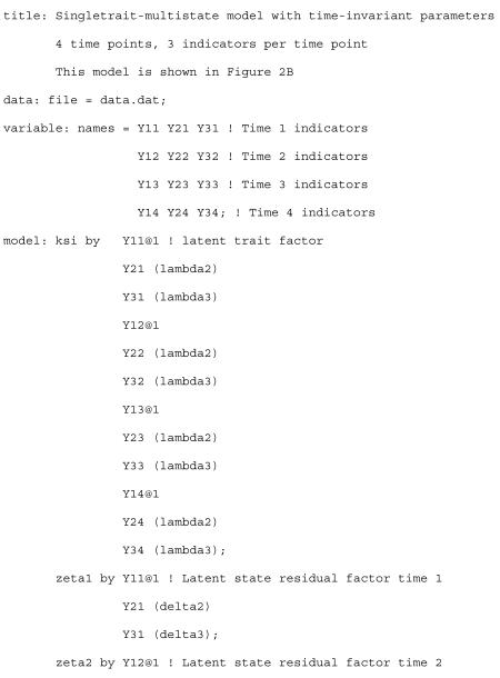
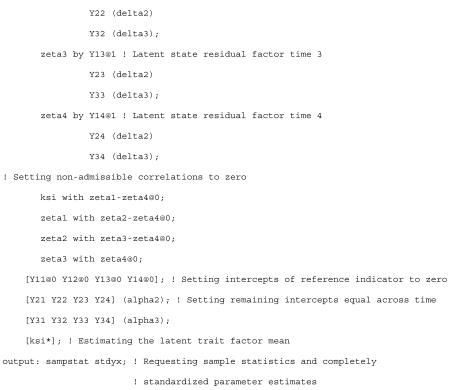
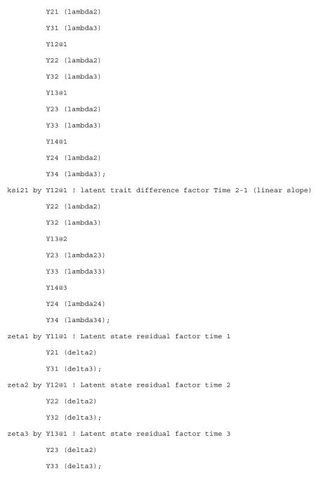
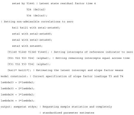
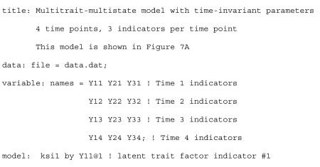
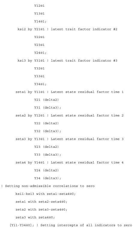
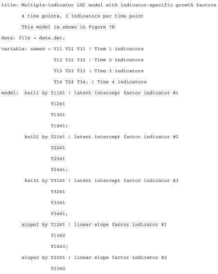
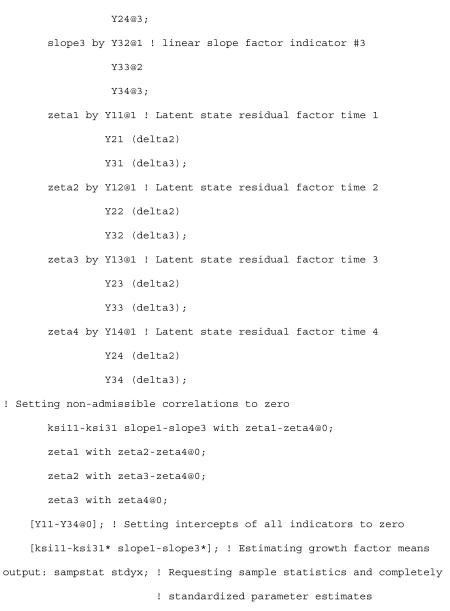
Even though mean structures may not be of direct substantive interest in LST studies, including them into the analysis is critical. Without a mean structure, MI cannot be fully tested. If the mean structure is not included in the model, potential trait changes may be overlooked, because a model with free intercepts implies a saturated mean structure that cannot cause misfit in the model. We reiterate here that SEM computer programs may include (non-invariant) intercepts into the model by default. Researchers should be aware of the fact that this default specification can mask trait changes in an LST model. In Appendix C, we provide a sample Mplus script showing the correct mean structure specification in the STMS model.

Tip #3: Avoid Small Designs

Many previous applications of LST models used only two indicators (“test halves” or item parcels) measured on just two measurement occasions (we refer to such designs as 2 × 2 designs). In many of these applications, item parcels were specifically created to be homogenous (i.e., tau-equivalent in the sense of CTT), and hence all factor loadings were fixed (typically to 1) at all time points. A model of tau-equivalence (or essential tau-equivalence) implies time-invariant loadings (because all loadings are 1 at each time point), such that the issue of loading invariance does not require specific attention in these cases.

Although small designs are useful to demonstrate the minimal conditions under which LST models can be applied, these designs make it harder to test certain invariance assumptions and to detect trait changes over time. For example, in a 2 × 2 design, the constraint of equal state residual factor loadings at each time point is required for model identification and thus does not represent a testable constraint (unless the latent state residual factors are correlated with external variables). Furthermore, at least one trait factor loading must be set equal across time for identification reasons. Hence, 2 × 2 designs are particularly problematic because they make it more difficult for researchers to detect potential violations of MI. Such small designs also make it difficult to distinguish short-term fluctuations from actual trait changes, especially when the spacing of measurement occasions is closely adjacent in time. Moreover, the use of a small number of indicators (i.e., nearly underidentified models) in conjunction with small samples may result in low statistical power to detect violations of invariance assumptions and detect individual differences in trait changes (e.g., von Oerzen et al., 2008).

In summary, even though small designs are sufficient to estimate the CO, OS, and Rel coefficients and may be useful, researchers should generally avoid these kinds of designs if possible. We recommend that researchers include at least three indicators in their analyses and collect data for the same indicators on four or more time points (Ciesla et al., 2007). Such larger designs allow for more powerful tests of the assumption that the process under investigation is a pure state-variability (state-trait) process.

Tip #4: Consider and Test Alternative Models

Although LST models are useful for modeling the longitudinal course of a range of psychological constructs, researchers should always consider alternative models as well. In particular, we recommend that researchers compare the fit of LST models to the fit of hybrid models that allow for trait change in addition to state variability. Eid and Hoffman (1998), Eid et al. (2012), as well as Tisak and Tisak (2000) provided modeling frameworks for such hybrid cases. In Appendix C, we included a sample Mplus script showing the proper specification of the hybrid linear growth model presented in this paper. Different hybrid models were also discussed in detail by Bishop et al. (2013).

Testing alternative models that allow for a trait-change component is especially important when a researcher has found an LST model with strong factorial invariance to not fit well. In these cases, the researcher can first try to fit an alternative invariant LST model, in which some of the restrictive assumptions of the STMS model are relaxed to examine whether the lack of fit is related to method effects (indicators showing correlated residuals across time) rather than the presence of trait changes. For this purpose, we recommend that researchers fit an LST model with indicator-specific traits (see Figure 7A) if the STMS model is rejected by fit statistics. This model is also known as multitrait-multistate (MTMS) model, as it allows each indicator to have its own trait factor. The MTMS model relaxes the assumption of perfectly correlated trait variables ξ_it made in the STMS model, thus allowing for method effects (indicator-specificity) across time (an Mplus script for the proper specification of the MTMS model can be found in Appendix C; for a more detailed description of the model, see Geiser & Lockhart, 2012).

Figure 7.

Models with indicator-specific trait and trait change factors to account for method effects. A: Multitrait-multistate (MTMS) model. B: Multiple-indicator linear LGC model with indicator-specific intercept and slope factors. All intercepts are fixed to zero and not explicitly shown in the figure. Loadings without a label are fixed to 1.

If also the MTMS model does not provide a reasonable fit to the data, it is likely that indicator-heterogeneity alone cannot explain the misfit of LST models to the data. Instead, trait-change may be present in addition to a state-variability process. In this case, the researcher should first assess whether some or all indicators show non-invariant parameters across time. The MTMS model can be extended to include growth factors for some or all indicators, depending on whether non-invariance is partial or concerns all indicators (see Figure 7B for a linear growth model with indicator-specific growth factors for all indicators; a sample Mplus script is available from Appendix C; for a more detailed description of indicator-specific LGC models, see Bishop et al., 2013). In addition to linear growth, researchers may try more complex growth or hybrid models that either specify more complex forms of growth (e.g., quadratic) or estimate the form of growth freely from the data (e.g., Tisak & Tisak, 2000).

Conclusion

The previous literature in the field of LST modeling has not sufficiently emphasized the fact that testing MI is an important step in distinguishing state-variability from trait-change processes in longitudinal data. We urge researchers applying LST models to (1) include a mean structure in the analysis and (2) conduct and report explicit tests of MI for both the factor loadings and intercepts. Even when an LST model with time-invariant parameters fits our data, we cannot be absolutely certain that the process is best described as a pure state-variability process in general. Too few indicators, time points, or participants may diminish power to detect misspecifications of such a model. Furthermore, a psychological process may be adequately described as a pure state-variability process across a certain period of the life span, but may be subject to actual trait changes during other periods of life. We hope that our guidelines will help improve longitudinal research by sharpening the conceptual and empirical distinction between state-variability and trait-change processes and by helping researchers to apply LST models appropriately.

Figure D1.

Mean RMSEA (middle of the box) and 90% confidence limits (upper and lower limits of the box) across the simulation conditions.

Figure D2.

Mean CFI (middle of the box) and SD (upper and lower limits of the box) across the simulation conditions.

Figure D3.

Mean SRMR (middle of the box) and SD (upper and lower limits of the box) across the simulation conditions.

Appendix A

Formal Definition of the Multiple-Indicator LGC Model Used in the Simulation Study

The multiple-indicator linear LGC model used in the simulation study (see Figure 3) was first presented by Eid, Courvoisier, and Lischetzke (2012). Here, we show how this model can be formally defined based on concepts of LST theory to illustrate its mathematical relationship to the STMS model. For more details, see Bishop, Geiser, and Cole (2013). In the first step, we assume that all latent trait variables measured at the same time point t are congeneric:

$${\xi }_{it}={\alpha }_{it}+{\lambda }_{it}{\xi }_t.$$ (A1)

This is different from the assumption stated in Equation 3 for the STMS model in that we no longer postulate homogeneity of all latent trait variables ξ_it but only of those that are measured on the same time point t. In the second step, we define an intercept factor to be equal to the common latent trait factor measured at Time 1 (ξ₁) and a slope factor to be equal to the latent difference variable (ξ₂ − ξ₁):

$$Intercept\equiv {\xi }_1$$ (A2)

$$Slope\equiv ({\xi }_2-{\xi }_1).$$ (A3)

In the third step, we make the assumption that change over time is linear by postulating the following relation:

$$\begin{array}{cc}\hfill {\xi }_t& ={\xi }_1+(t-1)({\xi }_2-{\xi }_1)\hfill \\ \hfill & =Intercept+(t-1)Slope.\hfill \end{array}$$ (A4)

In the fourth step, we assume as in the STMS model that occasion-specific effects are homogeneous for all indicators measured at the same time point, so that they can be represented by common state residual factors (compare Equation 4):

$${\zeta }_{it}={\delta }_{it}{\zeta }_t.$$ (A5)

Inserting Equation A4 into Equation A1, we obtain

$$\begin{array}{cc}\hfill {\xi }_{it}& ={\alpha }_{it}+{\lambda }_{it}{\xi }_t\hfill \\ \hfill & ={\alpha }_{it}+{\lambda }_{it}[{\xi }_1+(t-1\left)\right({\xi }_2-{\xi }_1\left)\right]\hfill \\ \hfill & ={\alpha }_{it}+{\lambda }_{it}{\xi }_1+{\lambda }_{it}(t-1)({\xi }_2-{\xi }_1)\hfill \\ \hfill & ={\alpha }_{it}+{\lambda }_{it}Intercept+{\lambda }_{it}(t-1)Slope.\hfill \end{array}$$ (A6)

Inserting Equations A5 and A6 into the basic LST measurement equation (Equation 5) yields

$$\begin{array}{cc}\hfill Y_{it}& ={\xi }_{it}+{\zeta }_{it}+{\epsilon }_{it}\hfill \\ \hfill & ={\alpha }_{it}+{\lambda }_{it}{\xi }_1+{\lambda }_{it}(t-1)({\xi }_2-{\xi }_1)+{\delta }_{it}{\zeta }_t+{\epsilon }_{it}\hfill \\ \hfill & ={\alpha }_{it}+{\lambda }_{it}Intercept+{\lambda }_{it}(t-1)Slope+{\delta }_{it}{\zeta }_t+{\epsilon }_{it}.\hfill \end{array}$$ (29)

The STMS model is a special case of the model in Equation 29 that results if Var(ξ₂ − ξ₁) = E(ξ₂ − ξ₁) = 0.

Appendix B

Parameter Specification in the Simulation Study

In this appendix, we describe the parameter specification of the population model used in the simulation study.

Parameter	Value
Indicator intercepts, αit	Fixed to 0 for all indicators
Loadings on the latent intercept factor, λξ1	Fixed to 1 for all indicators
Loadings on the linear slope factor, λ(ξ2−ξ1)	Fixed to 0 (time 1), 1 (time 2), 2 (time 3), 3 (time 4)
Loadings on the latent state residual factors, δit	Fixed to 1 for all indicators
Indicator residual variances, Var(εit)	Varied depending on the slope factor variance so that reliability would equal .8 for all indicators at all time points in all conditions
Variance of the intercept factor, Var(ξ1)	0.5
Mean of the intercept factor, E(ξ1)	0
Variance of the linear slope factor, Var (ξ2−ξ1)	Three conditions: 0.005 (1% of the intercept factor variance), 0.025 (5% of the intercept factor variance), and 0.05 (10% of the intercept factor variance)
Mean of the linear slope factor, E(ξ2−ξ1)	Varied depending on the slope factor variance condition to obtain small (0.2), medium (0.5), and large (0.8) mean differences in terms of Cohen’s d measure, respectively; Cohen’s d was defined as E(ξ2−ξ1)/[Var(ξ2−ξ1)0.5]
Covariance between intercept and linear slope factor, Cov[ξ1, (ξ2−ξ1)]	Fixed to 0
Latent state residual factor variances, Var(ζt)	Always 0.3 at time 1. Remaining values were varied depending on the slope factor variance condition, so that occasion-specificity would equal .3 for all indicators at all time points in all conditions
Covariances among latent state residual factors and between latent state residual factors and all other factors	Fixed to 0

Appendix C

Mplus Scripts for the Proper Specification of the STMS and Linear Growth Models With Time-Invariant Factor Loadings and Intercepts

STMS Model With Time-Invariant Parameters

Linear LGC Model With Time-Invariant Parameters

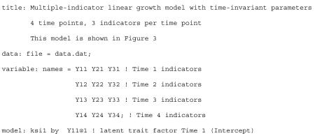
MTMS Model With Time-Invariant Parameters

Multiple-Indicator Linear LGC Model With Indicator-Specific Intercept and Slope Factors

Appendix D

Simulation Results for Individual Fit Statistics

Table D1. Mean χ² and SD for Each Cell of the Simulation Design.

Slope variance	Cohen’s d	Sample size	Model	df	χ2 mean	χ2 SD
1%	Small	250	Population	70	71.31	11.85
1%	Small	250	STMS Non-Invariant	42	43.22	9.16
1%	Small	250	STMS Weak Invariance	60	62.21	11.23
1%	Small	250	STMS Strong Invariance	66	68.37	11.66
1%	Small	500	Population	70	70.55	11.85
1%	Small	500	STMS Non-Invariant	42	42.60	9.20
1%	Small	500	STMS Weak Invariance	60	62.10	11.25
1%	Small	500	STMS Strong Invariance	66	68.60	11.85
1%	Small	1000	Population	70	70.30	11.37
1%	Small	1000	STMS Non-Invariant	42	42.91	9.16
1%	Small	1000	STMS Weak Invariance	60	63.77	11.12
1%	Small	1000	STMS Strong Invariance	66	70.48	11.86
1%	Small	5000	Population	70	69.85	11.67
1%	Small	5000	STMS Non-Invariant	42	45.79	10.14
1%	Small	5000	STMS Weak Invariance	60	78.42	13.96
1%	Small	5000	STMS Strong Invariance	66	87.56	14.77
1%	Medium	250	Population	70	71.31	11.85
1%	Medium	250	STMS Non-Invariant	42	43.22	9.16
1%	Medium	250	STMS Weak Invariance	60	64.59	11.76
1%	Medium	250	STMS Strong Invariance	66	71.59	12.20
1%	Medium	500	Population	70	70.55	11.85
1%	Medium	500	STMS Non-Invariant	42	42.60	9.20
1%	Medium	500	STMS Weak Invariance	60	66.98	12.15
1%	Medium	500	STMS Strong Invariance	66	75.11	12.98
1%	Medium	1000	Population	70	70.30	11.37
1%	Medium	1000	STMS Non-Invariant	42	42.91	9.16
1%	Medium	1000	STMS Weak Invariance	60	73.60	12.89
1%	Medium	1000	STMS Strong Invariance	66	83.63	14.02
1%	Medium	5000	Population	70	69.85	11.67
1%	Medium	5000	STMS Non-Invariant	42	45.79	10.14
1%	Medium	5000	STMS Weak Invariance	60	127.21	20.08
1%	Medium	5000	STMS Strong Invariance	66	153.33	22.24
1%	Large	250	Population	70	71.31	11.85
1%	Large	250	STMS Non-Invariant	42	43.22	9.16
1%	Large	250	STMS Weak Invariance	60	69.03	12.60
1%	Large	250	STMS Strong Invariance	66	77.55	13.13
1%	Large	500	Population	70	70.55	11.85
1%	Large	500	STMS Non-Invariant	42	42.60	9.20
1%	Large	500	STMS Weak Invariance	60	75.97	13.61
1%	Large	500	STMS Strong Invariance	66	87.13	14.75
1%	Large	1000	Population	70	70.30	11.37
1%	Large	1000	STMS Non-Invariant	42	42.91	9.16
1%	Large	1000	STMS Weak Invariance	60	91.66	15.56
1%	Large	1000	STMS Strong Invariance	66	107.78	17.18
1%	Large	5000	Population	70	69.85	11.67
1%	Large	5000	STMS Non-Invariant	42	45.79	10.14
1%	Large	5000	STMS Weak Invariance	60	217.20	27.91
1%	Large	5000	STMS Strong Invariance	66	274.15	31.43
5%	Small	250	Population	70	71.29	11.82
5%	Small	250	STMS Non-Invariant	42	45.62	9.62
5%	Small	250	STMS Weak Invariance	60	70.23	12.77
5%	Small	250	STMS Strong Invariance	66	76.82	13.18
5%	Small	500	Population	70	70.54	11.85
5%	Small	500	STMS Non-Invariant	42	47.38	10.21
5%	Small	500	STMS Weak Invariance	60	77.99	13.81
5%	Small	500	STMS Strong Invariance	66	85.30	14.41
5%	Small	1000	Population	70	70.29	11.35
5%	Small	1000	STMS Non-Invariant	42	52.37	11.10
5%	Small	1000	STMS Weak Invariance	60	95.31	15.87
5%	Small	1000	STMS Strong Invariance	66	103.70	16.58
5%	Small	5000	Population	70	69.84	11.67
5%	Small	5000	STMS Non-Invariant	42	93.41	17.20
5%	Small	5000	STMS Weak Invariance	60	237.01	29.55
5%	Small	5000	STMS Strong Invariance	66	254.69	30.64
5%	Medium	250	Population	70	71.29	11.82
5%	Medium	250	STMS Non-Invariant	42	45.62	9.62
5%	Medium	250	STMS Weak Invariance	60	79.79	14.49
5%	Medium	250	STMS Strong Invariance	66	89.35	15.12
5%	Medium	500	Population	70	70.54	11.85
5%	Medium	500	STMS Non-Invariant	42	47.38	10.21
5%	Medium	500	STMS Weak Invariance	60	97.35	16.54
5%	Medium	500	STMS Strong Invariance	66	110.55	17.73
5%	Medium	1000	Population	70	70.29	11.35
5%	Medium	1000	STMS Non-Invariant	42	52.37	11.10
5%	Medium	1000	STMS Weak Invariance	60	134.24	20.50
5%	Medium	1000	STMS Strong Invariance	66	154.48	22.17
5%	Medium	5000	Population	70	69.84	11.67
5%	Medium	5000	STMS Non-Invariant	42	93.41	17.20
5%	Medium	5000	STMS Weak Invariance	60	430.90	41.61
5%	Medium	5000	STMS Strong Invariance	66	508.42	45.35
5%	Large	250	Population	70	71.29	11.82
5%	Large	250	STMS Non-Invariant	42	45.62	9.62
5%	Large	250	STMS Weak Invariance	60	97.20	16.94
5%	Large	250	STMS Strong Invariance	66	111.92	17.87
5%	Large	500	Population	70	70.54	11.85
5%	Large	500	STMS Non-Invariant	42	47.38	10.21
5%	Large	500	STMS Weak Invariance	60	132.41	20.39
5%	Large	500	STMS Strong Invariance	66	155.85	22.17
5%	Large	1000	Population	70	70.29	11.35
5%	Large	1000	STMS Non-Invariant	42	52.37	11.10
5%	Large	1000	STMS Weak Invariance	60	204.52	26.63
5%	Large	1000	STMS Strong Invariance	66	245.29	29.17
5%	Large	5000	Population	70	69.84	11.67
5%	Large	5000	STMS Non-Invariant	42	93.41	17.20
5%	Large	5000	STMS Weak Invariance	60	781.71	56.57
5%	Large	5000	STMS Strong Invariance	66	962.37	62.52
10%	Small	250	Population	70	71.27	11.79
10%	Small	250	STMS Non-Invariant	42	49.15	10.32
10%	Small	250	STMS Weak Invariance	60	82.61	14.86
10%	Small	250	STMS Strong Invariance	66	89.50	15.25
10%	Small	500	Population	70	70.53	11.85
10%	Small	500	STMS Non-Invariant	42	54.51	11.53
10%	Small	500	STMS Weak Invariance	60	102.68	17.15
10%	Small	500	STMS Strong Invariance	66	110.56	17.69
10%	Small	1000	Population	70	70.28	11.33
10%	Small	1000	STMS Non-Invariant	42	66.63	13.45
10%	Small	1000	STMS Weak Invariance	60	144.53	21.40
10%	Small	1000	STMS Strong Invariance	66	154.11	22.03
10%	Small	5000	Population	70	69.83	11.67
10%	Small	5000	STMS Non-Invariant	42	164.91	24.23
10%	Small	5000	STMS Weak Invariance	60	483.82	44.41
10%	Small	5000	STMS Strong Invariance	66	507.48	45.55
10%	Medium	250	Population	70	71.27	11.79
10%	Medium	250	STMS Non-Invariant	42	49.15	10.32
10%	Medium	250	STMS Weak Invariance	60	98.16	17.28
10%	Medium	250	STMS Strong Invariance	66	109.47	17.99
10%	Medium	500	Population	70	70.53	11.85
10%	Medium	500	STMS Non-Invariant	42	54.51	11.53
10%	Medium	500	STMS Weak Invariance	60	134.09	20.74
10%	Medium	500	STMS Strong Invariance	66	150.74	22.02
10%	Medium	1000	Population	70	70.28	11.33
10%	Medium	1000	STMS Non-Invariant	42	66.63	13.45
10%	Medium	1000	STMS Weak Invariance	60	207.67	27.10
10%	Medium	1000	STMS Strong Invariance	66	234.84	28.87
10%	Medium	5000	Population	70	69.83	11.67
10%	Medium	5000	STMS Non-Invariant	42	164.91	24.23
10%	Medium	5000	STMS Weak Invariance	60	798.49	58.39
10%	Medium	5000	STMS Strong Invariance	66	910.72	62.57
10%	Large	250	Population	70	71.27	11.79
10%	Large	250	STMS Non-Invariant	42	49.15	10.32
10%	Large	250	STMS Weak Invariance	60	126.05	20.48
10%	Large	250	STMS Strong Invariance	66	144.74	21.55
10%	Large	500	Population	70	70.53	11.85
10%	Large	500	STMS Non-Invariant	42	54.51	11.53
10%	Large	500	STMS Weak Invariance	60	190.15	25.60
10%	Large	500	STMS Strong Invariance	66	221.48	27.49
10%	Large	1000	Population	70	70.28	11.33
10%	Large	1000	STMS Non-Invariant	42	66.63	13.45
10%	Large	1000	STMS Weak Invariance	60	320.05	34.46
10%	Large	1000	STMS Strong Invariance	66	376.59	37.18
10%	Large	5000	Population	70	69.83	11.67
10%	Large	5000	STMS Non-Invariant	42	164.91	24.23
10%	Large	5000	STMS Weak Invariance	60	1359.59	75.82
10%	Large	5000	STMS Strong Invariance	66	1619.11	82.36

In Figures D1-D3, we summarize the results for RMSEA, CFI, and SRMR.

References

- Achenbach TM, Edelbrock CS. Behavioral problems and competencies reported by parents of normal and disturbed children aged four through sixteen. Monographs for the Society for Research in Child Development. 1981;46 1, serial no. 188. [PubMed] [Google Scholar]
- Akaike H. A new look at the statistical model identification. IEEE Transactions on Automatic Control. 1974;19:716–723. [Google Scholar]
- Alessandri G, Caprara GV, Tisak J. A unified latent curve, latent state-trait analysis of the developmental trajectories and correlates of positive orientation. Multivariate Behavioral Research. 2012;47:341–368. doi: 10.1080/00273171.2012.673954. [DOI] [PubMed] [Google Scholar]
- Anastasi A, Messick S. Traits, states, and situations: A comprehensive view. In: Wainer H, editor. Principals of modern psychological measurement. Erlbaum; Hillsdale, NJ: 1983. pp. 345–356. [Google Scholar]
- Arnett JJ. Emerging adulthood. A theory of development from the late teens through the twenties. American Psychology. 2000;55:469–480. [PubMed] [Google Scholar]
- Baumgartner H, Steenkamp J-BEM. An extended paradigm for measurement analysis of marketing constructs applicable to panel data. Journal of Marketing Research. 2006;43:431–442. [Google Scholar]
- Bentler PM. Comparative fit indexes in structural models. Psychological Bulletin. 1990;107:238–246. doi: 10.1037/0033-2909.107.2.238. [DOI] [PubMed] [Google Scholar]
- Bishop J, Geiser C, Cole DA. Modeling growth with multiple indicators: A comparison of three approaches. 2013 doi: 10.1037/met0000018. Manuscript submitted for publication. [DOI] [PubMed] [Google Scholar]
- Boll T, Michels T, Ferring D, Filipp S-H. Trait and state components of perceived parental differential treatment in middle adulthood: A longitudinal study. Journal of Individual Differences. 2010;31:158–165. [Google Scholar]
- Bollen KA, Curran PJ. Latent curve models: A structural equation approach. Wiley; Hoboken, NJ: 2006. [Google Scholar]
- Borsboom D. The attack of the psychometricians. Psychometrika. 2006;71:425–440. doi: 10.1007/s11336-006-1447-6. [DOI] [PMC free article] [PubMed] [Google Scholar]
- Byrne BM, Shavelson RJ, Muthén B. Testing for the equivalence of factor covariance and mean structures: The issue of partial measurement invariance. Psychological Bulletin. 1989;105:456–466. [Google Scholar]
- Chan D. The conceptualization and analysis of change over time: An integrative approach incorporating longitudinal mean and covariance structures analysis (LMACS) and multiple indicator latent growth modeling (MLGM) Organizational Research Methods. 1998;1:421–483. [Google Scholar]
- Chen F, Curran PJ, Bollen KA, Kirby J, Paxton P. An empirical evaluation of the use of fixed cutoff points in RMSEA test statistic in structural equation models. Sociological Methods and Research. 2008;36:462–494. doi: 10.1177/0049124108314720. [DOI] [PMC free article] [PubMed] [Google Scholar]
- Cheung GW, Rensvold RB. Evaluating goodness-of-fit indexes for testing measurement invariance. Structural Equation Modeling. 2002;9:233–255. [Google Scholar]
- Cheung GW, Rensvold RB. Testing factorial invariance across groups: A reconceptualization and proposed new method. Journal of Management. 1999;25:1–27. [Google Scholar]
- Ciesla JA, Cole DA, Steiger JH. Extending the trait-state-occasion model: How important is within-wave measurement equivalence? Structural Equation Modeling. 2007;14:77–97. [Google Scholar]
- Cohen J. Statistical power analysis for the behavioral sciences. 2nd ed. Erlbaum; Hillsdale, NJ: 1988. [Google Scholar]
- Cole DA. Latent trait-state models. In: Hoyle RH, editor. Handbook of structural equation modeling. Guilford; New York: 2012. pp. 585–600. [Google Scholar]
- Cole DA, Martin NM, Steiger JH. Empirical and conceptual problems with longitudinal trait-state models: Introducing a trait-state-occasion model. Psychological Methods. 2005;10:3–20. doi: 10.1037/1082-989X.10.1.3. [DOI] [PubMed] [Google Scholar]
- Cole DA, Martin JM, Peeke LA, Seroczynski AD, Fier J. Children’s over- and underestimation of academic competence: A longitudinal study of gender differences, depression, and anxiety. Child Development. 1999;17:459–473. doi: 10.1111/1467-8624.00033. [DOI] [PubMed] [Google Scholar]
- Cole DA, Tram JM, Martin JM, Hoffman KB, Ruiz MD, Jacquez FM, Maschman TL. Individual differences in the emergence of depressive symptoms in children and adolescents: A longitudinal investigation of parent and child reports. Journal of Abnormal Psychology. 2002;111:156–165. [PubMed] [Google Scholar]
- Collins LM, Sayer AG. New methods for the analysis of change. American Psychological Association; Washington, D.C.: 2001. [Google Scholar]
- Deinzer R, Steyer R, Eid M, Notz P, Schwenkmezger P, Ostendorf F, Neubauer A. Situational effects in trait assessment: The FPI, NEOFFI and EPI questionnaires. European Journal of Personality. 1995;9:1–23. [Google Scholar]
- Duncan TE, Duncan SC, Strycker LA. An introduction to latent variable growth curve modeling: Concepts, issues, and applications. 2nd ed Lawrence Erlbaum; Mahwah, NJ: 2006. [Google Scholar]
- Eid M. Longitudinal confirmatory factor analysis for polytomous item responses: Model definition and model selection on the basis of stochastic measurement theory. Methods of Psychological Research – online. 1996;1:65–85. [Google Scholar]
- Eid M. Latent class models for analyzing variability and change. In: Ong A, van Dulmen M, editors. Handbook of Methods in Positive Psychology. Oxford University Press; Oxford: 2007. pp. 591–607. [Google Scholar]
- Eid M, Courvoisier DS, Lischetzke T. Structural equation modeling of ambulatory assessment data. In: Mehl MR, Connor TS, editors. Handbook of research methods for studying daily life. Guilford; New York: 2012. pp. 384–406. [Google Scholar]
- Eid M, Diener E. Global judgments of subjective well-being: Situational variability and long-term stability. Social Indicators Research. 2004;65:245–277. [Google Scholar]
- Eid M, Hoffmann L. Measuring variability and change with an item response model for polytomous variables. Journal of Educational and Behavioral Statistics. 1998;23:193–215. [Google Scholar]
- Eid M, Schneider C, Schwenkmezger P. Do you feel better or worse? The validity of perceived deviations of mood states from mood traits. European Journal of Personality. 1999;13:283–306. [Google Scholar]
- Ferrer E, Balluerka N, Widaman KF. Factorial invariance and the specification of second-order growth models. Methodology. 2008;4:22–36. doi: 10.1027/1614-2241.4.1.22. [DOI] [PMC free article] [PubMed] [Google Scholar]
- Geiser C, Lockhart G. A comparison of four approaches to account for method effects in latent state trait analyses. Psychological Methods. 2012;17:255–283. doi: 10.1037/a0026977. [DOI] [PMC free article] [PubMed] [Google Scholar]
- Geiser C, Keller B, Lockhart G. First versus second order latent growth curve models: Some insights from latent state-trait theory. Structural Equation Modeling. doi: 10.1080/10705511.2013.797832. in press. [DOI] [PMC free article] [PubMed] [Google Scholar]
- Hale WW, Raaijmakers Q, Muris P, Van Hoof A, Meeus W. Developmental trajectories of adolescent anxiety disorder symptoms: A 5-year prospective community study. Journal of the American Academy of Child and Adolescent Psychiatry. 2008;47:556–564. doi: 10.1097/CHI.0b013e3181676583. [DOI] [PubMed] [Google Scholar]
- Hermes M, Hagemann D, Britz P, Lieser S, Bertsch K, Naumann E, Walter C. Latent state-trait structure of cerebral blood flow in a resting state. Biological Psychology. 2009;80:196–202. doi: 10.1016/j.biopsycho.2008.09.003. [DOI] [PubMed] [Google Scholar]
- Hertzog C, Nesselroade JR. Beyond autoregressive models: Some implications of the trait-state distinction for the structural modeling of developmental change. Child Development. 1987;58:93–109. [PubMed] [Google Scholar]
- Hu L, Bentler PM. Cutoff criteria for fit indexes in covariance structure analysis: Conventional criteria versus new alternatives. Structural Equation Modeling. 1999;6:1–55. [Google Scholar]
- Jagodzinski W, Kühnel SM, Schmidt P. Is there a ‘Socratic Effect’ in non-experimental panel studies? Consistency of an attitude toward guestworkers. Sociological Methods & Research. 1987;15:259–302. [Google Scholar]
- Jöreskog KG. Statistical models and methods for analysis of longitudinal data. In: Jöreskog KG, Sörbom D, editors. Advances in factor analysis and structural equation models. Abt; Cambridge, MA: 1979. pp. 129–169. [Google Scholar]
- Kelley AE, Schochet T, Landry CF. Risk taking and novelty seeking in adolescence. Introduction to Part 1. Annals of the New York Academy of Sciences. 2004;1021:27–32. doi: 10.1196/annals.1308.003. [DOI] [PubMed] [Google Scholar]
- Kenny DA. Trait-state models for longitudinal data. In: Collins LM, Sayer AG, editors. New methods for the analysis of change. American Psychological Association; Washington, D.C.: 2001. pp. 243–263. [Google Scholar]
- Kenny DA, Zautra A. The trait-state-error model for multiwave data. Journal of Consulting and Clinical Psychology. 1995;63:52–59. doi: 10.1037//0022-006x.63.1.52. [DOI] [PubMed] [Google Scholar]
- Kertes DA, van Dulmen M. Latent state trait modeling of children’s cortisol at two points of the diurnal cycle. Psychoneuroendocrinology. 2012;37:249–255. doi: 10.1016/j.psyneuen.2011.06.009. doi:10.1016/j.psyneuen.2011.06.009. [DOI] [PMC free article] [PubMed] [Google Scholar]
- Little TD, Cunningham WA, Shahar G, Widaman KF. To parcel or not to parcel: Exploring the question, weighing the merits. Structural Equation Modeling. 2002;9:151–173. [Google Scholar]
- Lorber MF, O’Leary KD. Stability, change, and informant variance in newlywed’s physical aggression: Individual and dyadic processes. Aggressive Behavior. 2011;37:1–15. doi: 10.1002/ab.20414. [DOI] [PubMed] [Google Scholar]
- Luhmann M, Schimmack U, Eid M. Stability and variability in the relationship between subjective well-being and income. Journal of Research in Personality. 2011;45:186–197. [Google Scholar]
- Marsh HW, Grayson D. Longitudinal confirmatory factor analysis: Common, time-specific, item-specific, and residual-error components of variance. Structural equation modeling. 1994;1:116–145. [Google Scholar]
- Marsh HW, Hau K-T, Wen Z. In search of golden rules: Comment on hypothesis-testing approaches to setting cutoff values for fit indexes and dangers in overgeneralizing Hu and Bentler’s (1999) findings. Structural Equation Modeling. 2004;11:320–341. [Google Scholar]
- McArdle JJ. Latent variable modeling of differences and changes with longitudinal data. Annual Review of Psychology. 2009;60:577–605. doi: 10.1146/annurev.psych.60.110707.163612. [DOI] [PubMed] [Google Scholar]
- McArdle JJ. Dynamic but structural equation modeling of repeated measures data. In: Cattell RB, Nesselroade J, editors. Handbook of multivariate experimental psychology. 2nd ed Plenum Press; New York: 1988. pp. 561–614. [Google Scholar]
- McArdle JJ, Hamagami F. Latent difference score structural models for linear dynamic analyses with incomplete longitudinal data. In: Collins LM, Sayer AG, editors. New methods for the analysis of change. American Psychological Association; Washington, DC: 2001. pp. 139–175. [Google Scholar]
- Meredith W. Measurement invariance, factor analysis, and factorial invariance. Psychometrika. 1993;58:525–543. [Google Scholar]
- Meredith W, Tisak J. Latent curve analysis. Psychometrika. 1990;55:107–122. [Google Scholar]
- Millsap RE. Statistical approaches to measurement invariance. Routledge; New York: 2011. [Google Scholar]
- Millsap RE, Meredith W. Factorial invariance: Historical perspectives and new problems. In: Cudeck R, MacCallum R, editors. Factor analysis at 100: Historical developments and future directions. Erlbaum; Mahwah, NJ: 2007. pp. 130–152. [Google Scholar]
- Muthén LK, Muthén BO. Mplus User’s Guide. Seventh Edition Muthén & Muthén; Los Angeles, CA: 1998-2012. [Google Scholar]
- Nesselroade JR. Interindividual differences in intraindividual change. In: Collins LM, Horn JL, editors. Best methods for the analysis of change. Recent advances, unanswered questions, future directions. American Psychological Association; Washington, DC: 1991. pp. 92–105. [Google Scholar]
- Ploubidis GB, Frangou S. Neuroticism and psychological distress: To what extent is their association due to the person-environment correlation? European Psychiatry. 2011;26:1–5. doi: 10.1016/j.eurpsy.2009.11.003. [DOI] [PubMed] [Google Scholar]
- Radloff LS. The CES-D Scale: A self-report depression scale for research in the general population. Applied Psychological Measurement. 1977;1:385–401. [Google Scholar]
- Raffalovich LE, Bohrnstedt GW. Common, specific, and error variance components of factor models: Estimation with longitudinal data. Sociological Methods & Research. 1987;15:385–405. [Google Scholar]
- Raykov T. On estimating true change interrelationships with other variables. Quality & Quantity. 1993;27:353–370. [Google Scholar]
- Reynolds CR, Richmond BO. What I Think and Feel: A revised measure of children’s manifest anxiety. Journal of Abnormal Child Psychology. 1978;6:271–280. doi: 10.1007/BF00919131. [DOI] [PubMed] [Google Scholar]
- Schermelleh-Engel K, Moosbrugger H, Müller H. Evaluating the fit of structural equation models: Test of significance and descriptive goodness-of-fit measures. Methods of Psychological Research – Online. 2003;8:23–74. [Google Scholar]
- Schermelleh-Engel K, Keith N, Moosbrugger H, Hodapp V. Decomposing person and occasion-specific effects: An extension of latent state-trait theory to hierarchical LST models. Psychological Methods. 2004;9:198–219. doi: 10.1037/1082-989X.9.2.198. [DOI] [PubMed] [Google Scholar]
- Schmitt MJ, Steyer R. A latent state-trait model (not only) for social desirability. Personality and Individual Differences. 1993;14:519–529. [Google Scholar]
- Schwarz GE. Estimating the dimension of a model. Annals of Statistics. 1978;6:461–464. [Google Scholar]
- Spielberger CD. Manual for the State-Trait Anxiety Inventory (STAI Form Y) Consulting Psychologists Press; Palo Alto, CA: 1983. [Google Scholar]
- Steiger JH. Structural model evaluation and modification: An interval estimation approach. Multivariate Behavioral Research. 1990;25:173–180. doi: 10.1207/s15327906mbr2502_4. [DOI] [PubMed] [Google Scholar]
- Steyer R. Models of classical psychometric test theory as stochastic measurement models: Representation, uniqueness, meaningfulness, identifiability, and testability. Methodika. 1989;3:25–60. [Google Scholar]
- Steyer R, Eid M, Schwenkmezger P. Modeling true intraindividual change: True change as a latent variable. Methods of Psychological Research Online. 1997;2:21–33. [Google Scholar]
- Steyer R, Ferring D, Schmitt MJ. States and traits in psychological assessment. European Journal of Psychological Assessment. 1992;8:79–98. [Google Scholar]
- Steyer R, Krambeer S, Hannöver W. Modeling latent trait-change. In: Van Montfort K, Oud H, Satorra A, editors. Recent developments on structural equation modeling: theory and applications. Kluwer Academic Press; Amsterdam: 2004. pp. 337–357. [Google Scholar]
- Steyer R, Majcen A-M, Schwenkmezger P, Buchner A. A latent state-trait anxiety model and its application to determine consistency and specificity coefficients. Anxiety Research. 1989;1:281–299. [Google Scholar]
- Steyer R, Schmitt M, Eid M. Latent state-trait theory and research in personality and individual differences. European Journal of Personality. 1999;13:389–408. [Google Scholar]
- Tisak J, Tisak MS. Permanency and ephemerality of psychological measures with application to organizational commitment. Psychological Methods. 2000;5:175–198. doi: 10.1037/1082-989x.5.2.175. [DOI] [PubMed] [Google Scholar]
- Van Oort FV, Greaves-Lord K, Verhulst FC, Ormel J, Huizink AC. The developmental course of anxiety symptoms during adolescence: the TRAILS study. Journal of Child Psychology and Psychiatry. 2009;50:1209–1217. doi: 10.1111/j.1469-7610.2009.02092.x. [DOI] [PubMed] [Google Scholar]
- Vandenberg RJ. Toward a further understanding of and improvement in measurement invariance methods and procedures. Organizational Research Methods. 2002;5:139–158. [Google Scholar]
- Vandenberg RJ, Lance CE. A review and synthesis of the measurement invariance literature: Suggestions, practices, and recommendations for organizational research. Organizational Research Methods. 2000;3:4–70. [Google Scholar]
- Oerzen T, Hertzog C, Lindenberger U, Ghisletta P. The effect of multiple indicators on the power to detect inter-individual differences in change. British Journal of Mathematical and Statistical Psychology. 2010;63:627–646. doi: 10.1348/000711010X486633. [DOI] [PubMed] [Google Scholar]
- Widaman KF, Reise SP. Exploring the measurement invariance of psychological instruments: Applications in the substance use domain. In: Bryant KJ, Windle M, West SG, editors. The science of prevention: Methodological advances from alcohol and substance abuse research. American Psychological Association; Washington, DC: 1997. pp. 281–324. [Google Scholar]
- Windle M, Dumenci L. An investigation of maternal and adolescent depressed mood using a latent trait-state model. Journal of Research on Adolescence. 1998;8:461–484. [Google Scholar]