Optimal SVM parameter selection for non-separable and unbalanced datasets

Abstract

This article presents a study of three validation metrics used for the selection of optimal parameters of a support vector machine (SVM) classifier in the case of non-separable and unbalanced datasets. This situation is often encountered when the data is obtained experimentally or clinically. The three metrics selected in this work are the area under the ROC curve (AUC), accuracy, and balanced accuracy. These validation metrics are tested using computational data only, which enables the creation of fully separable sets of data. This way, non-separable datasets, representative of a real-world problem, can be created by projection onto a lower dimensional sub-space. The knowledge of the separable dataset, unknown in real-world problems, provides a reference to compare the three validation metrics using a quantity referred to as the “weighted likelihood”. As an application example, the study investigates a classification model for hip fracture prediction. The data is obtained from a parameterized finite element model of a femur. The performance of the various validation metrics is studied for several levels of separability, ratios of unbalance, and training set sizes.

1 Introduction

In many areas of science and engineering, models are used to predict the responses of a system, the outcome of a physical process, or evaluate a risk. A model can be purely computational such as finite element or computational fluid dynamics simulations. It can also be solely constructed from experimental or clinical data. Regardless of how the model is built, the most important characteristic is its predictive ability. In other words, how is the model going to represent reality beyond the data that was used to construct it?

There exist several validation metrics to quantify the predictive ability of a model. Examples of metrics are the accuracy, balanced accuracy (Brodersen et al. 2010), Area Under the Receiver Operating Characteristic (ROC) curve (AUC) (Metz 1978; Fawcett 2006), Matthews correlation coefficient (Matthews 1975) and F-score (Rijsbergen 1979). These metrics are used to select the best parameters of a model through cross-validation (Kohavi 1995). Beyond the choice of optimal parameters, these metrics can also be used on a validation dataset that has not been involved in the training of the model. Although some of these metrics have gained wide acceptance, care must be taken in some situations. For instance, in the case of a binary classification problem (e.g., failure or safe), two types of difficulties can occur, especially if the model is constructed using physical experiments or clinical data. The first one is the non-separability of the data. This phenomenon suggests the existence of factors that are not accounted for as well as measurement errors (these two aspects are often simply viewed as “randomness”). The second problem stems from the fact that the data might be unbalanced. For instance, in the reliability or biomedical fields, there is often a much smaller number of failure or unhealthy cases than safe or healthy cases.

The objective of this article is to test the performance of three well-known validation metrics for a classification problem where both issues of non-separability and unbalanced datasets occur. The three metrics are: AUC, basic accuracy, and balanced accuracy. These metrics are used to find the optimal parameters of a support vector machine (SVM) classifier.

In this work, computational data was used instead of experiments in order to have more control on the features of the datasets. In order to create non-separable cases, a set of separable data was created and then projected onto a sub-space thus leading to non-separable data. In addition, this approach provides an exact reference metric, referred to as “weighted likelihood”, to compare the various validation metrics.

As part of an ongoing effort on the prediction of hip fracture, the test cases presented in this work are based on a finite element model of a femur. Given a failure criterion and a set of parameters (e.g., femoral head geometry), an SVM separating failed and safe samples is constructed. Several scenarios of non-separable and unbalanced datasets are studied.

The paper is organized as follows: A review of SVM for balanced and unbalanced data is presented in the background Section 2. The section also introduces the three validation metrics used in this paper: accuracy, balanced accuracy, and AUC. Section 3 presents the details of the parameter selection strategy in case of non-separable and unbalanced data. It also provides the derivation for a likelihood-based reference metric. Finally, Section 4 provides the results and conclusions based on various datasets with different levels of unbalance, non-separability, as well as sizes of training samples.

2 Background

2.1 SVM classification

In this paper, we are concerned with the predictive capability of a classification model. The classifier chosen in this work is referred to as an SVM (Cristianini and Shawe-Taylor 2000; Burges 1998). SVM is now a widely accepted machine learning technique that has been used in many applications (Basudhar et al. 2008; Yang 2010; Tay and Cao 2001; Basudhar and Missoum 2010; Konig et al. 2005).

An SVM is used to construct an explicit boundary that separates samples belonging to two classes labeled as +1 and −1. Given a set of N training samples x_i in a d-dimensional space, and the corresponding class labels, a linear SVM separation function is found through the solution of the following quadratic programming problem:

$$\begin{array}{cc}\underset{\mathrm{w},\xi ,b}{\min }\hfill & \frac{1}{2}{\mid \mid \mathrm{w}\mid \mid }^2+C{\Sigma }_{i=1}^N{\xi }_i\hfill \\ s.t.\hfill & y_i(\mathrm{w}\cdot {\mathrm{x}}_i-b)\ge 1-{\xi }_i\hfill \\ \hfill & {\xi }_i\ge 0,i=1,\dots ,N\hfill \end{array}$$ (1)

where b is a scalar referred to as the bias, y_i are the classes, C is the cost coefficient, and ξ_i are slack variables which measure the degree of misclassification of each sample x_i in the case the data is non separable. SVM can be generalized to the nonlinear case by writing the dual problem and replacing the inner product by a kernel:

$$\begin{array}{cc}\underset{\lambda }{\min }\hfill & \frac{1}{2}\sum _{i,j}{\lambda }_i{\lambda }_j{y}_i{y}_{j}K({\mathrm{x}}_i,{\mathrm{x}}_j)-\sum _{i=1}^N{\lambda }_i\hfill \\ s.t.\hfill & \sum _{i=1}^N{\lambda }_i{y}_i=0\hfill \\ \hfill & 0\le {\lambda }_i\le C,i=1,\dots ,N\hfill \end{array}$$ (2)

where λ_i are Lagrange multipliers. The training samples for which the Lagrange multipliers are non-zero are referred to as the support vectors. The number of support vectors is usually much smaller than N, and therefore, only a small fraction of the samples affect the SVM equation.

The corresponding SVM boundary is given as:

$$s\left(\mathrm{x}\right)=b+\sum _{i=1}^N{\lambda }_i{y}_{i}K({\mathrm{x}}_i,\mathrm{x})=0$$ (3)

The classification of any arbitrary point x_i is given by the sign of s(x_i). The kernel function K in (3) can have several forms, such as polynomial or Gaussian radial basis kernel, which is used in this article:

$$K({\mathrm{x}}_i,\mathrm{x})=\exp (-\gamma {\mid \mid {\mathrm{x}}_i-\mathrm{x}\mid \mid }^2),\gamma >0$$ (4)

where γ is the width parameter of the Gaussian kernel.

For some classification problems, especially when handling data collected for biomedical studies, the data is usually unbalanced. In other words, a class might be far more populated than the other one. It order to balance the data, Osuna and Vapnik (Osuna et al. 1997; Vapnik 1999) proposed using different cost coefficients (i.e., weights) for the different classes in the SVM formulation. The corresponding linear formulation is:

$$\begin{array}{cc}\underset{\mathrm{w},\xi ,b}{\min }\hfill & \frac{1}{2}{\mid \mid \mathrm{w}\mid \mid }^2+C^{+}{\Sigma }_{i=1}^{N^{+}}{\xi }_i+C^{-}{\Sigma }_{i=1}^{N^{-}}{\xi }_i\hfill \\ s.t.\hfill & y_i(\mathrm{w}\cdot {\mathrm{x}}_i-b)\ge 1-{\xi }_i\hfill \\ \hfill & {\xi }_i\ge 0,i=1,\dots ,N\hfill \end{array}$$ (5)

where C⁺ and C⁻ are cost coefficients for +1 and −1 class respectively. N⁺ and N⁻ are number of samples from +1 and −1 classes. The coefficients are typically chosen as (Chang and Lin 2011):

$$\begin{array}{cc}\hfill C^{+}=& C\times w^{+}\hfill \\ \hfill C^{-}=& C\times w^{-}\hfill \end{array}$$ (6)

where C is the common cost coefficient for both classes, w⁺ and w⁻ are the weights for +1 and −1 class respectively. The weights are typically chosen as w⁺ = 1 and w⁻ = N⁺/N⁻. This article uses the weighted formulation of SVM for all the results.

2.2 k-Fold cross validation

Cross validation is a commonly used technique to find the parameters of a model such as the cost coefficient and the width parameter for an SVM. In k-fold cross-validation, samples from both safe and failed classes in the training set are randomly divided into k subsets of equal size. Of all the k subsets, a single subset is used as validation samples for evaluating the model while the remaining k − 1 subsets are used as training samples. The cross-validation process is then repeated k times, with each of the k subsets used exactly once. The k results from the “folds” are averaged to produce a single estimation of model performance. In this article, 10-fold cross-validation is used (McLachlan et al. 2004; Kohavi 1995). Three validation metrics are presented below: accuracy, AUC, and balanced accuracy.

2.3 Commonly used validation metrics

2.3.1 Accuracy and balanced accuracy

For convenience, we introduce the following abbreviations: N⁺ (number of “positive” samples), N⁻ (number of “negative” samples), T P (number of true positives or correctly classified positive samples), T N (number of true negatives or correctly classified negative samples), FP (number of false positives or misclassified negative samples), F N (number of false negatives or misclassified positive samples).

Accuracy is an intuitive and widely used criterion for evaluating a classifier. It works well if the number of samples in different classes are balanced. The criterion can be expressed as:

$$\text{Accuracy}=\frac{TP+TN}{N^{+}+N^{-}}$$ (7)

Leave-one-out error is a validation metric based on accuracy. Some upper bounds of the leave-one-out error can be derived. These bounds include Jaakkola-Haussler bound (Jaakkola et al. 1999), radius-margin bound (Vapnik 1998), Opper-Winther bound (Opper and Winther 2000) as well as span bound (Vapnik and Chapelle 2000).

When the two classes are highly unbalanced, the performance of this measure may lead to acute “over-fitting” (see results in Section 4). In the case the data is not balanced, the balanced accuracy can be used (Brodersen et al. 2010):

$$\text{Balanced Accuracy}=\frac{1}{2}\left(\frac{TP}{N^{+}}+\frac{TN}{N^{-}}\right)$$ (8)

2.3.2 Area under ROC curve (AUC)

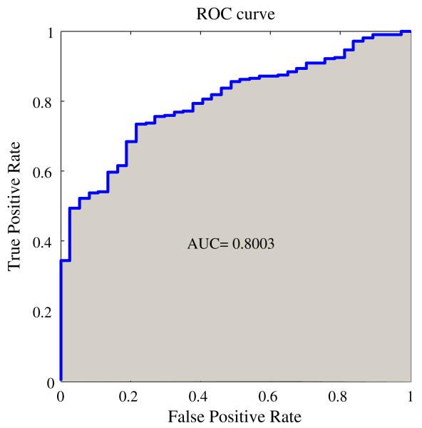
The ROC curve (Metz 1978) is a graphical representation of the relation between true and false positive predictions for all the possible decision thresholds. In the case of SVM classification, thresholds are defined by the SVM value. More specifically, for each threshold a True Positive Rate (T P R = T P /(T P + F N)) and a False Positive Rate (FP R = FP /(FP + T N)) are calculated. Graphed as coordinate pairs, these measures form the ROC curve. An example ROC curve is depicted in Fig. 1. Once the ROC curve constructed, the “area under the curve” (AUC) is used as a validation metric. A perfect AUC will be equal to one. It can be interpreted as the “probability that a classifier will rank a randomly selected positive sample higher than a randomly chosen negative one” (Fawcett 2006). An AUC value of 0.5 indicates no discriminative ability between samples from different classes, which would be equivalent to flipping a coin to make a decision.

Fig. 1.

An example of ROC curve and corresponding AUC

2.4 Parameter selection strategy for SVM

The optimal parameters C and γ of the SVM Gaussian kernel are the maximizers of the cross-validation metrics described in the previous section. A typical approach consists of constructing a grid and choosing the maximizer out of the discrete set of points. Another approach is to use a global optimization method such as a Genetic Algorithm (Goldberg and Holland 1988) or DIRECT (Björkman and Holmström 1999). Typical ranges of parameters, as chosen in this work, are: C ∈ [2⁻¹⁰, 2¹⁷] and γ ∈ [2⁻²⁵, 2¹⁰]. Within these ranges, the SVM can be a hard or soft classifier and the decision boundary can go from a hyperplane to a highly non-linear hypersurface.

2.5 Confidence interval estimation

In order to obtain a confidence interval for the various validation metrics, bootstrapping can be used (Efron and Tibshirani 1997; Varian 2005). For a dataset of size n, bootstrapping works by uniformly selecting, with replacement, n data points from the pool. The validation metric can be recalculated from these bootstrap samples. This process is repeated for a large number of times to form a distribution of validation metric values. From this distribution, 95% or 99% confidence intervals can be empirically estimated.

3 Methodology

3.1 Manufactured non-separable cases

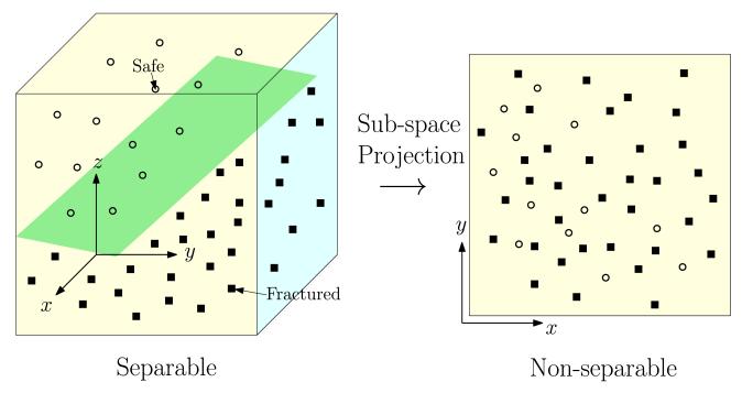
In many engineering or biomedical problems, the data is not separable. This stems from the fact that the data is usually studied in a finite dimensional space which does not account for all the factors that might influence an outcome. For instance, when studying hip fracture data from a cohort of patients, the results are typically reported in a space made of parameters such as age, weight, bone mineral density, etc. Even in the case when this space is high dimensional, the data might still not be separable as the number of dimensions used might still be a fraction of the actual number of factors involved in the occurrence of hip fracture. In other words, non-separable data can be seen as the projection of otherwise separable data onto a space of lower dimensionality. Figure 2 depicts an example in a three dimensional space where the data is separable (separation represented by a plane) and the corresponding projection on a two dimensional space where the data is no longer separable.

Fig. 2.

Manufactured non-separable samples obtained by projection of a separable dataset in a higher dimensional space

Based on these observations, this article proposes to manufacture non-separable cases by projecting the data from a separable space onto its sub-space. The manufactured dataset will exhibit the same type of non-separability encountered in experimental or clinical database. Using this approach, the normally unknown separable case is available and enables the derivation of a “reference” quantity to compare the various validation metrics.

In general, another origin of non-separability also stems from errors in measurements whereby the values of the parameters are not known exactly. By itself, this will contribute to non-separability. Without any loss of generality and for the sake of clarity, this difference will be considered immaterial. Alternatively, the reader can assume that there is no uncertainty on the measured data.

3.1.1 Weighted likelihood

This section introduces a metric which enables the comparison between classifiers constructed with non-separable data. This comparison is made possible by using information from the, usually unknown, model constructed from separable data. The proposed metric is based on the following idea: the non-separable case will produce misclassification. Because of the availability of the classifier with separable data (an approximation of the Bayes classifier (Murty and Devi 2011), it is then possible to find the probability P_i that a misclassified sample x_i belongs to its predicted class.

Gathering and averaging this information for all the misclassified samples, one can form a “weighted likelihood” defined as:

$$\begin{array}{cc}\hfill \overline{{\mathcal{L}}_w}=& \frac{1}{N_{misc}}\sum _{i=1}^{N_{misc}}{w}_i\log \left(P_i\right)\hfill \\ \hfill P_i=& \{\begin{array}{cc}P(-1\mid {\mathrm{x}}_i)\hfill & \text{if}s\left({\mathrm{x}}_i\right)<0\text{and}s\left({\mathrm{x}}_i\right)y_i<0\hfill \\ P(+1\mid {\mathrm{x}}_i)\hfill & \text{if}s\left({\mathrm{x}}_i\right)>0\text{and}s\left({\mathrm{x}}_i\right)y_i<0,\hfill \end{array}\phantom{\}}\hfill \\ \hfill w_i=& \{\begin{array}{cc}1\hfill & \text{if}{y}_i=+1\hfill \\ \frac{N^{+}}{N^{-}}\hfill & \text{if}{y}_i=-1\hfill \end{array}\phantom{\}}\hfill \end{array}$$ (9)

where N_misc is the number of misclassified samples by the SVM constructed in the sub-space, y_i is the actual class of sample x_i and w_i is the weight of for sample x_i. The weights are used for the case where the data is unbalanced.

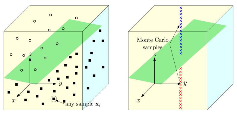
The probability P_i can be efficiently obtained using Monte-Carlo simulations using the SVM from the separable case. Figure 3 provides an example of the methodology in a three dimensional space. For every data point, Monte-Carlo samples are generated along the dimension that is removed to generate a non-separable dataset. In the case of an SVM where the space is split into positive and negative regions, the probability of belonging to the +1 class for any sample x_i can be calculated as:

$$P(+1\mid {\mathrm{x}}_i)=\frac{N_i^{MC+}}{N^{Mc}},i=1,\dots ,N$$ (10)

where x_i is the i^th sample in the sub-space, N^MC is the number of Monte Carlo samples, and $N_i^{MC+}$ represents the number of Monte Carlo samples that are predicted as positive by the SVM constructed with the separable dataset. The corresponding probability of belonging to the −1 class can be calculated as:

$$P(-1\mid {\mathrm{x}}_i)=1-P(+1\mid {\mathrm{x}}_i),i=1,\dots ,N$$ (11)

Fig. 3.

Calculation of the probability of belonging to a class for any sample x_i using Monte Carlo simulation. The sampling is performed based on the variables that were removed to obtain non-separable data

That is, ${\overline{\mathcal{L}}}_w$ is a measure of how correct is the classifier in the sub-space compared to the one with separable samples. The larger algebraic value of the weighted likelihood, the better is the SVM in comparison to the actual separable SVM.

It is also possible to obtain a reference value of the weighted likelihood. This is done by increasing the number of samples until the weighted likelihood converges. The converged value of the likelihood is then considered as the reference value.

4 Results

This section provides results for various SVM classifiers trained and tested using different validation metrics on various dataset configurations. As described in the methodology section, non-separable datasets are generated by projection of a separable case in higher dimension. Sample sets used in this section have different sizes, levels of separability as well as levels of unbalance. The scores for the three validation metrics and the weighted likelihood $\overline{{\mathcal{L}}_w}$ are provided. The SVM model is constructed using a training set which will be used for cross-validation. All the validation metrics are evaluated on a different test set that was not used in the training process. Each result is provided with a corresponding 95% confidence interval.

The following notations are used in this section:

• $\overline{{\mathcal{L}}_w}$: weighted likelihood.

• Ref. $\overline{{\mathcal{L}}_w}$: reference value of weighted likelihood (see Section 3).

• AUC: area under ROC curve.

• Acc: accuracy.

• Bacc: balanced accuracy.

As a test case, we consider the problem of hip fracture prediction. SVM is used as a classifier between fractured and healthy individuals. The data is obtained from a fully parameterized finite element model as described in the following section.

4.1 Fully parameterized finite element model of a femur

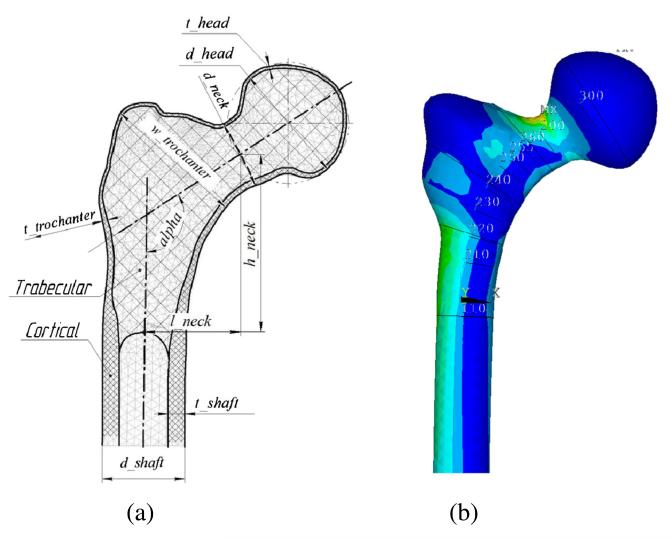
A fully parameterized finite element model of a femur is constructed in ANSYS using ANSYS Parametric Design Language (APDL) (ANSYS 2011). The model parameters are listed in Table 1 and depicted in Fig. 4a. In addition, Fig. 4b depicts an example of contour of principal strain.

Table 1.

Parameters implemented in the finite element model of a femur

Region	Name	Parameter
	Geometric Parameters
Neck	Outer diameter	d_neck
	Thickness of the cortical bone	t_neck
Intertrochanter	Outer width	w_trochanter
	Thickness of the cortical bone	t_trochanter
Shaft	Outer diameter	d_shaft
	Thickness of the cortical bone	t_shaft
	Neck-shaft angle	alpha
	Other Parameters
	Weight	weight
	Young’s modulus	ECortical
	Poisson ratio	ν

Fig. 4.

Fully parameterized finite element model of a femur: a Parameters. b Contour of principal strain. (Max principal strain is around the neck.)

4.2 Sample generation and failure criterion

The data used in the experiments are obtained by sampling three variables: the Young’s modulus of the cortical bone (E_Cortical), the thickness of cortical bone around the neck (T_Neck) and the weight of the individual. Each variable follows a normal distribution with means and standard deviations provided in Table 2. A total of 2000 samples were drawn and evaluated through the finite element model from which stress and strain information can be obtained. In this work, failure (i.e., fracture) is assessed using the maximum principal strain both in tension and compression (Bayraktar et al. 2004). Other measures could be used (Doblaré and García J 2003), however the choice of the measure does not remove any of the generality of the conclusions of the article. The thresholds chosen for the maximum principal strains are 1.04% in compression and 0.73% in tension (Grassi et al. 2012). Based on this failure criterion, samples can be classified into safe (+1) or failed (−1) classes.

Table 2.

Distribution of 3 parameters for sample generation

Parameter	Distribution
E Cortical	N(17.80, 2.10) (GPa)
T Neck	N(1.58, 0.26) (mm)
weight	N(63.96, 15.90) (Kg)

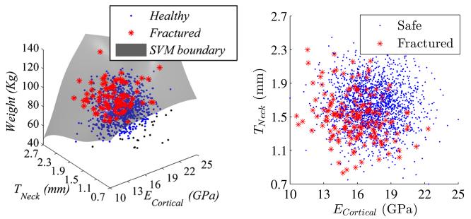
In the three dimensional space, the data is separable because the output of the finite element model is deterministic (Fig. 5). Projection of the three-dimensional samples onto the E_Cortical and T_Neck plane leads to non-separable samples as shown in Fig. 5.

Fig. 5.

3 dimensional SVM with separable data (left). Projection onto the (E_Cortical and T_Neck) space (right)

4.3 Parameter selection using AUC, Acc, and Bacc

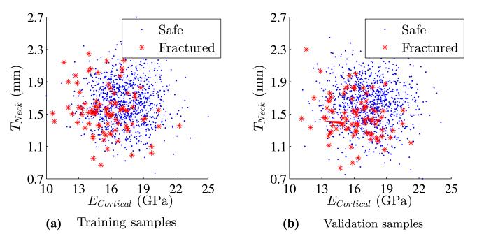
Based on the two-dimensional non-separable samples, the three cross-validation metrics can be used for parameter selection as well as validation of the selected model. For this purpose, the data is randomly split into training and validation sets of equal size as shown in Fig. 6. Parameters of the SVM are selected using k-fold cross-validation based on the training set. The performance of the SVM is carried out on the validation set.

Fig. 6.

Examples of training (a) and validation (b) sample sets

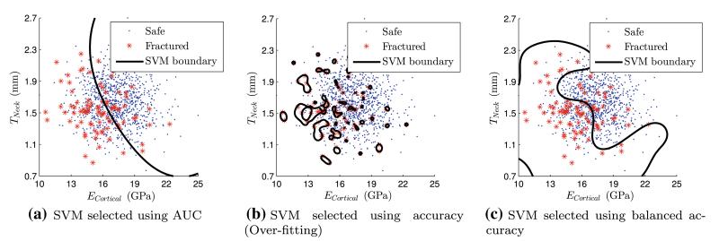
SVMs with highest scores from cross-validation as well as the training sample set are depicted in Fig. 7. The scores for the grid used in the selection of the parameters (C, γ) and the corresponding optima are shown in Fig. 8. It is noteworthy that the SVM selected using the basic accuracy metric leads to “over-fitting” and will have a poor predictive capability.

Fig. 7.

Training samples and SVMs selected based on different validation metrics

Fig. 8.

Maps of validation metrics on a grid along with the corresponding maxima

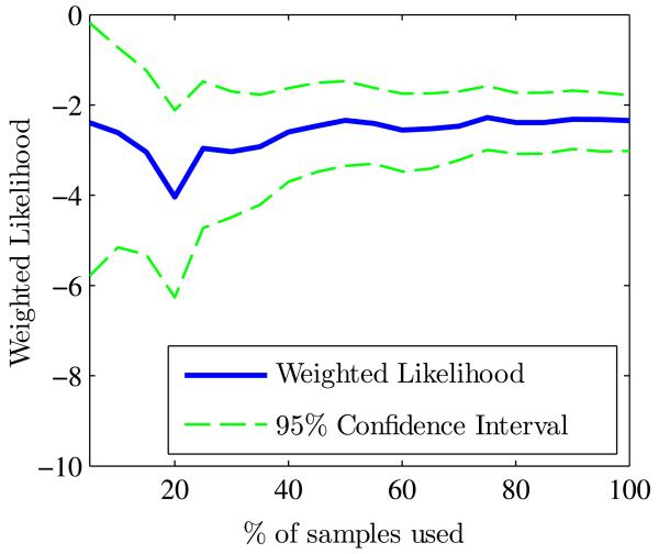
Table 3 provides the results for the weighted likelihood which is compared to the reference value described in Section 3. Figure 9 depicts the convergence of the weighted likelihood as a function of the number of training samples which is used to obtain the reference likelihood value.

Table 3.

Validation metrics (scores) and 95% confidence intervals

SVM selected using:	Score [95% CI]				Difference from Ref. $\overline{{\mathcal{L}}_w}$ *
	AUC	Acc	Bacc	$\overline{{\mathcal{L}}_w}$ [95% CI]
AUC	0.73 [0.68 0.78]	0.68 [0.65 0.71]	0.65 [0.60 0.71]	−3.02 [−4.03 −2.06]	28.78%
Acc	0.58 [0.51 0.64]	0.85 [0.83 0.87]	0.55 [0.51 0.60]	−10.64 [−13.30 −8.16]	353.40%
Bacc	0.67 [0.61 0.73]	0.70 [0.67 0.73]	0.63 [0.57 0.69]	−3.90 [−5.11 −2.77]	66.08%

Reference $\overline{{\mathcal{L}}_w}$ =−2.35 [−3.02, −1.78]

Fig. 9.

Evolution of the weighted likelihood $\overline{{\mathcal{L}}_w}$ and its 95% confidence interval as a function of the number of training samples. The reference $\overline{{\mathcal{L}}_w}$ is the value at convergence

From this point on, this article will not consider accuracy (Acc) metric since it is not suitable (and this is a well-known problem) in the case of unbalanced data.

4.4 Influence of separability, unbalance, and training sample size

This section extends the previous study to different levels of separability, unbalance, and sizes of training sample sets.

4.4.1 Level of separability

In order to create configurations with different levels of separability, the spread of fractured samples in sub-space of E_Cortical and T_Neck was modified. For this purpose, an isoprobabilist transformation between the original normal distributions and new Weibull distributions was used:

$$F({\mathrm{x}}_i\mid a,b)=\Phi \left(\frac{{\mathrm{x}}_i-{\mu }_i}{{\sigma }_i}\right),i=1,2$$ (12)

where F(x_i|a, b) is the cumulative distribution function of Weibull distribution with parameter a and b. φ is the cumulative distribution function of the standard normal distribution. μ_i and σ_i are the empirical mean and standard deviation of variables E_Cortical and T_Neck separately. The parameters of the Weibull distribution were modified to control the spread.

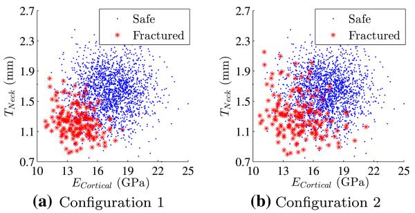
In addition to the original distribution (Fig. 5), two new levels of separability are introduced (Fig. 10 a and b). These three levels of separability will be referred to as Configuration 1,2 and 3. Configuration 3 refers to the original case without transformation.

Fig. 10.

Different sample configurations with two levels of separability

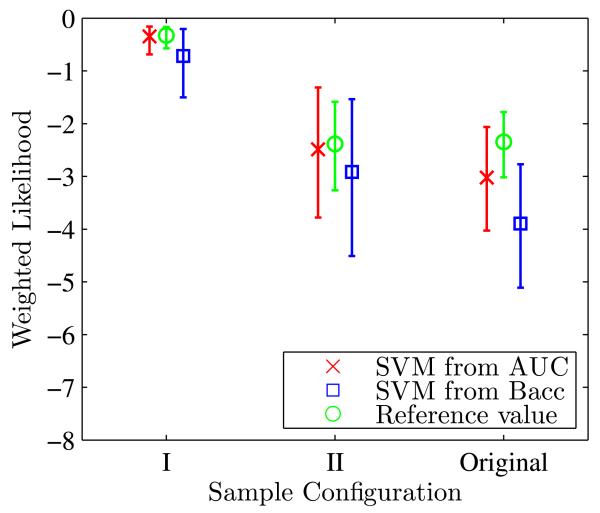
Figure 11 shows the evolution of weighted likelihood as well as its 95% confidence interval for both sample configurations 1 and 2. The evolution is depicted as a function of the number of training samples. Reference values of weighted likelihood for sample configuration 1 & 2 as well as their 95% confidence intervals are given in Tables 4 and 5.

Fig. 11.

Evolution of $\overline{{\mathcal{L}}_w}$ and its 95% confidence interval for the two separability levels as a function of number of training samples

Table 4.

Validation metrics and 95% confidence intervals for level of separability “Configuration 1”

SVM selected using:	Score [95% CI]				Difference from Ref. $\overline{{\mathcal{L}}_w}$ *
	AUC	Acc	Bacc	$\overline{{\mathcal{L}}_w}$ [95% CI]
AUC	0.97 [0.96 0.98]	0.89 [0.87 0.91]	0.93 [0.91 0.95]	−0.35 [−0.69 −0.16]	6.05%
Bacc	0.97 [0.96 0.98]	0.83 [0.81 0.85]	0.90 [0.88 0.92]	−0.72 [−1.50 −0.20]	118.67%

^*Reference $\overline{{\mathcal{L}}_w}$ =−0.33 [−0.57, −0.17]

Table 5.

Validation metrics and 95% confidence intervals for level of separability “Configuration 2”

SVM selected using:	Score [95% CI]				Difference from Ref. $\overline{{\mathcal{L}}_w}$ *
	AUC	Acc	Bacc	$\overline{{\mathcal{L}}_w}$ [95% CI]
AUC	0.92 [0.88 0.94]	0.82 [0.79 0.84]	0.83 [0.79 0.87]	−2.49 [−3.78 −1.31]	4.21%
Bacc	0.91 [0.88 0.94]	0.84 [0.82 0.86]	0.84 [0.80 0.88]	−2.92 [−4.51 −1.54]	22.33%

^*Reference $\overline{{\mathcal{L}}_w}$ =−2.39 [−3.26, −1.58]

Results on sample separability configuration 1 and 2 are listed in Table 4 and 5 separately.

Figure 12 shows that as the samples become more separable, weighted likelihood from the SVM selected based on AUC is closer to the reference value. In addition, its 95% confidence interval is smaller than the SVM selected based on balanced accuracy.

Fig. 12.

Comparison of weighted likelihood between the three levels of separability

4.4.2 Level of unbalance

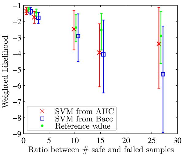
This section studies the change of weighted likelihood and its 95% confidence interval with different levels of unbalance by varying ratios between safe (+1) and failed (−1) classes (Fig. 13). Validation metrics (scores) and relative differences of weighted likelihood to the reference value are listed in Table 6.

Fig. 13.

For separability level “Configuration 2”, study of the influence of unbalance by changing the ratio between safe and failed samples

Table 6.

Performances of SVMs selected using different validation metrics for four levels of unbalance

	SVM selected using:	Score [95% CI]			Difference from Ref. $\overline{{\mathcal{L}}_w}$ *
		AUC	Bacc	$\overline{{\mathcal{L}}_w}$
Case 1	AUC	0.90 [0.87 0.93]	0.84 [0.77 0.90]	−3.40 [−6.17 −1.14]	16.80%
	Bacc	0.90 [0.87 0.94]	0.80 [0.72 0.87]	−5.30 [−8.92 −2.30]	82.20%
Case 2	AUC	0.90 [0.86 0.94]	0.81 [0.75 0.86]	−3.95 [−6.08 −2.16]	55.33%
	Bacc	0.90 [0.86 0.94]	0.83 [0.78 0.88]	−4.06 [−6.46 −1.92]	59.76%
Case 3	AUC	0.90 [0.89 0.92]	0.83 [0.81 0.85]	−1.75 [−2.12 −1.37]	20.76%
	Bacc	0.90 [0.89 0.92]	0.83 [0.80 0.85]	−1.78 [−2.15 −1.45]	23.28%
Case 4	AUC	0.91 [0.90 0.92]	0.8 [0.82 0.85]	−1.36 [−1.58 −1.15]	10.31%
	Bacc	0.89 [0.87 0.91]	0.84 [0.82 0.86]	−1.38 [−1.60 −1.15]	11.52%

¹ Reference $\overline{{\mathcal{L}}_w}$ for Case 1 is −2.91 [−4.63, −1.39].

² Reference $\overline{{\mathcal{L}}_w}$ for Case 2 is −2.54 [−3.79, −1.50].

³ Reference $\overline{{\mathcal{L}}_w}$ for Case 3 is −1.45 [−1.67, −1.24].

⁴ Reference $\overline{{\mathcal{L}}_w}$ for Case 4 is −1.23 [−1.36, −1.12]

Figure 14 shows that as the ratio between safe and failed classes grows larger, the 95% confidence interval of weighted likelihood becomes wider. The use of AUC provides better results than the balanced accuracy: the weighted likelihood is closer to the reference value and also is associated with a tighter confidence interval.

Fig. 14.

Weighted likelihood and its 95% confidence interval for different levels of unbalance

4.4.3 Number of samples

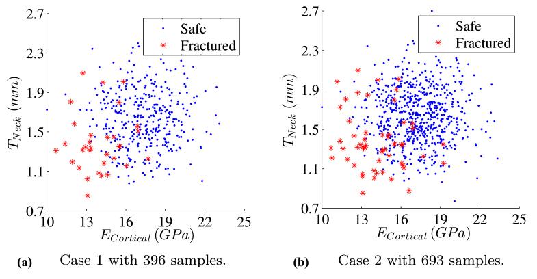
This section studies the influence of the number of samples. The ratio between failure and safe samples is kept constant. Three cases with different sizes of training samples are created as shown in Fig. 15. Case 1 uses 40% of training samples, Case 2 uses 70% of training samples and Case 3 contains all samples available in the training set as shown in Fig. 10b. The size of the test set is constant.

Fig. 15.

Different sizes of training samples used for parameter selection

Results of weighted likelihood and relative difference from the reference value are provided in Table 7. As the size of training samples increases, SVMs selected based on AUC demonstrate again a better performance than the balanced accuracy (see Fig. 16).

Table 7.

Performances of SVMs selected using different metrics on validation set for 3 cases with various sizes of training sets

	SVM selected using:	Score [95% CI]			Difference from Ref. $\overline{{\mathcal{L}}_w}$ *
		AUC	Bacc	$\overline{{\mathcal{L}}_w}$
Case 1	AUC	0.91 [0.88 0.93]	0.83 [0.78 0.87]	−3.55 [−5.30 −2.02]	48.89%
	Bacc	0.84 [0.78 0.89]	0.75 [0.70 0.80]	−3.71 [−5.68 −2.00]	55.60%
Case 2	AUC	0.91 [0.88 0.94]	0.83 [0.79 0.87]	−3.26 [−4.91 −1.83]	36.75%
	Bacc	0.85 [0.80 0.90]	0.76 [0.71 0.81]	−3.51 [−5.37 −1.93]	47.35%
Case 3	AUC	0.91 [0.88 0.94]	0.84 [0.80 0.88]	−2.49 [−3.86 −1.31]	4.35%
	Bacc	0.91 [0.88 0.94]	0.83 [0.79 0.87]	−2.86 [−4.37 −1.53]	20.06%

¹ Reference $\overline{{\mathcal{L}}_w}$ =−2.39 [−3.26, −1.58]

Fig. 16.

Weighted likelihood and its 95% confidence interval for different sizes of training samples

5 Conclusion

This article compared three commonly used validation metrics for the selection of optimal SVM parameters in the case of non-separable and unbalanced data. A systematic study with different levels of separability and levels of unbalance as well as sizes of training samples, were presented. The datasets used were created from a finite element model for the prediction of hip fracture. The results show the advantage of the AUC metric, mostly for case with large degrees of unbalance and non-separability. The next steps of this study will involve higher dimensional problems along with the use of actual clinical data.

References

- ANSYS . ANSYS Parametric Design Language Guide. ANSYS Inc; 2011. [Google Scholar]
- Basudhar A, Missoum S. An improved adaptive sampling scheme for the construction of explicit boundaries. Struct Multidiscip Optim. 2010;42(4):517–529. [Google Scholar]
- Basudhar A, Missoum S, Harrison Sanchez A. Limit state function identification using Support Vector Machines for discontinuous responses and disjoint failure domains. Probabilistic Eng Mech. 2008;23(1):1–11. [Google Scholar]
- Bayraktar H, Morgan E, Niebur G, Morris G, Wong E, Keaveny T. Comparison of the elastic and yield properties of human femoral trabecular and cortical bone tissue. J Biomech. 2004;37(1):27–35. doi: 10.1016/s0021-9290(03)00257-4. [DOI] [PubMed] [Google Scholar]
- Björkman M, Holmström K. Global optimization using the direct algorithm in matlab. 1999. [Google Scholar]
- Brodersen K, Ong CS, Stephan K, Buhmann J. The balanced accuracy and its posterior distribution; 2010 20th International Conference on Pattern Recognition (ICPR); 2010. pp. 3121–3124. doi:10.1109/ICPR.2010.764. [Google Scholar]
- Burges CJ. A tutorial on support vector machines for pattern recognition. Data Min Knowl Discov. 1998;2(2):121–167. [Google Scholar]
- Chang CC, Lin CJ. LIBSVM: a library for support vector machines. ACM Trans Intell Syst Technol. 2011;2:1–27. [Google Scholar]
- Cristianini N, Shawe-Taylor J. An introduction to support vector machines and other kernel-based learning methods. Cambridge university press; 2000. [Google Scholar]
- Doblaré M, García J. On the modelling bone tissue fracture and healing of the bone tissue. Acta Científica Venezolana. 2003;54(1):58–75. [PubMed] [Google Scholar]
- Efron B, Tibshirani R. Improvements on cross-validation: the 632+ bootstrap method. J Am Stat Assoc. 1997;92(438):548–560. [Google Scholar]
- Fawcett T. An introduction to roc analysis. Pattern recogn Lett. 2006;27(8):861–874. [Google Scholar]
- Goldberg DE, Holland JH. Genetic algorithms and machine learning. Mach Learn. 1988;3(2):95–99. [Google Scholar]
- Grassi L, Schileo E, Taddei F, Zani L, Juszczyk M, Cristofolini L, Viceconti M. Accuracy of finite element predictions in sideways load configurations for the proximal human femur. J Biomech. 2012;45(2):394–399. doi: 10.1016/j.jbiomech.2011.10.019. doi:10.1016/j.jbiomech.2011.10.019. [DOI] [PubMed] [Google Scholar]
- Jaakkola T, Haussler D, et al. Exploiting generative models in discriminative classifiers. Adv Neural Inf Proces Syst. 1999:487–493. [Google Scholar]
- Kohavi R. A study of cross-validation and bootstrap for accuracy estimation and model selection; International joint Conference on artificial intelligence, Lawrence Erlbaum Associates Ltd.1995. pp. 1137–1145. [Google Scholar]
- Konig I, Malley J, Pajevic S, Weimar C, Diener H, Ziegler A. Tutorial in biostatistics patient-centered prognosis using learning machines. 2005. [DOI] [PMC free article] [PubMed] [Google Scholar]
- Matthews BW. Comparison of the predicted and observed secondary structure of t4 phage lysozyme. Biochimica et biophysica acta. 1975;405(2):442. doi: 10.1016/0005-2795(75)90109-9. [DOI] [PubMed] [Google Scholar]
- McLachlan GJ, Do KA, Ambroise C. Vol. 422. Wiley-Interscience; 2004. Analyzing microarray gene expression data. [Google Scholar]
- Metz CE. Seminars in nuclear medicine. Vol. 8. Elsevier; 1978. Basic principles of ROC analysis; pp. 283–298. [DOI] [PubMed] [Google Scholar]
- Murty MN, Devi VS. Pattern recognition, An algorithmic approach. Springer; 2011. [Google Scholar]
- Opper M, Winther O. Gaussian processes for classification: mean-field algorithms. Neural Comput. 2000;12(11):2655–2684. doi: 10.1162/089976600300014881. [DOI] [PubMed] [Google Scholar]
- Osuna E, Freund R, Girosi F. Support vector machines. Training and applications. 1997 [Google Scholar]
- Rijsbergen CJV. Information Retrieval. 2nd edn. Butterworth-Heinemann, Newton; 1979. [Google Scholar]
- Tay FE, Cao L. Application of support vector machines in financial time series forecasting. Omega. 2001;29(4):309–317. [Google Scholar]
- Vapnik V. The nature of statistical learning theory. springer; 1999. [DOI] [PubMed] [Google Scholar]
- Vapnik V, Chapelle O. Bounds on error expectation for support vector machines. Neural Comput. 2000;12(9):2013–2036. doi: 10.1162/089976600300015042. [DOI] [PubMed] [Google Scholar]
- Vapnik VN. Statistical learning theory. Wiley; 1998. [DOI] [PubMed] [Google Scholar]
- Varian H. Bootstrap tutorial. Math J. 2005;9(4):768–775. [Google Scholar]
- Yang ZR. Machine learning approaches to bioinformatics. Vol. 4. World Scientific Publishing Company Incorporated; 2010. [Google Scholar]