Pectoral Muscle Detection in Mammograms Using Local Statistical Features

Abstract

Mammography is a primary imaging method for breast cancer diagnosis. It is an important issue to accurately identify and separate pectoral muscles (PM) from breast tissues. Hough-transform-based methods are commonly adopted for PM detection. But their performances are susceptible when PM edges cannot be depicted by straight lines. In this study, we present a new pectoral muscle identification algorithm which utilizes statistical features of pixel responses. First, the Anderson–Darling goodness-of-fit test is used to extract a feature image by assuming non-Gaussianity for PM boundaries. Second, a global weighting scheme based on the location of PM was applied onto the feature image to suppress non-PM regions. From the weighted image, a preliminary set of pectoral muscles boundary components is detected via row-wise peak detection. An iterative procedure based on the edge continuity and orientation is used to determine the final PM boundary. Our results on a public mammogram database were assessed using four performance metrics: the false positive rate, the false negative rate, the Hausdorff distance, and the average distance. Compared to previous studies, our method demonstrates the state-of-art performance in terms of four measures.

Introduction

Mammography is one of the most important imaging methods for breast disease diagnosis [1]. Two common approaches are head-to-foot (craniocaudal, CC) view and angled side (mediolateral oblique, MLO) view. In most MLO view and some CC view mammograms, pectoral muscles (PM) appear as a high-intensity, triangular region in the upper part of the image, which is in the opposite direction of nipple. To avoid misclassification, PM regions have to be removed from breast areas in intensity-based applications such as breast density evaluations [2, 3], lesion identification [4], etc. In other applications such as registration of multiple view mammograms, PM boundaries, together with nipples and breast skin-air borders, can serve as anatomical landmarks. In both scenarios, it is an important issue to accurately identify and separate pectoral muscles from breast tissues [5].

On a typical MLO mammogram, PM can be seen as a triangular area in the top corner, and its boundary can be approximately fitted by a straight line [6]. Based on this observation, various Hough transform (HT)-based methods were developed [7]. In these approaches, PM boundaries are fitted as straight lines. To suppress interference by other tissues, mammograms are often pre-enhanced using canny operator [8] and other filters. The accuracy of HT-based approaches is limited when curvatures of real pectoral muscle boundaries cannot be omitted. For this reason, many modifications have been developed. Yam et al. utilized dynamic programming to fit the curved pectoral edges [9]. Kwok et al. extracted the fine boundary by iteratively searching the edge points around straight line of PM [10]. These methods were sensitive to preliminary line detections and were not reliable on texture edges. Different from the HT-based methods, Zhou et al. applied the shortest path searching algorithm to identify pectoral muscle boundaries, in which the straight line assumption was employed to determine PM orientations [2].

PM detection methods without the straight-line assumption were also developed. Ferrari et al. proposed a Gabor-filter method to detect PM boundaries by locating pixels with opposite phase orientation [11]. Ma et al. proposed two graph-theory-based segmentation methods in conjunction with active contour to segment the pectoral muscles [12]. Camilus et al. developed a graph cut-based segmentation method to detect the pectoral edge and smoothed the edge using Bezier curve [13]. Such methods outperformed the HT method in terms of the false positive (FP) rate, the false negative (FN) rate, and other performance measures. Some studies retrieved PM boundaries from re-quantized version of mammograms. Mustra et al. converted mammograms into 3-bit images and located pectoral muscle boundaries using wavelet decompositions [14]. Similarly, Carvalho et al. reduced mammograms to nine gray levels and detected pectoral muscle boundaries by performing morphological operations at each level [15]. Iglesias and Karssemeijer introduced a different detection method using information of multiple mammograms. The method utilized the statistical information of image sets to improve the accuracy [16].

In this study, we developed a new pectoral muscle boundary detection method which consists of several successive steps. First, the pixel-wise statistical features of mammogram are evaluated using a 2D Anderson–Darling (AD) filter. Next, a weight matrix is then applied on the AD mapping to suppress the non-PM regions. From the resulted AD image, a preliminary boundary set is defined as the row-wise maxima. Finally, the accurate PM boundary is obtained from the set by iteratively searching the candidate curves. To the best of our knowledge, it is the first study that uses the goodness-of-fit style filter for mammography analysis. The method is more sensitive to weak PM edges than common gradient-based detection. Besides, the proposed iterative searching method in the final step has no limits on contour shapes and is more flexible when PM boundaries cannot be well described by straight lines or simple curves.

The rest of the paper is organized as follows: In “Method” section, the proposed method of PM detection is discussed. The experimental results are demonstrated in “Results” section. In “Discussion and Comparison” section, we discuss the performance of proposed method and compare it with existing studies. We conclude our work in “Conclusion” section.

Method

In this section, we explain the proposed algorithm of pectoral muscle detection using weighted AD images. For simplicity, we illustrate the method using MLO view mammograms. The weight matrix and searching rules are developed using the characteristic of MLO images. The method can be applied on CC view mammograms by adjusting the parameters accordingly. For convenience, the proposed method is explained for the left breast mammogram. The right breast mammogram can be processed in the same fashion once it is flipped horizontally. Besides, we further assume that all test mammograms have PM regions.

AD Image Generation Using a Pixel-Wise Discrepancy Measure

Without loss of generality, a pixel o_ij in a mammogram can be treated as a Gaussian random variable that satisfies . In smooth region, the parameters μ_ij, σ²_ij of the pixel can be estimated using its neighbors. The agreement does not held when pixel o_ij is in a non-uniform region where strong local intensity variations exist. In other words, the pixel and its neighbors cannot be well modeled using Gaussian distribution. To measure the discrepancy, we selected the AD test which is suitable for small sample sets. Suppose a sample set contains total m observations of random variable o with a desired distribution F₀(o). Meanwhile, its empirical distribution function can be estimated as F_n(o) = r/m if r of m samples is no larger than o_i. The discrepancy between the empirical distribution and the desired distribution of sample sets can be measured using the goodness-of-fit test statistics [17],

1

where function f₀(o) is the probability density function of F₀(o) and ψ(⋅) is a weight function. Equation (1) is the AD test when ψ(F₀(o)) = [F₀(o)(1 − F₀(o))]^− 1.

The AD metric in Eq. (1) can be further converted into a discrete form

2

where {o_i} are sorted samples, {o₁ < … < o_m}. Replacing F₀(o) as the desired Gaussian distribution, the AD values can be employed directly as measures of unlikeness of set {o_i} to a Gaussian distribution, or “non-Gaussianity” of variable o. It is unlikely that the sample set is from a Gaussian distribution if the corresponding AD value is large. In our study, the AD value of a pixel is calculated using its w × w neighbors. w was set to 11 by trail and error. The AD measure was pixel-wisely applied on a mammogram to generate a 2D AD image.

Enhanced AD Images

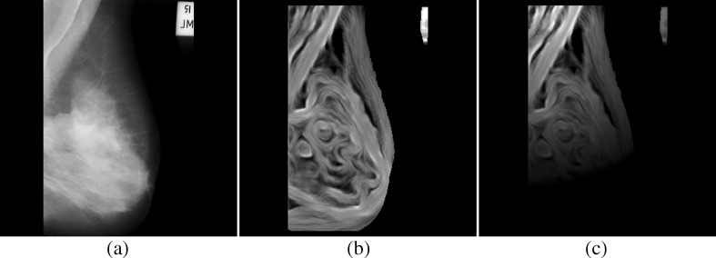
A mammogram is an intensity mapping of X-ray radiation. In Fig. 1a, an example (mdb110) from the mini-MIAS database is demonstrated. In its smooth regions, such as pectoral muscles and mass areas, local pixels have similar values, and the corresponding AD values are relatively small. In non-uniform regions containing PM boundaries or tissue textures, a pixel and its neighbors demonstrate strong intensity variations. The fluctuations are far from the identical Gaussian distribution assumption and lead to much larger AD values than smooth regions. On the AD image, the bright pixels are related to a higher spatial frequency contents in the original mammogram. As can be observed in Fig. 1b, PM boundaries, skin-to-air boundaries, and textures of breast tissues are bright in the AD image. PMs are high-intensity triangular regions on MLO view mammogram and are often obscured by overlapped breast tissues.

Fig. 1.

A mammogram and its AD map (mdb110 from the MIAS database; a original, b AD map, c weighted AD map)

To suppress non-PM regions, a weight matrix H is constructed to modulate the AD image. The coefficients are selected based on the fact that the PM is a high density area on one side of upper part in a typical MLO mammogram.

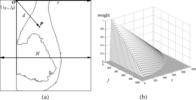
For a typical X-ray breast image shown in Fig. 2a, which denotes the upper left corner of the PM at (i₀, j₀) as the origin O, the weight on a AD pixel at (i, j) is,

3

where d is the Euclidean distance from pixel P to pixel O (i₀, j₀) and r is the distance from (i₀, j₀) to the right side of the image, r = N − i₀. The matrix H has the same size as the AD image. The 3D view of the matrix is plotted in Fig. 2b. The AD pixels are multiplied by the corresponding elements in H to produce the weighted AD image shown in Fig. 1c.

Fig. 2.

Construction of the weight matrix (a weight calculation, b 3D view of weight matrix)

Preliminary Boundary Sets

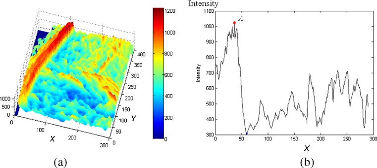
A preliminary boundary is a pixel set containing all row-wise maxima since PM edges usually demonstrate the largest values on the weighted AD images. As the AD map shown in Fig. 3a, the red ridge (maximum values) represents the PM boundary. Given y-axis position, the profile of one row (parallel to x-axis) is shown in Fig. 3b. Peak A represents a point on the PM edge. By locating all peaks row by row, a preliminary boundary set C₀ are obtained. If multiple maximal pixels exist in one row, the average position is selected. Other selections are possible such as the median, the most right, etc. But we found that the average provides the best performance in experiments. Note that the accurate positions of C₀ is w/2 pixels left to the peak because of the diffusion caused by the AD operator.

Fig. 3.

Row-wise peaks on AD map (a AD map of a ROI containing PM, b row-wise profile at y = 300)

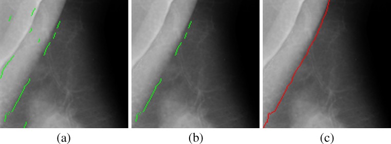
Due to density variations, boundary set C₀ is usually not a continuous curve along a PM boundary. As shown in Fig. 4a, C₀ is a set composed of curve segments and isolated pixels. Note that there is no overlap among segments as their pixels were determined row by row. Besides, components of C₀ often deviate from the actual PM boundary when row-wise maxima are not in PM boundary regions. The preliminary set of the PM boundary has to be further processed, as shown in Fig. 4b, to obtain the accurate representation shown in Fig. 4c.

Fig. 4.

PM boundary detection (a PM boundary set C ₀, b longest sub-boundary, c pectoral boundary C _e)

Final PM Boundary Retrieval

To accurately identify the PM boundary from C₀, we proposed an iterative procedure using prior knowledge on typical left MLO view mammograms: PM boundaries are continuous curves whose directions are from the lower left to the upper right. The boundary features of continuity and orientation are utilized for the detection.

Continuity

Two successive pixels on a continuous curve should be connected. Instead of 8-connectivity in a 3 × 3 neighborhood, 24-connectivety on a 5 × 5 neighborhood is implemented to better capture the local variations on the boundaries. Mathematically, two column-wise successive pixels at (i_a, j) and (i_b, j + 1) are connected if |i_a − i_b| ≤ 2.

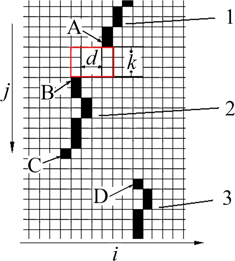
Based on pixel connectivity definition, the connectivity of two boundary segments is also defined. As shown in Fig. 5, the vertical distance is k between end pixel A at (i_a, j) on segment 1 and end point B at (i_b, j + k) on segment 2. Two segments are connected if

4

Fig. 5.

Segment connectivity on boundary set C ₀

In Fig. 5, segments 1 and 2 are connected, while segments 2 and 3 are not connected according to Eq. (4). A “sub-boundary” is a set of all “connected” boundary segments. There are two sub-boundaries in Fig. 5. One is the combination of segments 1 and 2; the other is segment 3.

Orientation

A PM boundary spans from top right to bottom left on a left breast MLO mammogram. The orientation can be adopted to constrain positions of segments in set C₀. For example, two segments 1 and 2 should satisfy the constraint

5

if they are on PM boundary, where (i₁, j₁) and (i₂, j₂) are pixel averages of two segments.

The continuity and orientation constraints are employed alternately to extract a PM boundary from set C₀. Pixels and segments along a sub-boundary are reserved only if they satisfied the two constraints. The missing components are determined by searching the row-wise maxima in the local areas defined by two neighbor elements in the sub-boundary. Such operations are conducted iteratively until a continuous PM boundary curve is retrieved. The detailed procedure to retrieve a PM boundary from C₀ is described as follows:

1. Set i = 0.

2. Scan pixels on C_i and find all sub-boundaries on C_i.

3. Select the longest sub-boundary b^l_i from C_i as the candidate boundary. If b^l_i is the unique element of set C_i, select b^l_i as the final PM boundary and stop the iteration.

   Note that b^l_i might be a discontinuous curve composed of multiple segments and pixels.

4. Find the missing pixels of b^l_i and generate boundary set C_i + 1 which is composed of b^l_i and all its missing pixels.

   A missing region is a rectangular region defined by positions of the last pixel of a segment and the first pixel on the successive segment. For example, a “missing region” is defined in Fig. 5 by pixel A, the last pixel of segment 1, and pixel B, which is the first pixel of segment 2. The missing pixels are detected as the local row-wise maxima in the regions.

5. i = i + 1, return to step 2.

The procedure is a fully automatic operation. Once the preliminary boundary set C₀ is given, a continuous PM curve will be identified by iteratively executing steps 1–5.

Results

In this section, we applied the proposed algorithm on MLO-view mammograms in the mini-MIAS database [18]. The image resolutions are 1,024 × 1,024 with 200-μm-pixel pitches. To simplify the processing, all right breast mammograms (with odd filename numbers) were flipped horizontally such that all images face the same (left) direction. The lateralities could also be detected by analyzing the horizontal intensity distributions.

Performance Measures

The automatic detected results are compared with the set (T2) of manual boundaries depicted by an experienced radiologist (SP). The FP rate is the percentage of detected pixels outside the manually demarcated PM region, while the FN rate is the percentage of non-detected pixels in the manually demarcated PM regions. The other two measures are the average distance and Hausdorff distance.

The Average Distance d_ave

The average distance d_ave between two curves is the average distance d_pc of all pixels on one curve to another curve. d_ave is always a positive value. The smaller the value of d_ave, the better match between the two curves. The value approaches zero when the two curves are overlapped exactly.

The Hausdorff Distance d_Hau

The Hausdorff distance is a measure between two point sets from each other [19]. It reflects the resemblance between two objects. The measure is the maximum distance of points in one set to another set and defined as,

Performance on the MIAS Dataset

All mammograms were manually pre-screened to exclude mammograms without PM. For 318 mammograms with PM, the values of four performance metrics were calculated. Overall statistics are shown in the third column of Table 1. The average FP rate is 2.32 %, and the average FN rate is 3.81 %. To compare with previous studies, two distance measures are calculated in millimeters. The average and standard deviation of d_ave values are 2.12 ± 1.83 mm, and the average and standard deviation of d_Hau values are 3.27 ± 4.57 mm. We also executed an alternative method in which the AD image is replaced by the gradient image that is computed using the Sobel operator. The results are listed on the right side of Table 1. Using the same searching approach, the two methods obtained the similar results when the PM boundaries are clear and strong. However, the gradient method failed to locate the boundaries when the PM regions are obscured.

Table 1.

Agreement of computerized detection with the manual reference

	Measures	AD	Gradient
FP	Average	2.32 %	3.34 %
	Standard deviation	3.45 %	4.17 %
FN	Average	3.81 %	4.57 %
	Standard deviation	5.21 %	4.79 %
d ave	Average	2.12 mm	3.57
	Standard deviation	1.83 mm	3.35
d Hau	Average	3.47 mm	4.15
	Standard deviation	4.57 mm	5.14

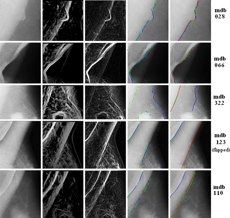
Visual examples are demonstrated in Fig. 6. In this figure, the regional of interests (ROIs) of four mammograms with different PM patterns are shown row by row. Original and processed images are listed in multiple columns. From left to right, they are the originals, AD images, gradient images, the PM boundary sets by AD (in green) and gradient (in blue), and the final results with manual references (in red).

Fig. 6.

PM boundary detection on multiple mammograms (from left to right: originals, AD images, edge image, boundary set C ₀, and detected boundary; red reference, blue edged-based results, green AD-based results)

The first two rows are images of mdb028 and mdb066. PM regions are distinguished from the background clearly on these two examples. Although the contours are not the straight lines, both AD- and gradient-based searching methods retrieved the contours with high accuracy. The third row is from mdb322, on which the PM boundary is obscured. For such cases, the AD method is more robust to retrieve the correct PM boundaries than the gradient method. The last two rows demonstrate the cases with folded PMs (mdb123 and mdb110). On such mammograms, multiple contours exist in the PM regions. The performance of the proposed method is sensitive. For mdb110, the AD detected contour is close to the reference. However, the result of mdb123 is far to the manual result.

Discussion and Comparison

Our method utilizes both regional and global information to detect the pectoral muscle on MLO view mammograms. The local operations include pixel-wise AD measure and the connectivity detection on accurate PM boundary. To enhance the PM regions, a global operation of weight matrices is applied on AD images. Prior knowledge of pectoral boundary locations and orientations are also adopted to retrieve the accurate results.

We evaluated the observer variability in this study. Besides the reference boundary set T2 using in “Performance on the MIAS Dataset” section, a subset of mammograms (100 images) were independently annotated by two persons in our previous study conducted 8 months earlier: T1 by the same radiologist SP and J1 by the second author who was trained by SP. The three manual data sets T1, T2, and J1 were used to evaluate the inter-observer and intra-observer variability in PM boundary detection. Table 2 shows the agreements between manual boundaries and between the computer detected boundaries (AD) and manual references. The values in the table are difference between every two sets listed in terms of four measures. The results in row (J1, T1) and row (J1, T2) show the inter-observer variability in terms of averages and standard deviations of the four metrics. The results for intro-observer variability evaluation are shown in row (T1, T2). Three sets of comparison between the computer method and the manual works are also shown, which are (AD, J1), (AD, T1), and (AD, T2).

Table 2.

Effects of observer variability on pectoral muscle boundary identification using AD-based approach

		FP (%)	FN (%)	d ave (mm)	d Hau (mm)
(J1, T1)	Mean	1.98	3.41	1.21	3.62
	Standard deviation	3.31	4.86	2.27	5.43
(J1, T2)	Mean	1.82	3.21	1.33	3.79
	Standard deviation	3.40	5.02	1.99	5.56
(T1, T2)	Mean	2.02	3.58	0.98	3.87
	Standard deviation	2.72	5.27	2.18	5.32
(AD, J1)	Mean	2.12	3.78	1.67	4.33
	Standard deviation	3.42	5.18	1.87	4.83
(AD, T1)	Mean	2.21	3.67	1.46	4.17
	Standard deviation	3.13	4.79	1.95	5.48
(AD, T2)	Mean	2.32	3.81	2.12	3.47
	Standard deviation	3.45	5.21	1.83	4.57

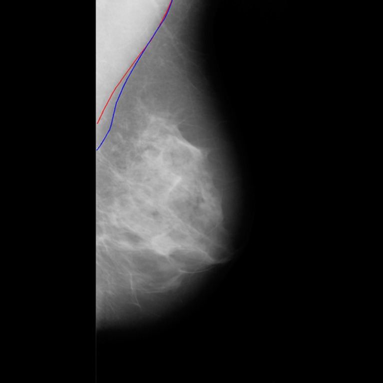
From the observer variability analysis shown in Table 2, no essential difference was found from the comparisons of the automatic and three manual references in terms of four performance measures. For example, the average Hausdorff distance between two manual sets (J1, T1) is 3.62 mm, while the value between the automatic set and one manual set(AD, T2) is 3.47 mm. Errors of detected PM using our method are not significantly larger than the intra/inter-observer variabilities between manual references. When PM edge is weak, the manual contours between two observations are far from consistency due to the subjective judgment on subtle boundaries. This is the major cause of the manual disagreement. For example, two different contours are shown in Fig. 7. They were manually labeled by two observers (T1 and J1) for the same PM region. In such case, the deviations of AD detected contours to the manual references are in the same scales of difference between the manuals. Similar results are also reported in [2].

Fig. 7.

Manually labeled PM boundaries of mdb128 (blue T1; red J1)

To further evaluate the effects of reference variabilities on the performance of the proposed method, paired t tests were performed on pairs of three automatic manual comparisons in terms of four metrics. The two-tailed p values are also shown in Table 3. At the significant level of 0.05, the differences among AD and manual pairs are not statistically significant. However, the statement is not true for AD and gradient results shown in the last row.

Table 3.

The p values from the t test on pairs of observations

	FP	FN	d ave	d Hau
(AD, J1) vs. (AD, T1)	0.141	0.415	0.121	0.132
(AD, J1) vs. (AD, T2)	0.210	0.531	0.071	0.382
(AD, T1) vs. (AD, T2)	0.108	0.342	0.063	0.247
(AD, T2) vs. (gradient, T2)	0.045	0.141	0.031	0.043

The performance of the proposed method is compared with the state-of-the-art studies shown in Table 4. In the table, “Hough” and “Gabor” are two methods in [11], and “AP” and “MST” are methods in [12]. The other three methods are “Radon” [8], “TFO” [2], and “Atlas” [16]. The last one “AD” represents the proposed method. The values from the referred literatures are listed in terms of four measures. Values not provided are labeled as missing data. The average FN rate of 3.81 % using our method is close to that of the TFO method and lower than all others. In terms of the Hausdorff distance, our AD-based method is equivalent to the TFO method but superior to others. Overall, the proposed method demonstrates good performance for PM boundary detection on MLO view mammograms.

Table 4.

Comparison with existing methods from references (“AD” is the proposed method)

Methods	FP (%)	FN (%)	d ave (mm)	d Hau (mm)
Hough [11]	1.98 ± 6.09	25.19 ± 19.14	–	7.08 ± 5.26
Gabor [11]	0.58 ± 4.11	5.77 ± 4.83	–	3.84 ± 1.73
AP [12]	3.71	5.95	–	–
MST [12]	2.55	11.68	–	–
Radon [8]	8.99 ± 38.72	9.13 ± 11.87	–	12.45 ± 22.96
TFO [2]	2.33 ± 3.10	2.88 ± 3.19	1.12 ± 0.82	3.45 ± 2.16
Atlas [16]	2.23	6.62	7.60	23.96
Proposed	2.32 ± 3.45	3.81 ± 5.21	2.12 ± 1.83	3.47 ± 4.57

The proposed method is composed of two major steps: the AD processing and the iterative contour searching. To the best of our knowledge, our method is the first approach that uses AD Gaussianity test for pectoral muscle enhancement in mammograms. Compare with common gradient-based approaches, the AD method is more robust on cases with weak PM edges. To identify the accurate PM boundary, we developed an iterative method to determine local maxima on AD images. The method has no assumption on contour shape (e.g., straight line) and is more flexible when the PM regions have complicated boundaries. The proposed method is based on the assumption that a mammogram has one strong PM edge. It cannot determine if a result is the true PM edge when a mammogram has no PM or multiple PM edges (e.g., folded PM).

Conclusion

We have proposed a novel method to detect pectoral muscles on mammograms using the local non-Gaussianity measure. The accurate PM boundary is identified using an iterative procedure which utilizes a prior knowledge of PM positions and orientations. Experiments on a mini-MIAS dataset demonstrate the competitive performance of the proposed method. The method also provides the flexibility for PM detections on other applications. The appearances of pectoral muscles on CC view mammograms are different. On these images, the PMs are usually on one side of images. The weight function in Eq. (3) can be changed to suppress the non-PM region on the other side. Similarly, the searching rules should also adjust according to the PM geometries on CC view mammograms. An extension of the proposed method to CC view images is an interesting topic to be considered.

References

- 1.Tang J, Rangayyan RM, Xu J, Naqa IE, Yang Y. Computer-aided detection and diagnosis of breast cancer with mammography: recent advances. IEEE Trans Inf Technol Biomed. 2009;13:236–251. doi: 10.1109/TITB.2008.2009441. [DOI] [PubMed] [Google Scholar]
- 2.Zhou C, et al. Computerized image analysis: texture-field orientation method for pectoral muscle identification on MLO-view mammograms. Med Phys. 2010;37:2289–2299. doi: 10.1118/1.3395576. [DOI] [PMC free article] [PubMed] [Google Scholar]
- 3.Liu L, Wang J, He K: Breast density classification using histogram moments of multiple resolution mammograms. In: 3rd International Conference on Biomedical Engineering and Informatics (BMEI), 2010, pp 146–149
- 4.Moayedi F, Azimifar Z, Boostani R, Katebi S. Contourlet-based mammography mass classification using the SVM family. Comput Biol Med. 2010;40:373–383. doi: 10.1016/j.compbiomed.2009.12.006. [DOI] [PubMed] [Google Scholar]
- 5.Ganesan K, Acharya UR, Chua KC, Min LC, Abraham KT. Pectoral muscle segmentation: a review. Comput Methods Prog Biomed. 2013;110:48–57. doi: 10.1016/j.cmpb.2012.10.020. [DOI] [PubMed] [Google Scholar]
- 6.Chakraborty J, Mukhopadhyay S, Singla V, Khandelwal N, Bhattacharyya P. Automatic detection of pectoral muscle using average gradient and shape based feature. J Digit Imaging. 2012;25:387–399. doi: 10.1007/s10278-011-9421-y. [DOI] [PMC free article] [PubMed] [Google Scholar]
- 7.Karssemeijer N. Automated classification of parenchymal patterns in mammograms. Phys Med Biol. 1998;43:365–389. doi: 10.1088/0031-9155/43/2/011. [DOI] [PubMed] [Google Scholar]
- 8.Kinoshita S, Azevedo-Marques P, Pereira R, Jr, Rodrigues J, Rangayyan R. Radon-domain detection of the nipple and the pectoral muscle in mammograms. J Digit Imaging. 2008;21:37–49. doi: 10.1007/s10278-007-9035-6. [DOI] [PMC free article] [PubMed] [Google Scholar]
- 9.Yam M, et al. Three-dimensional reconstruction of microcalcification clusters from two mammographic views. IEEE Trans Med Imaging. 2001;20:479–489. doi: 10.1109/42.929614. [DOI] [PubMed] [Google Scholar]
- 10.Kwok SM, Chandrasekhar R, Attikiouzel Y, Rickard MT. Automatic pectoral muscle segmentation on mediolateral oblique view mammograms. IEEE Trans Med Imaging. 2004;23:1129–1140. doi: 10.1109/TMI.2004.830529. [DOI] [PubMed] [Google Scholar]
- 11.Ferrari R, Rangayyan R, Desautels J, Borges R, Frere A. Automatic identification of the pectoral muscle in mammograms. IEEE Trans Med Imaging. 2004;23:232–245. doi: 10.1109/TMI.2003.823062. [DOI] [PubMed] [Google Scholar]
- 12.Ma F, Bajger M, Slavotinek JP, Bottema MJ. Two graph theory based methods for identifying the pectoral muscle in mammograms. Pattern Recogn. 2007;40:2592–2602. doi: 10.1016/j.patcog.2006.12.011. [DOI] [Google Scholar]
- 13.Camilus KS, Govindan V, Sathidevi P. Computer-aided identification of the pectoral muscle in digitized mammograms. J Digit Imaging. 2010;23:562–580. doi: 10.1007/s10278-009-9240-6. [DOI] [PMC free article] [PubMed] [Google Scholar]
- 14.Mustra M, Bozek J, Grgic M: Breast border extraction and pectoral muscle detection using wavelet decomposition. In: EUROCON 2009, 2009, pp 1426–1433
- 15.de Carvalho IM, et al: An automatic method for delineating the pectoral muscle in mammograms. In: IV Latin American Congress on Biomedical Engineering, Bioengineering Solutions for Latin America, Health, 2007, pp 271–275
- 16.Iglesias JE, Karssemeijer N. Robust initial detection of landmarks in film-screen mammograms using multiple FFDM atlases. IEEE Trans Med Imaging. 2009;28:1815–1824. doi: 10.1109/TMI.2009.2025036. [DOI] [PubMed] [Google Scholar]
- 17.Lehmann EEL, Romano JP. Testing statistical hypotheses. 3. New York: Springer; 2005. [Google Scholar]
- 18.Suckling J et al: The mammographic image analysis society digital mammogram database. In: 2nd international workshop on digital mammography, 1994
- 19.Huttenlocher DP, Klanderman GA, Rucklidge WJ. Comparing images using the Hausdorff distance. Pattern Anal Mach Int IEEE Trans. 1993;15:850–863. doi: 10.1109/34.232073. [DOI] [Google Scholar]