Logistic Stick-Breaking Process

Abstract

A logistic stick-breaking process (LSBP) is proposed for non-parametric clustering of general spatially- or temporally-dependent data, imposing the belief that proximate data are more likely to be clustered together. The sticks in the LSBP are realized via multiple logistic regression functions, with shrinkage priors employed to favor contiguous and spatially localized segments. The LSBP is also extended for the simultaneous processing of multiple data sets, yielding a hierarchical logistic stick-breaking process (H-LSBP). The model parameters (atoms) within the H-LSBP are shared across the multiple learning tasks. Efficient variational Bayesian inference is derived, and comparisons are made to related techniques in the literature. Experimental analysis is performed for audio waveforms and images, and it is demonstrated that for segmentation applications the LSBP yields generally homogeneous segments with sharp boundaries.

1. Introduction

One is often interested in clustering data that have associated spatial or temporal coordinates. This problem is relevant in a diverse set of applications, such as climatology, ecology, environmental health, real estate marketing, and image analysis (Banerjee et al., 2003). The available spatial or temporal information may be exploited to help infer patterns, clusters or segments in the data. To simplify the exposition, in the following discussion we focus on exploiting spatial information, although when presenting results we also consider temporal data (Fox et al., 2008).

There have been numerous techniques developed to cluster data, although most of these do not explicitly exploit appended spatial information. One class of state-of-the-art methods employs graphical techniques, such as normalized cuts (Shi and Malik, 2000; Felzenszwalb and Huttenlocher, 2004) and extensions (Zabih and Kolmogorov, 2004). These approaches regard the two-dimensional (2D) data as an undirected weighted graph, and the segmentation is equivalent to finding the minimum cut of the graph, minimizing the between-group disassociation while maximizing the within-group association (Shi and Malik, 2000). Such graph-theoretic methods have attractive computational speed, but do not provide a statistical inference (measure of confidence), and often one must pre-define the total number of segments/clusters. Further, such graphical techniques are not readily extended to the joint analysis of multiple spatially dependent data sets, with this of interest for the simultaneous analysis of multiple images.

To consider clustering in a nonparametric Bayesian manner, the Dirichlet process (DP) (Blackwell and MacQueen, 1973) has been employed widely (Antoniak, 1974; Escobar and West, 1995; Rasmussen, 2000; Beal et al., 2002). Assume we are given N data points, ${\{{\mathbf{y}}_n\}}_{n=1}^N$, with y_n representing a feature vector; each feature vector is assumed drawn from a parametric distribution F(θ_n). For each y_n, the DP mixture model is represented as

$${\mathbf{y}}_n\mid {\mathit{\theta }}_n~F({\mathit{\theta }}_n),{\mathit{\theta }}_n\mid G\stackrel{\mathit{iid}}{\sim }G,G\mid {\alpha }_0,G_0~\text{DP}({\alpha }_0{G}_0),$$

where α₀ is a non-negative precision parameter and G₀ is the base probability measure. Sethuraman (1994) developed an explicit method for constructing a draw G from a DP:

$$G=\sum _{k=1}^{\infty }{\pi }_k{\delta }_{{\mathit{\theta }}_k^{\ast }},{\pi }_k=V_k\prod _{k^{\prime }=1}^{k-1}(1-V_{k^{\prime }}),V_k\stackrel{\mathit{iid}}{\sim }\text{Beta}(1,{\alpha }_0),{\mathit{\theta }}_k^{\ast }\stackrel{\mathit{iid}}{\sim }{G}_0.$$ (1)

The precision parameter α₀ controls the number of sticks that have appreciable weights, with these weights defining the probability that different θ_n share the same “atoms” ${\mathit{\theta }}_k^{\ast }$. Since α₀ plays an important role in defining the number of significant stick weights π_k, we typically place a gamma prior on α₀ to allow the data to inform about its value.

The assumption within the DP that the data are exchangeable is generally inappropriate when one wishes to impose knowledge of spatial information (in which each y_n has an associated spatial location). For example, the data may be represented as ${\{{\mathbf{y}}_n,{\mathbf{s}}_n\}}_{n=1}^N$, in which y_n is again the feature vector and s_n represents the spatial location of y_n. Provided with such spatial information, one may wish to explicitly impose the belief that proximate data are more likely to be clustered together.

The spatial location s_n may be readily considered as an appended feature, and the modified feature vectors (data) may then be analyzed via traditional clustering algorithms, like those discussed above. For example, the spatial coordinate has been considered explicitly in recent topic models (Cao and Li, 2007; Wang and Grimson, 2007; Gomes et al., 2008) when applied in image analysis. These previous studies seek to cluster visual words, with such clustering encouraged if the features are spatially proximate. However, these methods may produce spurious clusters that are introduced to better characterize the spatial data likelihood instead of the likelihood of the features conditionally on spatial location (Park and Dunson, 2009). In addition, such approaches require a model for the spatial locations, which is not statistically coherent as these locations are typically fixed by design, and there may be additional computational burden for this extra component.

To address these challenges, and impose spatial information more explicitly, researchers have recently modified the DP construction to manifest spatial-location dependent stick weights. The work of Duan et al. (2007) recently introduced a framework in terms of a hierarchy of Gaussian processes, in which the spatially dependent construction is obtained by thresholding K latent Gaussian processes (GPs); while this is a powerful construction, the use of GPs presents computational challenges (Sudderth and Jordan, 2008). To simplify the model structure, the Dirichlet labeling process (Petrone et al., 2009) has been proposed, in which one thresholds only one latent Gaussian process to regulate spatial dependence. However, the model inference, performed with Markov chain Monte Carlo (MCMC), is inefficient for many large-scale applications. Similar issues are also true for work that has combined the Dirichlet process with a Markov random field (MRF) constraint (Orbanz and Buhmann, 2008).

As an alternative to the above approaches, a kernel stick-breaking process (KSBP) has been proposed (Dunson and Park, 2007), imposing that clustering is more probable if two feature vectors are close in a prescribed (general) space, which may be associated explicitly with spatial position for image processing applications (An et al., 2008). With the KSBP, rather than assuming exchangeable data, the G in (1) becomes a function of spatial location:

$$\begin{array}{c}{G}_{\mathbf{s}}=\sum _{k=1}^{\infty }{\pi }_k(\mathbf{s};V_k,{\mathrm{\Gamma }}_k,\psi ){\delta }_{{\mathit{\theta }}_k^{\ast }},\\ {\pi }_k(\mathbf{s};V_k,{\mathrm{\Gamma }}_k,\psi )=V_{k}K(\mathbf{s},{\mathrm{\Gamma }}_k;\psi )\prod _{k^{\prime }=1}^{k-1}[1-V_{k^{\prime }}K(\mathbf{s},{\mathrm{\Gamma }}_{k^{\prime }};\psi )],\\ V_k~\text{Beta}(1,{\alpha }_0),{\mathit{\theta }}_k^{\ast }~G_0,{\mathrm{\Gamma }}_k~H_0,\end{array}$$ (2)

where K(s, Γ_k; ψ) represents a kernel distance between the feature-vector spatial coordinate s and a local basis location Γ_k associated with the kth stick. As demonstrated when presenting results, the KSBP generally does not yield smooth segments with sharp boundaries.

Instead of thresholding K latent Gaussian processes (Duan et al., 2007) to assign a feature vector to a particular parameter, we introduce a novel non-parametric spatially dependent prior, called the logistic stick-breaking process (LSBP), to impose that it is probable that proximate feature vectors are assigned to the same parameter. The new model is constructed based on a hierarchy of spatial logistic regressions, with sparseness-promoting priors on the regression coefficients. With this relatively simple model form, inference is performed efficiently with variational Bayesian analysis (Beal, 2003), allowing consideration of large-scale problems. Further, for reasons discussed below, this model favors contiguous segments with sharp boundaries, of interest in many applications. The model developed in the paper (Chung and Dunson, 2009), based on a probit stick-breaking process, is most closely related to the proposed framework; the relationships between LSBP and the model (Chung and Dunson, 2009) are discussed in detail below.

In addition to exploiting spatial information when performing clustering, there has also been recent research on the simultaneous analysis of multiple tasks. This is motivated by the idea that multiple related tasks are likely to share the same or similar attributes (Caruana, 1997; An et al., 2008; Pantofaru et al., 2008). Exploiting the information contained in multiple data sets (“tasks”), model-parameter estimation may be improved (Teh et al., 2005; Pantofaru et al., 2008; Sudderth and Jordan, 2008). Therefore, it is desirable to employ multi-task learning when processing multiple spatially-dependent data (e.g., images), this representing a second focus of this paper.

Motivated by previous multi-task research (Teh et al., 2005; An et al., 2008), we consider the problem of simultaneously processing multiple spatially-dependent data sets. A separate LSBP prior is employed for each of the tasks, and all LSBPs share the same base measure, which is drawn from a DP. Hence, a “library” of model parameters—atoms—is shared across all tasks. This construction is related to the hierarchical Dirichlet process (HDP) (Teh et al., 2005), and is referred to here as a hierarchical logistic stick-breaking process (H-LSBP).

We present example results on two distinct problem classes, underscoring the general utility of the proposed approach. In the first example we consider segmentation of multi-person spoken audio data. In the second application we employ the H-LSBP to simultaneously segment multiple images. In addition to inferring a segmentation of each image, the framework allows sorting and searching among the images.

The remainder of the paper is organized as follows. In Section 2 we introduce the logistic stick-breaking process (LSBP) and discuss its connections with other models. We extend the model to the hierarchical LSBP (H-LSBP) in Section 3. For both the LSBP and H-LSBP, inference is performed via variational Bayesian analysis, as discussed in Section 4. Experimental results are presented in Section 5, with conclusions and future work discussed in Section 6.

2. Logistic Stick-breaking Process (LSBP)

We first consider spatially constrained clustering for a single data set (task). Assume N sample points {D_n}_n=1,N, where D_n = (y_n, s_n), with y_n representing the nth feature vector and s_n its associated spatial location. We draw a set of candidate model parameters, and the probability that a particular space-dependent data sample employs a particular model parameter is defined by a spatially-dependent stick-breaking process, represented by a kernel-based logistic-regression.

2.1 Model Specifications

Assume an infinite set of model parameters ${\{{\mathit{\theta }}_k^{\ast }\}}_{k=1}^{\infty }$. Each observation y_n is drawn from a parametric distribution F(θ_n), with ${\mathit{\theta }}_n\in {\{{\mathit{\theta }}_k^{\ast }\}}_{k=1}^{\infty }$. To indicate which parameter in ${\{{\mathit{\theta }}_k^{\ast }\}}_{k=1}^{\infty }$ is associated with the nth sample, a set of indicator variables Z_n = {z_n1, z_n2, …, z_n∞} are introduced for each D_n, and all the indicator variables are equal to zero or one. Given Z_n, data D_n is associated with parameter ${\mathit{\theta }}_k^{\ast }$ if z_nk = 1 and z_nk̂ = 0 for k̂ < k.

The Z_n are drawn from a spatially dependent density function, encouraging that proximate D_n will have similar Z_n, thereby encouraging spatial contiguity. This may be viewed in terms of a spatially dependent stick-breaking process. Specifically, let p_k(s_n) define the probability that z_nk = 1, with 1 − p_k(s_n) representing the probability that z_nk = 0; the spatial dependence of these density functions is made explicit via s_n. The probability that the kth parameter is selected in the above model is ${\pi }_k({\mathbf{s}}_n)=p_k({\mathbf{s}}_n){\prod }_{\widehat{k}=1}^{k-1}[1-p_{\widehat{k}}({\mathbf{s}}_n)]$, which is of the same form as a stick-breaking process (Ishwaran and James, 2001) but extends to a spatially dependent mixture model, represented as

$$G_{{\mathbf{s}}_n}=\sum _{k=1}^{\infty }{\pi }_k({\mathbf{s}}_n){\delta }_{{\mathit{\theta }}_k^{\ast }},{\pi }_k({\mathbf{s}}_n)=p_k({\mathbf{s}}_n)\prod _{\widehat{k}=1}^{k-1}[1-p_{\widehat{k}}({\mathbf{s}}_n)].$$

Here each p_k(s_n) is defined in terms of a logistic link function (other link functions may also be employed, such as a probit). Specifically, we consider N_c discrete spatial locations ${\{{\widehat{\mathbf{s}}}_i\}}_{i=1}^{N_c}$ within the domain of the data (e.g., the locations of the samples in D_n). To allow the weights of the different mixture components to vary flexibly with spatial location, we propose a kernel logistic regression for each break of the stick, with

$$log\left(\frac{p_k({\mathbf{s}}_n)}{1-p_k({\mathbf{s}}_n)}\right)=g_k({\mathbf{s}}_n)=\sum _{i=1}^{N_c}{w}_{ki}K({\mathbf{s}}_n,{\widehat{\mathbf{s}}}_i;{\psi }_k)+w_{k0},$$ (3)

where g_k(s_n) is the linear predictor in the logistic regression model for the kth break and position s_n, and

$$K({\mathbf{s}}_n,{\widehat{\mathbf{s}}}_i;{\psi }_k)=exp\left[-\frac{{\left|\right|{\mathbf{s}}_n-{\widehat{\mathbf{s}}}_i\left|\right|}^2}{{\psi }_k}\right]$$

is a Gaussian kernel measuring closeness of locations s_n and ŝ_i, as in a radial basis function model (alternative kernel functions may be defined). The kernel basis coefficients are represented as W_k = [w_k0, w_k1, …, w_kNc]′. A sparseness-promoting prior is chosen for the components of W_k, such that only a relatively small set of w_ki will have non-zero (or significant) amplitudes; those spatial regions for which the associated amplitudes are non-zero correspond to regions for which a particular model parameter is expected to dominate in the segmentation (this is similar to the KSBP in (2), which also has spatially localized kernels). The indicator variables controlling allocation to components are then drawn from

$$z_{nk}~\text{Bernoulli}[\sigma (g_k({\mathbf{s}}_n))],$$

where σ(g) = 1/[1 + exp(−g)] is the inverse of the logit link in (3).

There are many ways that such sparseness promotion may be constituted, and we have considered two. As one choice, one may employ a hierarchical Student-t prior as applied in the relevance vector machine (Tipping, 2001; Bishop and Tipping, 2000; Bishop and Svensén, 2003):

$$w_{ki}~N(w_{ki}\mid 0,{\lambda }_{ki}^{-1})\text{Gamma}({\lambda }_{ki}\mid a_0,b_0),$$

where shrinkage is encouraged with a₀ = b₀ = 10⁻⁶ (Tipping, 2001). Alternatively, one may consider a “spike-and-slab” prior (Ishwaran and Rao, 2005). Specifically,

$$w_{ki}~{\nu }_k\mathcal{N}(0,{\lambda }_k^{-1})+(1-{\nu }_k){\delta }_0,{\nu }_k~\text{Beta}({\nu }_k\mid c_0,d_0).$$

The expression δ₀ represents a unit point measure concentrated at zero. The parameters (c₀, d₀) are set such that ν_k is encouraged to be close to zero (or we simply fix ${\nu }_k=\frac{c_0}{c_0+d_0}$), enforcing sparseness in w_k; the parameter λ_k is again drawn from a gamma prior, with hyperparameters set to allow a possibly large range in the non-zero values of w_ki, and therefore these are not set as in the Student-t representation. The advantage of the latter model is that it explicitly imposes that many of the components of w_k are exactly zero, while the Student-t construction imposes that many of the coefficients are close to zero. In our numerical experiments on waveform and image segmentation, we have employed the Student-t construction.

Note that parameter ${\mathit{\theta }}_k^{\ast }$ is associated with an s-dependent function g_k(s), and there are K − 1 such functions. The model is constructed such that within a contiguous spatial/temporal region, a particular parameter ${\mathit{\theta }}_k^{\ast }$ is selected, with these model parameters used to generate the observed data.

There are two key components of the LSBP construction: (i) sparseness promotion on the w_ki, and (ii) the use of a logistic link function to define space-dependent stick weights. As discussed further in Section 2.2, these concepts are motivated by the idea of making a particular space-dependent LSBP stick weight ${\pi }_k(\mathit{s})=\sigma (g_k(\mathit{s})){\prod }_{k^{\prime }<k}[1-g_k^{\prime }(\mathit{s})]$ near one within a localized region in space (motivating the sparseness prior on the weights), while also yielding contiguous segments with sharp boundaries (manifested via the logistic).

It is desirable to allow flexibility in the kernel parameter ψ, as this will influence the size of segments that are encouraged (discussed further below). Hence, for each k we draw

$${\psi }_k={\psi }_{r_k}^{\ast },r_k~\text{Mult}(1/\tau ,\dots ,1/\tau ),$$

with ${\mathbf{\Psi }}^{\ast }={\{{\psi }_j^{\ast }\}}_{j=1}^{\tau }$ a library of possible kernel-size parameters; r_k is an index for the one non-zero component of a single draw from Mult(1/τ,…,1/τ). We employ a discrete dictionary of kernel sizes Ψ^* because there is not a conjugate prior for imposition of a continuous distribution of kernel parameters (this is discussed further in Section 4). A draw from this hierarchical prior is denoted concisely as G_s ~ LSBP(H, a₀, b₀, Ψ*), where it is assumed that we are using the Student-t prior for weights {w_k}_k=1,K−1, with a similar representation used for a spike-and-slab prior; note that G_s is defined simultaneously for all spatial locations. The model parameters ${\{{\mathit{\theta }}_k^{\ast }\}}_{k=1}^{\infty }$ are assumed drawn from the measure H.

In practice we usually truncate the LSBP to K sticks, as in a truncated stick-breaking process (Ishwaran and James, 2001). With a truncation level K specified, if z_nk = 0 for all k = 1, …, K − 1, then z_nK = 1 so that ${\mathit{\theta }}_n={\mathit{\theta }}_K^{\ast }$. The VB analysis yields an approximation to the marginal likelihood of the observed data, which can be used to evaluate the effect of K on the model performance. When presenting results we consider simply setting K to a large value, and also test the model performance with K initialized to different values.

Figure 1 shows the graphical form of the model (using a Student-t sparseness prior), in which Ψ^* represents the discrete set of kernel-width candidates, ψ_k is the kernel width selected for the kth stick, and the prior H takes on different forms depending upon the application. In Figure 1 the 1/τ emphasizes that the candidate kernel widths are selected with uniform probability over the τ candidates in Ψ^*.

Figure 1.

Graphical representation of the LSBP.

2.2 Discussion of LSBP Properties and Relationship to Other Models

The proposed model is motivated by the work (Sudderth and Jordan, 2008), in which multiple draws from a Gaussian process (GP) are employed. Candidate model parameters are associated with each GP draw, and the GP draws serve to constitute a nonparametric gating network, associating particular model parameters with a given spatial position. In the model (Sudderth and Jordan, 2008) the spatial correlation associated with the GP draws induces spatially contiguous segments (a highly spatially correlated gating network), and this may be related to a spatially-dependent stick-breaking process. However, use of the GP produces computational challenges. The proposed LSBP model also manifests multiple space-dependent functions (here g_k(r)), with associated candidate model parameters ${\{{\mathit{\theta }}_k^{\ast }\}}_{k=1,K}$. Further, we constitute a spatially dependent gating network that has a stick-breaking interpretation. However, a different and relatively simple procedure is proposed for favoring spatially contiguous segments with sharp boundaries.

At each location s we have a stick-breaking process, with the probability of selecting model parameters ${\mathit{\theta }}_k^{\ast }$ defined as π_k(s) = σ(g_k(s)) Π_k′<k[1 − σ(g_k′ (s))]. Recall that $g_k(\mathit{s})={\sum }_{i=1}^{N_c}{w}_{ki}K(\mathit{s},{\widehat{\mathit{s}}}_i;{\psi }_k)+w_{k0}$, with sparseness favored for coefficients {w_ik}_i=0,Nc. Considering first g₁(s), note that since most {w_1i}_i=1,Nc are zero or near-zero, the bias w₁₀ controls the stick weight π₁(s) for all s sufficiently distant from those locations ŝ_i with non-zero w_1i. Further, if w_1i ≫ 0, σ(g₁(s)) ≈ 1 for s in the “neighborhood” of the associated location ŝ_i; the neighborhood size is defined by ψ₁. Hence, those {ŝ_i}_{i=1, Nc} with associated large {w_1i}_i=1,Nc define localized regions as a function of s over which parameter ${\mathit{\theta }}_1^{\ast }$ is highly probable, with locality defined by kernel scale parameter ψ₁. For those regions of s for which π₁(s) is not near one, there is appreciable probability 1 − π₁(s) that model parameters ${\{{\mathit{\theta }}_k^{\ast }\}}_{k=2,K}$ may be used.

Continuing the generative process, model parameters ${\mathit{\theta }}_2^{\ast }$ are probable where π₂(s) = σ (g₂(s))[1 − π₁(s)] ≈ 1. The latter occurs in the vicinity of those s that are distant from ŝ_i with large associated w_1i (i.e., where 1 − π₁(s) ≈ 1), while also being near ŝ_i with large w_2i (i.e., where σ(g₂(s)) ≈ 1). We again underscore that w₂₀ impacts π₂(s) for all s.

This process continues for increasing k, and therefore it is probable that as k gets large all or almost all s will be associated with a large stick weight, or a large cumulative sum of stick weights, such that parameters ${\mathit{\theta }}_k^{\ast }$ become improbable for large k and all s.

Key characteristics of this construction are the clipping property of the logistic link function, and the associated fast rise of the logistic. The former imposes that there are contiguous regions (segments) over which the same model parameter has near-unity probability of being used. This encouraging of homogeneous segments is also complemented by sharp segment boundaries, manifested by the fast rise of the logistic. The aforementioned “clipping” property is clearly not distinct to logistic regression. It would apply as well to other binary response link functions, which can be any CDF for a continuous random variable. For example, probit links (Chung and Dunson, 2009) would have the same property, though the logistic has heavier tails than the probit so may have slightly different clipping properties. We have here selected the logistic link function for computational simplicity (it is widely used, for example, in the relevance vector machine Tipping 2001, and we borrow related technology). It is interesting to see how the segmentation realizations differ with the form of link function, with this to be considered in future research.

To give a more-detailed view of the generative process, we consider a one-dimensional example, which in Section 5 will be related to a problem with real data. Specifically, consider a one-dimensional signal with 488 discrete sample points. In this illustrative example N_c = 98, defined by taking every fifth sample point for the underlying signal. We wish to examine the generative process of the LSBP prior, in the absence of data. For this illustration, it is therefore best to use the spike-and-slab construction, since without any data the Student-t construction will with high probability make all w_ki ≈ 0 (when considering data, and evaluating the posterior, a small fraction of these coefficients are pulled away from zero, via the likelihood function, such that the model fits the data; we reconsider this in Section 5). Further, again for illustrative purposes, we here treat {w_k0}_k=1,K as drawn from a separate normal distribution, not from the spike-and-slab prior used for all other components of w_k. This distinct handling of {w_k0}_k=1,K has been found unnecessary when processing data, as the likelihood function again imposes constraints on {w_k0}_k=1,K. Hence this form of the spike-and-slab prior on w_k is simply employed to illuminate the characteristics of LSBP, with model implementation simplifying when considering data.

In Figure 2 we plot representative draws for w_k, g_k(s), σ(g_k(s)) and π_k(s), for the one-dimensional signal of interest. In this illustrative example each ν_k is drawn from Beta(1, 10) to encourage sparseness, and those non-zero coefficients are drawn from (0, λ), with λ fixed to correspond to a standard deviation of 15 (we could also draw each λ_k from a gamma distribution). Each bias term w_k0 is here drawn iid from (0, λ). We see from Figure 2 that the LSBP naturally favors localized segments that have near-unity probability of using the same model parameters. This is a typical draw, where we note that for k ≥ 4 the probability of ${\theta }_k^{\ast }$ being used is near zero. While Figure 2 represents a typical LSBP draw, one could also envision other less-desirable draws. For example, if w₁₀ ≫ 0 then π₁(s) ≈ 1 for all s, implying that the parameters ${\mathit{\theta }}_1^{\ast }$ is used for all s (essentially no segmentation). Other “pathological” draws may be envisioned. Therefore, we underscore that the data, via the likelihood function, clearly influences the posterior strongly, and the pathological draws supported by the prior in the absence of data are given negligible mass in the posterior.

Figure 2.

Example draw from a one-dimensional LSBP, using a spike-and-slab construction for model-parameter sparseness. (a) w_k, (b) g_k(t), (c) σ_k(t), (d) π_k(t)

As further examples, now for two-dimensional signals, Figure 3 considers example draws as a function of the kernel parameter ψ_k. These example draws were manifested via the same process used for the one-dimensional example in Figure 2, now extending s to two dimensions. Figure 3 also shows the dependence of the size of the segments on the kernel parameter ψ_k, which has motivated the learning of ψ_k in a data-dependent manner (based on a finite dictionary of kernel parameters ${\mathbf{\Psi }}^{\ast }={\{{\psi }_j^{\ast }\}}_{j=1}^{\tau }$. The draws in Figure 3 are similar to those manifested by the GP-based construction (Sudderth and Jordan, 2008), motivating the simple model developed here.

Figure 3.

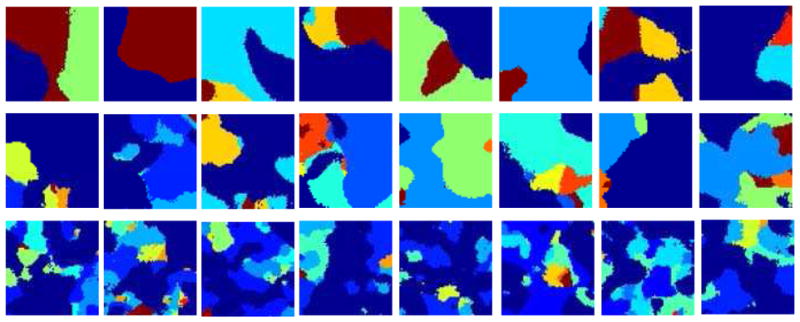
Samples drawn from the spatially dependent LSBP prior, for different (fixed) choices of kernel parameters ψ, applied for each k within the LSBP. In row 1 ψ = 15; in row 2 ψ = 10; and in row 3 ψ = 5. In these examples the spike-and-slab prior has been used to impose sparseness on the coefficients {w_k}_k=1,K−1.

3. Hierarchical LSBP (H-LSBP)

Multi-task learning (MTL) is an inductive transfer framework (Caruana, 1997), with the goal of improving modeling performance by exploiting related information in multiple data sets. We here employ MTL for joint analysis of multiple spatially dependent data sets, yielding a hierarchical logistic stick-breaking process (H-LSBP). This framework models each individual data set (task) with its own LSBP draw, while sharing the same set of model parameters (atoms) across all tasks, in a manner analogous to HDP (Teh et al., 2005). The set of shared model atoms are inferred in the analysis.

The spatially-dependent probability measure for task m, G_m, is drawn from a LSBP with base measure G₀, and G₀ is shared across all M tasks. Further, G₀ is drawn from a Dirichlet process (Blackwell and MacQueen, 1973), and in this manner each task-dependent LSBP shares the same set of discrete atoms. The H-LSBP model is represented as

$$\begin{array}{c}{\mathbf{y}}_{mn}\mid {\mathit{\theta }}_{mn}~F({\mathit{\theta }}_{mn}),{\mathit{\theta }}_{mn}\mid G_m~G_m,\\ G_m\mid \{G_0,a_0,b_0,{\mathbf{\Psi }}^{\ast }\}~\text{LSBP}(G_0,a_0,b_0,{\mathbf{\Psi }}^{\ast }),\\ G_0\mid \gamma ,H~\text{DP}(\gamma H).\end{array}$$

Note that we are assuming a Student-t construction of the sparseness prior within the LSBP, defined by hyperparameters a₀ and b₀.

Assume task m ∈ {1, …, M} has N_m observations, defining the data D_m = {D_m1, …, D_m(Nm)}. We introduce a set of latent indicator variables t_m = {t_m1, …, t_m∞} for each task, with

$$t_{mk}\stackrel{\mathit{iid}}{\sim }\sum _{l=1}^{\infty }{\beta }_l{\delta }_l,k=1,\dots ,\infty ,m=1,\dots ,M,$$ (4)

where β_l corresponds to the lth stick weight of the stick-breaking construction of the DP draw $G_0={\sum }_{l=1}^{\infty }{\beta }_l{\delta }_{{\mathit{\theta }}_l^{\ast }}$. The indicator variables t_mk establish an association between the observations from each task and the atoms ${\{{\mathit{\theta }}_l^{\ast }\}}_{l=1}^{\infty }$ shared globally; hence the atom ${\mathit{\theta }}_{t_{mk}}^{\ast }$ is associated with LSBP g_k for task m. Accordingly, we may write the probability measure G_m, for position s_mn, in the form

$$G_{{\mathbf{s}}_{mn}}=\sum _{k=1}^{\infty }{\pi }_{mk}({\mathbf{s}}_{mn}){\delta }_{{\mathit{\theta }}_{t_{mk}}^{\ast }}.$$

Note that it is possible that in such a draw we may have the same atom used for two different LSBP g_k. This doesn’t pose a problem in practice, as the same type of segment (atom) may reside in multiple distinct spatial positions (e.g., of an image), and the different k with the same atom may account for these different regions of the data.

A graphical representation of the proposed hierarchical model is depicted in Figure 4. As in the single-task LSBP discussed in Section 2, a uniform prior is placed on the discrete elements of Ψ^*, and the precision parameter γ for the Dirichlet process is assumed drawn from a gamma distribution Ga(e₀, f₀). In practice we truncate the number of sticks used to represent G₀, employing L − 1 draws from the beta distribution, and the length of the Lth stick is ${\beta }_L=1-{\sum }_{l=1}^{L-1}{\beta }_l$ (Ishwaran and James, 2001). We also set a truncation level K for each G_m, analogous to truncation of a traditional stick-breaking process.

Figure 4.

Graphical representation of H-LSBP.

We note that one may suggest drawing L atoms ${\mathit{\theta }}_l^{\ast }~H$, for l = 1, …, L, and then simply assigning each of these atoms in the same way to each of K = L g_k in the M LSBPs associated with the M images under test. Although there are K functions g_k in the LSBP, as a consequence of the stick-breaking construction, those with small index k are more probable to be used in the generative process. Therefore, the process reflected by (4) serves to re-order the atoms in an task-dependent manner, such that the important atoms for a given task occur with small index k. In our experiments, we make K < L, since the number of different segments/atoms anticipated for any given task is expected to be small relative to the library of possible atoms ${\{{\mathit{\theta }}_l^{\ast }\}}_{l=1}^L$ available across all tasks.

One may view the H-LSBP model as a hierarchy of multiple layers, in terms of a hierarchical tree structure as depicted in Figure 5. In this figure G_m1, …, G_m(K−1) represent the K − 1 “gating nodes” within the mth task, and each gating node controls how the data are assigned to the K layers. Thus, the H-LSBP may be viewed as a mixture-of-experts model (Bishop and Svensén, 2003) with spatially dependent gating nodes. Given the assigned layer k indicated by z_mn, the appearance feature y_mn is drawn from the associated atom ${\mathit{\theta }}_{t_{mk}}^{\ast }$.

Figure 5.

Hierarchical tree structure representation of the H-LSBP, with spatially dependent gating nodes. The parameters ${\mathbf{x}}_{mn}^k$ are defined as ${\mathbf{x}}_{mn}^k=\{1{\{K({\mathbf{s}}_{mn},{\widehat{\mathbf{s}}}_{mi};{\mathrm{\Psi }}_{mk})\}}_{i=1}^{N_c}\}$.

3.1 Setting Model Parameters

To implement LSBP, one must set several parameters. As discussed above, the hyperparameters associated with the Student-t prior on w_ki are set as a₀ = b₀ = 10⁻⁶, this corresponding to the settings of the related RVM (Bishop and Tipping, 2000). The number of kernel centers N_c is generally set in a natural manner, depending upon the application. For example, in the audio example considered in Section 5.2, N_c is set to the number of total temporal subsequences used to sample the signal. For the image-processing application, N_c may be set to the number of superpixels used to define space-dependent image features (discussed in more detail when presenting image-segmentation results in Section 5.3). The truncation level K on the LSBP may be set to any large value that exceeds the number of anticipated segments in the image, and the model automatically infers the number of segments in the end. The details are discussed and examined in Section 5 when presenting results. For the H-LSBP results one must also set L, which defines the total library size of model atoms/parameters shared across the multiple data sets. Again, we have found any relatively large setting for L to yield good results, as the nonparametric nature of LSBP manifests a selection of which subset of the L library elements are actually needed for the data under test. This is also examined when presenting experimental results in Section 5.

We must also define a set of possible kernel scales, ${\{{\psi }_j^{\ast }\}}_{j=1}^{\tau }$. These again are set naturally to define the relative range of scales in the data under test. For example, in the image-segmentation application, we select τ scale levels to cover a range of resolutions characteristic of the images of interest (e.g., defined by the size of the expected segment sizes relative to the overall image size). In the specific audio and image segmentation applications discussed below we explicitly define these parameters, and note that no tuning of these parameters was performed. Our experience is that any “reasonable” set of kernel scales yields very similar results.

The final thing that must be set within the model is the base measure H. For the audio-signal example the data observed at each time point is a real vector, and therefore it is convenient to use a multivariate Gaussian distribution to represent F(·) in (1). Therefore, in that example the observation-model parameters correspond to the mean and covariance of a Gaussian, implying that the measure H should be a Gaussian-Wishart prior (or a Gaussian-Gamma prior, if a diagonal covariance matrix is assumed in the prior). For the image processing application the observed image feature vectors are quantized, and consequently the observation at any point in the image corresponds to a code index. In this case F(·) is represented by a multinomial distribution, and hence H is made to correspond to a Dirichlet distribution. Therefore, one may naturally define H based upon the form of the model F(·), in ways typically employed within such Bayesian models.

4. Model Inference

Markov chain Monte Carlo (MCMC) (Gilks et al., 1998) is widely used for performing inference with hierarchical models like LSBP. For example, many of the previous spatially-dependent mixtures have been analyzed using MCMC (Duan et al., 2007; Dunson and Park, 2007; Nguyen and Gelfand, 2008; Orbanz and Buhmann, 2008). The H-KSBP (An et al., 2008) model is developed based on a hybrid variational inference inference algorithm; however, nearly half of the model parameters still need to be estimated via a sampling technique. Although MCMC is an attractive method for such inference, the computational requirements may lead to implementation challenges for large-scale problems, and algorithm convergence is often difficult to diagnose.

The LSBP model proposed here may be readily implemented via MCMC sampling. However, motivated by the goal of fast and relatively accurate inference for large-scale problems, we consider variational Bayesian (VB) inference (Beal, 2003).

4.1 Variational Bayesian Analysis

Bayesian inference seeks to estimate the posterior distribution of the latent variables Φ, given the observed data D:

$$p(\mathbf{\Phi }\mid \mathbf{D},\mathbf{\Upsilon })=\frac{p(\mathbf{D}\mid \mathbf{\Phi },\mathbf{\Upsilon })p(\mathbf{\Phi }\mid \mathbf{\Upsilon })}{\int p(\mathbf{D}\mid \mathbf{\Phi },\mathbf{\Upsilon })p(\mathbf{\Phi }\mid \mathbf{\Upsilon })d\mathbf{\Phi }},$$

where the denominator ∫ p(D|Φ, ϒ)p(Φ|ϒ)dΦ = p(D|ϒ) is the model evidence (marginal likelihood); the vector ϒ denotes hyper-parameters within the prior for Φ. Variational Bayesian (VB) inference (Beal, 2003) seeks a variational distribution q(Φ) to approximate the true posterior distribution of the latent variables p(Φ). The expression

$$logp(\mathbf{D}\mid \mathbf{\Upsilon })=L(q(\mathbf{\Phi }))+\text{KL}(q(\mathbf{\Phi })||p(\mathbf{\Phi }\mid \mathbf{D},\mathbf{\Upsilon }))$$

with

$$L(q(\mathbf{\Phi }))=\int q(\mathbf{\Phi })log\frac{p(\mathbf{D}\mid \mathbf{\Phi },\mathbf{\Upsilon })p(\mathbf{\Phi }\mid \mathbf{\Upsilon })}{q(\mathbf{\Phi })}d\mathbf{\Phi },$$ (5)

yielding a lower bound for log p(D|ϒ) so that log p(D|ϒ) ≥ L(q(Φ)), since KL(q(Φ) || p(Φ|D, ϒ)) ≥ 0. Accordingly, the goal of minimizing the KL divergence between the variational distribution and the true posterior reduces to adjusting q(Φ) to maximize (5).

Variational Bayesian inference (Beal, 2003) assumes a factorized q(Φ), typically with the same form as employed in p(Φ|D, ϒ). With such an assumption, the variational distributions can be updated iteratively to increase the lower bound. For the LSBP model applied to a single task, as introduced in Section 2.1, we assume

$$q(\mathbf{\Phi })=\prod _{k=1}^{K}q({\mathit{\theta }}_k)\prod _{k^{\prime }=1}^{K-1}[q({\mathbf{w}}_{k^{\prime }})q({\mathbf{\lambda }}_{k^{\prime }})\prod _{n=1}^{N}q(z_{n{k}^{\prime }})],$$

where q(θ_k) is defined by the specific application. In the audio-segmentation example considered below, the feature vector y_n may be assumed drawn from a multivariate normal distribution, and the K model parameters are means and precision matrices ${\{{\mathit{\mu }}_k^{\ast },{\mathbf{\Omega }}_k^{\ast }\}}_{k=1}^K$; accordingly q(θ_k) is specified as a Normal-Wishart distribution (as is H), $N({\mathit{\mu }}_k\mid {\stackrel{\sim }{\mathit{\mu }}}_k,{\stackrel{\sim }{t}}_k^{-1}{{\mathbf{\Omega }}_k}^{-1})\text{Wi}({\mathbf{\Omega }}_k\mid {\stackrel{\sim }{\mathit{V}}}_k,{\stackrel{\sim }{d}}_k)$. For the rest of the model, $q({\mathbf{w}}_{k^{\prime }})={\prod }_{i=0}^{N_c}N(w_{k^{\prime }i}\mid {\stackrel{\sim }{m}}_{k^{\prime }i},{\stackrel{\sim }{\mathrm{\Gamma }}}_{k^{\prime }i}),q({\mathbf{\lambda }}_{k^{\prime }})={\prod }_{i=0}^{N_c}Ga({\lambda }_{k^{\prime }i}\mid {\stackrel{\sim }{a}}_{k^{\prime }i},{\stackrel{\sim }{b}}_{k^{\prime }i})$, and q(z_nk′) has a Bernoulli form ${\rho }_{{nk}^{\prime }}^{z_{{nk}^{\prime }}}{(1-{\rho }_{{nk}^{\prime }})}^{1-z_{{nk}^{\prime }}}$ with ρ_nk′ = σ (g_k′ (n)). The factorized representation for q(Φ) is a function of the hyper-parameters on each of the factors, with these hyper-parameters adjusted to minimize the aforementioned KL divergence.

By integrating over all the hidden variables and model parameters, the lower bound for the log model evidence

$$\begin{array}{l}logp(\mathbf{D}\mid \mathbf{\Upsilon })=log\int p(\mathbf{y},\mathbf{s},\mathit{\theta },\mathbf{W},\mathbf{\lambda },\mathbf{z})\text{d}\mathbf{\Phi }\\ \ge \int q(\mathit{\theta },\mathbf{W},\mathbf{\lambda },\mathbf{z})log\frac{p(\mathbf{y},\mathbf{s},\mathit{\theta },\mathbf{W},\mathbf{\lambda },\mathbf{z})}{q(\mathit{\theta },\mathbf{W},\mathbf{\lambda },\mathbf{z})}\text{d}\mathbf{\Phi }\\ =\int q(\mathit{\theta })q(\mathbf{W})q(\mathbf{\lambda })q(\mathbf{z})log\frac{p(\mathbf{y},\mathbf{s},\mathit{\theta },\mathbf{W},\mathbf{\lambda },\mathbf{z})}{q(\mathit{\theta })q(\mathbf{W})q(\mathbf{\lambda })q(\mathbf{z})}\text{d}\mathbf{\Phi }\\ \equiv LB(q(\mathbf{\Phi })),\end{array}$$ (6)

is a function of variational distributions q(Φ). The variational lower bound is optimized by iteratively taking derivatives with respect to the hyper-parameters in each q(·), and setting the result to zero while fixing the hyper-parameters of the other terms. Within each iteration, the lower bound is increased until the model converges.

The difficulty of applying VB inference for this model lies with the logistic-link function, which is not within the conjugate-exponential family. Based on bounding log convex functions, we use a variational bound for the logistic sigmoid function in the form (Bishop and Svensén, 2003)

$$\sigma (x)\ge \sigma (\eta )exp(\frac{x-\eta }{2}-f(\eta )(x^2-{\eta }^2)),$$ (7)

where $f(\eta )=\frac{tanh(\eta /2)}{4\eta }$ and η is a variational parameter. An exact bound is achieved as η = x or η = −x.

The detailed update equations are omitted for brevity, but are of the form employed in the work (Beal, 2003; Bishop and Svensén, 2003). Like other optimization algorithms, VB inference may converge to a local-optimal solution. However, such a problem can be alleviated by running the algorithm multiple times from different initializations (including varying the truncation level K, and for each case the atom parameters are initialized with k-mean clustering method (Gersho and Gray, 1991) for a fast model convergence) and then using the solution that maximizes the variational model evidence.

4.2 Sampling the Kernel Width

As introduced in Section 2.1, the kernel width ψ_k is inferred for each k. Due to the non-conjugacy of the sigmoid function, we cannot acquire a variational distribution for ψ_k. However, we can sample it from its posterior distribution or find a maximum a posterior (MAP) solution by establishing a discrete set of potential kernel widths ${\mathbf{\Psi }}^{\ast }={\{{\psi }_j^{\ast }\}}_{j=1}^{\tau }$, as discussed above. This resulting hybrid variational inference algorithm combines both sampling technique and VB inference, motivated by the Monte Carlo Expectation Maximization (MCEM) algorithm (Wei and Tanner, 1990) and developed by An et al. (2008). The intractable nodes within the graphical model are approximated with Monte Carlo samples from their conditional posterior distributions, and the lower bound of the log model evidence generally has small fluctuations after the model converges (An et al., 2008). A detail on related treatments within variational Bayesian (VB) analysis has been discussed (Winn and Bishop, 2005) (see Section 6.3 of that paper).

Based on the variables z_n, the cluster membership of each data D_n corresponding to different mixture components ${\{{\mathit{\theta }}_k^{\ast }\}}_{k=1}^K$ can be specified as

$${\xi }_{nk}=\prod _{k^{\prime }=1}^{k-1}(1-z_{{nk}^{\prime }})·z_{nk}.$$

Based on the above assumptions, we observe that if ξ_nk = 1 and the other entries in ξ_n = [ξ_n1, …, ξ_nK] are equal to zero, then y_n is assigned to be drawn from $F({\mathit{\theta }}_k^{\ast })$.

With the variables ξ introduced and a uniform prior U assumed on the kernel width ${\{{\psi }_j^{\ast }\}}_{j=1}^{\tau }$, the posterior distribution for each ψ_k is represented as

$$p({\psi }_k={\psi }_j^{\ast }\mid \cdots )\propto U_j·exp\{{\sum }_n<{\xi }_{nk}>[<log\sigma (g_k^j({\mathbf{s}}_n))>]\}·exp\{{\sum }_n{\sum }_{l>k}<{\xi }_{nl}>[<log\left(1-\sigma (g_k^j({\mathbf{s}}_n))\right)>]\},$$ (8)

where U_j is the jth component of U, < · > represents the expectation with the associated random variables, $g_k^j({\mathbf{s}}_n)={\sum }_{i=1}^{N_c}{w}_{ki}K({\mathbf{s}}_n,{\widehat{\mathbf{s}}}_i;{\psi }_j^{\ast })+w_{k0}$ with j = 1, …, τ.

With the definition ${\mathbf{x}}_n^j=\left[1,K({\mathbf{s}}_n,{\widehat{\mathbf{s}}}_1;{\psi }_j),\dots ,K({\mathbf{s}}_n,{\widehat{\mathbf{s}}}_{Nc};{\psi }_j)\right]$, it can be verified that

$$log(1-\sigma (g_k^j({\mathbf{s}}_n)))=-{\mathbf{W}}_k^T{\mathbf{x}}_n^j+log\sigma (g_k^j({\mathbf{s}}_n)).$$ (9)

Inserting (9) into the kernel width’s posterior distribution, (8) can be reduced to

$$p({\psi }_k={\psi }_j^{\ast }\mid \cdots )\propto U_j·exp\{{\sum }_n<{\xi }_{nk}>[<log\sigma (g_k^j({\mathbf{s}}_n))>]\}·exp\{{\sum }_n{\sum }_{l>k}<{\xi }_{nl}>[-<{\mathbf{W}}_k{>}^T{\mathbf{x}}_n^j+<log\sigma (g_k^j({\mathbf{s}}_n))>]\},$$

in which $<log\sigma \left(g_k^j({\mathbf{s}}_n)\right)>$ is calculated via the variational bound of the logistic sigmoid function in (7):

$$<log\sigma \left(g_k^j({\mathbf{s}}_n)\right)>\ge log\sigma ({\eta }_{nk})+\frac{1}{2}(<g_k^j({\mathbf{s}}_n)>-{\eta }_{nk})+f({\eta }_{nk})(<{\{g_k^j({\mathbf{s}}_n)\}}^2>-{\eta }_{nk}^2),$$

in which

$$\begin{array}{l}<g_k^j({\mathbf{s}}_n)>=<{\mathbf{W}}_k{>}^T{\mathbf{x}}_n^j,<{\{g_k^j({\mathbf{s}}_n)\}}^2>={\mathbf{x}}_n^{j^T}<{\mathbf{W}}_k{\mathbf{W}}_k^T>{\mathbf{x}}_n^j\\ {\mathbf{x}}_n^j=[1,K({\mathbf{s}}_n,{\widehat{\mathbf{s}}}_1;{\psi }_j^{\ast }),\dots ,K({\mathbf{s}}_n,{\widehat{\mathbf{s}}}_{N_c};{\psi }_j^{\ast })]\end{array}$$ (10)

As ${\eta }_{nk}=\sqrt{{\mathbf{x}}_n^{j^T}<{\mathbf{W}}_k{\mathbf{W}}_k^T>{\mathbf{x}}_n^j}$, the bound holds and the Equation (10) is reduced to:

$$<log\sigma \left(g_k^j({\mathbf{s}}_n)\right)>=log\sigma ({\eta }_{nk})+\frac{1}{2}(<{\mathbf{W}}_k{>}^T{\mathbf{x}}_n^j-{\eta }_{nk}).$$

From the above discussion, we have the following update equation for the kernel widths. For each specific k from k = 1, …, K:

$$\begin{array}{l}{\psi }_k={\psi }_{r_k}^{\ast },r_k~\text{Mult}(p_{k1},\dots ,p_{k\tau }),\\ p_{kj}=\frac{p({\psi }_k={\psi }_j^{\ast })}{{\sum }_{l=1}^{\tau }p({\psi }_k={\psi }_l^{\ast })}.\end{array}$$

We sample the kernel width based on the multinomial distribution from a given discrete set in each iteration, or we can set the kernel width by choosing one with the largest probability component. The latter one can be regarded as a MAP solution by specifying a discrete prior. Both of the two methods get similar results in our experiments. Therefore, we only present the result by sampling the kernel widths in our experimental examples.

Because of the sampling of the kernel width within the VB iterations, the lower bound shown in (6) does not monotonically increase in general. Until the model converges, the lower bound generally has small fluctuations, as shown when presenting experimental results.

For the hierarchical logistic stick-breaking process (H-LSBP), we adopt a similar inference technique to that employed for LSBP, with the addition of updating the parameters of the Dirichlet process. We omit those details here, but summarize the model update equations in the Appendix.

5. Experimental Results

The LSBP model proposed here may be employed in many problems for which one has spatially-dependent data that must be clustered or segmented. Since the spatial relationships are encoded via a kernel distance measure, the model can also be used to segment time-series data. Below we consider three examples: (i) a simple “toy” problem that allows us to compare with related approaches in an easily understood setting, (ii) segmentation of multiple speakers in an audio signal, and (iii) segmentation of images. When presenting (iii), we first consider processing single images, to demonstrate the quality of the segmentations, and to provide more details on the model. We then consider joint segmentation of multiple images, with the goal of inferring relationships between images (of interest for image sorting and search). In all examples the Student-t construction is used to impose the model sparseness, and all model coefficients (including the bias terms) are drawn from the same prior.

5.1 Simulation Example

In this example the feature vector y_n is the intensity value of each pixel, and the pixel location is the spatial information s_n. Each observation is assumed to be drawn from a spatially dependent Gaussian mixture (i.e., F(·) is a Gaussian). A comparison is made between the proposed LSBP, the Dirichlet process (DP), and the kernel stick-breaking process (KSBP), and in all cases VB inference is performed; for the KSBP, we use the same model as considered by An et al. (2008), and this simple example was also taken from that paper. The data are shown in Figure 6(a), in which four distinct contiguous sub-regions reside in a background, with a color bar encoding the pixel amplitudes. Each pixel is drawn from a Gaussian distribution with a standard deviation of 10; the two pairs of contiguous regions are generated respectively from the Gaussian distributions with mean intensities equal to 40 and 60, and the background has a mean of 5 (An et al., 2008). In the LSBP, DP, and KSBP analyses, we do not set the number of clusters a priori and the models infer the number of clusters automatically from the data. Therefore, we fixed the truncation level to K = 10 for all models, and the clustering results are shown in Figure 6, with different colors representing the cluster index (mixture component to which a data sample is assigned).

Figure 6.

Segmentation results for the simulation example. (a) original image, (b) DP, (c) KSBP, (d) LSBP

Compared with DP and KSBP, the proposed LSBP shows a much cleaner segmentation in Figure 6(d), as a consequence of the imposed favoring of contiguous segments. We also note that the proposed model inferred that there were only three important k (three dominant sticks) within the observed data, consistent with the representation in Figure 6(a).

5.2 Segmentation of Audio Waveforms

With the kernel in (2.1) specified in a temporal (one-dimensional) space, the proposed LSBP is naturally extended to segmentation of sequential data, such as for speaker diarization (Ben et al., 2004; Tranter and Reynolds, 2006; Fox et al., 2008). Provided with a spoken document consisting of multiple speakers, speaker diarization is the process of segmenting the audio signal into contiguous temporal regions, and within a given region a particular individual is speaking. Further, one also wishes to group all temporal regions in which a specific individual is speaking.

We assume the acoustic observations at different times are drawn from a Gaussian mixture model (each generating Gaussian ideally corresponds to a speaker ID). Within LSBP and KSBP, the observations of adjacent temporal points are encouraged to be drawn from the same Gaussian, since they are with high probability assumed to be generated from the same source (speaker). The total number of speakers is unknown in advance, and is inferred from the data. An alternative approach, to which we compare, is a sticky HMM (Fox et al., 2008), in which the speech is represented by an HMM with Gaussian state-dependent emissions; to associate a given speaker with a particular state, the states are made to be persistent, or “sticky’, with the state-dependent degree of stickiness also inferred.

We consider identification of different speakers from a recording of broadcast news, which may be downloaded with its ground truth.¹ The spoken document has a length of 122.05 seconds, and consists of three speakers. Figure 7(a) presents the audio waveform with a sampling rate of 16000 Hz. The ground truth indicates that Speaker 1 talked within the first 13.77 seconds, followed by Speaker 2 until the 59.66 second, then Speaker 1 began to talk again until 74.15 seconds, and Speaker 3 followed and speaks until the end.

Figure 7.

Original audio waveform, (a), and representation in terms of MFCC features, (b).

For the feature vector, we computed the first 13 Mel Frequency Cepstral Coefficients (MFCCs) (Ganchev et al., 2005) over a 30 ms window every 10 ms, and defined the observations as averages over every 250 ms block, without overlap. We used the first 13 MFCCs because the high frequency content of these features contained little discriminative information (Fox et al., 2008). The software that we used to extract the MFCCs feature can be downloaded online.² There are 488 feature vectors in total, shown in Figure 7(b); the features are normalized to zero mean and the standard deviation is made equal to one.

To apply the DP, KSBP and LSBP Gaussian mixture models on this data, we set the truncation level as K = 10. To calculate the temporal distance between each pair of observations, we take the observation index from 1 to 488 as the location coordinates in (2.1) for s. The potential kernel-width set is Ψ^* = {50, 100, …, 1000} for LSBP and KSBP; note that these are the same range of parameters used to present the generative model in Figure 2. The experiment shows that all the models converge after 20 VB iterations.

For the sticky HMM, we employed two distinct forms of posterior computation: (i) a VB analysis, which is consistent with the methods employed for the other models; and (ii) a Gibbs sampler, analogous to that employed in the original sticky-HMM paper (Fox et al., 2008). For both the VB and Gibbs sampler, a truncated stick-breaking representation was used for the DP draws from the hierarchical Dirichlet process (HDP); see Fox et al. (2008) for a discussion of how the HDP is employed in this model.

To segment the audio data, we labeled each observation to the index of the cluster with the largest probability value, and the results are shown in Figure 8 (here the sticky-HMM results were computed via VB analysis). To indicate the ground truth, different symbols and colors are used to represent different speakers.

Figure 8.

Segmentation results for the audio recording. The colored symbols denote the ground truth: red represents Speaker 1, green represents Speaker 2, blue represents Speaker 3. Each MFCC feature vector is assigned to a cluster index (K = 10), with the index shown along the vertical axis. (a) DP, (b) KSBP, (c) sticky HMM using VB inference, (d) LSBP

From the results in Figure 8, the proposed LSBP yields the best segmentation performance, with results in close agreement with ground truth. We found the sticky-HMM results to be very sensitive to VB initialization, and the results in Figure 8 were the best we could achieve.

While the sticky HMM did not yield reliable VB-computed results, it performed well when a Gibbs sampler was employed (as in the work Fox et al., 2008). In Figure 9 are shown the fraction of times within the collection Gibbs samples that a given portion of the signal share the same underlying state; note that the results are in very close agreement with “truth”. We cannot plot the Gibbs results in the same form as the VB results in Figure 8 due to label switching within the Gibbs sampler. The Gibbs-sampler results were computed using 5000 burn iterations and 5000 collection iterations.

Figure 9.

Sticky HMM results for the data in Figure 7(a), based on a Gibbs sampler. The figure denotes the fraction of times within the collection samples that a given portion of the waveform shares the same underlying state.

These results demonstrate that the proposed LSBP, based on a fast VB solution, yields results commensurate with a state-of-the-art method (the sticky HMM based on a Gibbs sampler). On the same PC, the VB LSBP results required approximately 45 seconds of CPU time, while the Gibbs sticky-HMM results required 3 hours; in both cases the code was written in non-optimized Matlab, and these numbers should be viewed as providing a relative view of computational expense. The accuracy and speed of the VB LSBP is of interest for large-scale problems, like those considered in the next section. Further, the LSBP is a general-purpose algorithm, applicable to time- and spatially-dependent data (images), while the sticky HMM is explicitly designed for time-dependent data.

In the LSBP, DP, and KSBP analyses, we do not set the number of clusters a priori and the models infer the number of clusters automatically from the data. Therefore, we fixed the truncation level to K = 10 for all models, and the clustering results are shown in Figure 6, with different colors representing the cluster index (mixture component to which a data sample is assigned).

In Figure 2 we illustrated a draw from the LSBP prior, in the absence of any data. The parameters of that example (number of samples, the definition of N_c, and the library Ψ*) were selected as to correspond to this audio example. To generate the draws in Figure 2, a spike-and-slab prior was employed, since the Student-t prior would prefer (in the absence of data) to set all coefficients to zero (or near zero), with high probability. Further, for related reasons we treated the bias terms w_k0 distinct from the other coefficients. We now consider a draw from the LSBP posterior, based on the audio data considered above. This gives further insight into the machinery of the LSBP. We also emphasize that, in this example based on real data, as in all examples shown in this section, we impose sparseness via the Student-t prior. Therefore, when looking at the posterior, we may see which coefficients w_ki have been “pulled” away from zero such that the model fits the observed data. A representative draw from the LSBP posterior is shown in Figure 10, using the same presentation format as applied to the draw from the prior in Figure 2. Note that only three sticks have appreciable probability for any time t, and the segments tend to be localized, with near-unity probability of using a corresponding model parameter within a given segment. While the spike-slab prior was needed to manifest desirable draws from the prior alone, the presence of data simplifies the form of the LSBP prior, based only on a relatively standard use of the hierarchical Student-t construction.

Figure 10.

Example draw from the LSBP posterior, for the audio data under test. (a) w_k, (b) g_k(t), (c) σ_k(t), (d) π_k(t)

5.3 Image Segmentation with LSBP

The images considered first are from Microsoft Research Cambridge³ and each image has 320×213 pixels. To apply the hierarchical model to image segmentation, we first over-segment each image into 1, 000 “superpixels”, which are local, coherent and preserve most of the structure necessary for segmentation at the scale of interest (Ren and Malik, 2003). The software used for this is described in Mori (2005), and can be downloaded at http://fas.sfu.ca/~mori/research/superpixels/. Each superpixel is represented by both color and texture descriptors, based on the local RGB, hue feature vectors (Weijer and Schmid, 2006), and also the values of Maximum Response (MR) filter banks (Varma and Zisserman, 2002). We discretize these features using a codebook of size 32, and then calculate the distributions (Ahonen and Pietikäinen, 2009) for each feature within each superpixel as visual words (Cao and Li, 2007; Wang and Grimson, 2007).

Since each superpixel is represented by three visual words, the mixture components ${\mathit{\theta }}_k^{\ast }$ are three multinomial distributions as { $\text{Mult}({{\mathbf{p}}^1}_k^{\ast })\otimes \text{Mult}({{\mathbf{p}}^2}_k^{\ast })\otimes \text{Mult}({{\mathbf{p}}^3}_k^{\ast })$} for k = 1, …, K. The variational distribution $q({\mathit{\theta }}_k^{\ast })$ is $\text{Dir}({{\mathbf{p}}^1}_k^{\ast }\mid {\stackrel{\sim }{\mathit{\beta }}}_k^1)\otimes \text{Dir}({{\mathbf{p}}^2}_k^{\ast }\mid {\stackrel{\sim }{\mathit{\beta }}}_k^2)\otimes \text{Dir}({{\mathbf{p}}^3}_k^{\ast }\mid {\stackrel{\sim }{\mathit{\beta }}}_k^3)$, and within VB inference we optimize the parameters ${\stackrel{\sim }{\mathit{\beta }}}_k^1,{\stackrel{\sim }{\mathit{\beta }}}_k^2$, and ${\stackrel{\sim }{\mathit{\beta }}}_k^3$.

To perform segmentation at the patch level (each superpixel corresponds to one patch), the center of each superpixel is recorded as the location coordinate s_n. The discrete kernel-width set Ψ* is composed of 30, 35, …, 160, which are scaled empirically based on the image and object average size. Typically we may choose the Ψ^* as a subset between the minimum and maximum Euclidean distance associated with any two data points’ spatial locations within this image. To save computational resources, we chose as basis locations ${\{{\widehat{\mathbf{s}}}_i\}}_{i=1}^{N_c}$ the spatial centers of every tenth superpixel in a given image, after sequentially indexing the superpixels (we found that if we do not perform this subsampling, very similar segmentation results are achieved, but at greater computational expense).

Three representative example images are shown in Figures 11(a), (b) and (c); the superpixels are generated by over-segmentation (Mori, 2005) on each image, with associated over-segmentation results shown in Figures 11(d), (e) and (f). The segmentation task now reduces to grouping/clustering the superpixels based on the associated image feature vector and associated spatial information. To examine the effect of the truncation level K, we considered K from 2 to 10 and quantified the VB approximation to the model evidence (marginal likelihood). The segmentation performance for each of these images is shown in Figure 11(g), (h) and (i), using respectively K = 4, 3 and 6, based on the model evidence (discussed further below). These (typical) results are characterized by homogeneous segments with sharp boundaries. In Figure 11(j), (k) and (l), the segmentation results are shown with K fixed at K = 10. In this case the LSBP has ten sticks; however, based on the segmentation there are a subset of sticks (5, 8 and 7, respectively) inferred to have appreciable amplitude.

Figure 11.

LSBP Segmentation for three image examples. (a)~(c) image examples of “chimney”,“cows” and “flowers”; (d)~(f) image examples represented with “superpixels”; (g)~(i) segmentation results with largest values of model evidence (K = 4 for “chimney”, K = 3 for “cows” and K = 6 for “flowers”); (j)~(l) segmentation results with a initialization of K = 10 for the image examples.

Based upon these representative example results, which are consistent with a large number of tests on related images, we make the following observations. Considering first the “chimney” results in Figure 11(a), (g) and (j), for example, we note that there are portions of the brick that have textural differences. However, the prior tends to favor contiguous segments, and one solid texture is manifested for the bricks. We also note the sharp boundaries manifested in the segments, despite the fact that the logistic-regression construction is only using simple Gaussian kernels (not particularly optimized for near-linear boundaries). For the relatively simple “chimney” image, the segmentation results are very similar with different initializations of K (Figure 11(g)) and simply truncating the sticks at a “large” value (Figure 11(j) with K = 10).

The “cow” example is more complex, pointing out further characteristics of LSBP. We again observe homogeneous contiguous segments with sharp boundaries. In this case a smaller K yields (as expected) a simpler segmentation (Figure 11(h)). All of the relatively dark cows are segmented together. By contrast, with the initialization of K = 10, the results in Figure 11(k) capture more details in the cows. However, we also note that in Figure 11(k) the clouds are properly assigned to a distinctive type of segment, while in Figure 11(h) the clouds are just included in the sky cluster/segment. Similar observations are also obtained from the “flower” example for Figure 11(c), with more flower texture details kept with a large truncation level setting in Figure 11(l) than the result with a smaller K shown in Figure 11(i).

Because of the sampling of the kernel width, the lower bound of the log model evidence did not increase monotonically in general. For the “chimney” example considered in Figure 11(a), the log model evidence was found to sequentially increase approximately within the first 20 iterations and then converge to the local optimal solution with small fluctuations, as shown in Figure 12(a) with a model of K = 4. To test the model performance with different initializations of K, we calculate the mean and standard deviation of the lower bound after 25 iterations when K equals from 2 to 10, as plotted in Figure 12(b); from this figure one clearly observes that the data favor the model with K = 4, for at this point the VB lower bound (approximation to the evidence) has its largest value. Hence, one may stop examining increasing K once it is evident that the model evidence is falling with increasing K (as compared with simply setting K to a large value).

Figure 12.

LSBP Segmentation for three image examples. (a) VB iteration lowerbound for image “chimney” with K = 4; (b) Approximating the model evidence as a function of K for image “chimney”.

To further evaluate the performance of LSBP for image segmentation, we also consider several other state-of-art methods, including two other non-parametric statistical models: the Dirichlet process (DP) (Sethuraman, 1994) and the kernel stick-breaking process (KSBP) (An et al., 2008). We also consider two graph-based spectral decomposition methods: normalized cuts (Ncuts) (Shi and Malik, 2000) and multi-scale Ncut with long-range graph connections (Cour et al., 2005). Further, we consider the Student-t distribution mixture model (Stu.-t MM) (Sfikas et al., 2007), and also spatially varying mixture segmentation with edge preservation (St.-svgm) (Sfikas et al., 2008). We consider the same data source as in the previous examples, but for the next set of results segmentation “ground truth” was provided with the data. The data are divided into eight categories: trees, houses, cows, faces, sheep, flowers, lake and street; each category has thirty images. All models were initialized with a segment number of K = 10.

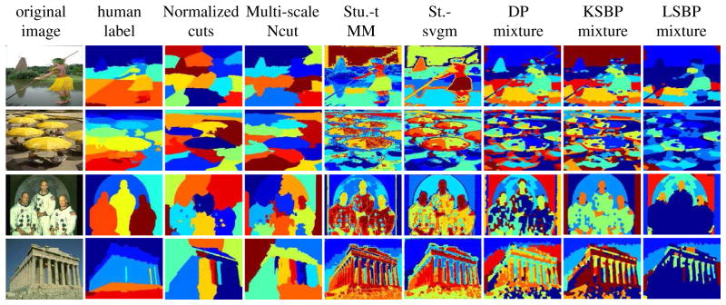
Figure 13 shows typical segmentation results for the different algorithms. Given a segment count number, both the normalized cuts and the multi-scale Ncut produced very smooth segmentations, while certain textured regions might be split into several pieces. The Student-t distribution mixture model (Stu.-t MM) yields a relatively robust segmentation, but it is sensitive to the texture appearance. Compared with Stu.-t MM, the spatially varying mixtures (St.-svgm) favors a more contiguous segmentation for the texture region, preserving edges; this may make a good tradeoff between keeping coherence and capturing details, but the segmentation performance is degraded by redundant boundaries, such as those within the goose body. Compared with these state-of-art algorithms, the LSBP results appear to be very competitive. Among the Bayesian methods (DP, KSBP and LSBP), LSBP tends to yield better segmentation, characterized by homogeneous segmentation regions and sharp segment boundaries.

Figure 13.

Segmentation examples of different methods with an initialization of K = 10. From top to down, each row shows: the original image, the image ground truth, normalized cuts, multiscale Ncut, Student-t distributions mixture model (Stu.-t MM), spatially varying mixtures (St.-svgm), DP mixture, KSBP mixture, and the LSBP mixture model.

To quantify segmentation results, we also calculated the Rand Index (RI) (Unnikrishnan et al., 2007) and the Variation of Information (VoI) (Meila, 2003), using segmentation “truth” provided with the data. RI measures consistency between two segmentation labels via an overlapping fraction, and VoI roughly calculates the amount of randomness that exists in one segmentation that is not explained by the other. Accordingly, for the RI measure, larger values represent better performance, and for VoI smaller values are preferred. We calculated the average RI and VoI values of the thirty images for each category; the statistics for the two measures are depicted in Tables 1 and 2, considering all 240 images and various K.

Table 1.

Statistics on the averaged Rand Index (RI) over 240 images as a function of K (Microsoft Research Cambridge images).

K		2	4	6	8	10
Ncuts	mean	0.5552	0.6169	0.6269	0.6180	0.6093
	median	0.5259	0.6098	0.6376	0.6286	0.6235
	st. dev.	0.0953	0.1145	0.1317	0.1402	0.1461
Multi-scale Ncuts	mean	0.6102	0.6491	0.6387	0.6306	0.6228
	median	0.5903	0.6548	0.6515	0.6465	0.6396
	st. dev.	0.0979	0.1361	0.1462	0.1523	0.1584
Stu.-t MM	mean	0.6522	0.6663	0.6409	0.6244	0.6110
	median	0.6341	0.6858	0.6631	0.6429	0.6360
	st. dev.	0.1253	0.1248	0.1384	0.1455	0.1509
St.-svgm	mean	0.6881	0.6861	0.6596	0.6393	0.6280
	median	0.6781	0.7026	0.6825	0.6575	0.6516
	st. dev.	0.1249	0.1262	0.1427	0.1532	0.1599
DP	mean	0.6335	0.6527	0.6389	0.6270	0.6187
	median	0.6067	0.6669	0.6431	0.6321	0.6232
	st. dev.	0.1272	0.1283	0.1384	0.1464	0.1507
KSBP	mean	0.6306	0.6530	0.6396	0.6290	0.6229
	median	0.5963	0.6693	0.6448	0.6371	0.6272
	st. dev.	0.1237	0.1303	0.1397	0.1464	0.1523
LSBP	mean	0.6516	0.6791	0.6804	0.6704	0.6777
	median	0.6384	0.6921	0.6900	0.6835	0.6885
	st. dev.	0.1310	0.1202	0.1263	0.1294	0.1319

Table 2.

Statistics on the Variation of Information (VoI) over 240 images as a function of K (Microsoft Research Cambridge images).

K		2	4	6	8	10
Ncuts	mean	1.7911	2.2034	2.4344	2.6885	2.8828
	median	1.8201	2.1990	2.4392	2.7134	2.8956
	st. dev.	0.4402	0.4213	0.4003	0.3673	0.3615
Multi-scale Ncuts	mean	1.7017	2.0538	2.3535	2.5548	2.7397
	median	1.7322	2.0238	2.3746	2.5912	2.7471
	st. dev.	0.4253	0.4276	0.4030	0.4056	0.4215
Stu.-t MM	mean	1.4903	2.0078	2.4258	2.7421	3.0085
	median	1.5312	2.0283	2.4653	2.7495	3.0341
	st. dev.	0.5161	0.4544	0.4120	0.3941	0.3798
St.-svgm	mean	1.4031	1.8957	2.2667	2.5764	2.7999
	median	1.4000	1.8957	2.2673	2.5919	2.8123
	st. dev.	0.5094	0.4176	0.4113	0.3956	0.4001
DP	mean	1.4810	1.9522	2.2961	2.5808	2.7740
	median	1.5145	1.9522	2.3541	2.6321	2.8432
	st. dev.	0.4952	0.3923	0.4186	0.4164	0.4573
KSBP	mean	1.4806	1.9383	2.3063	2.5888	2.7873
	median	1.4980	1.9811	2.3403	2.6304	2.8338
	st. dev.	0.4811	0.3919	0.4150	0.4128	0.4457
LSBP	mean	1.4484	1.8142	1.9811	2.1050	2.0861
	median	1.4631	1.8288	1.9825	2.1528	2.1178
	st. dev.	0.4835	0.4478	0.4979	0.5101	0.5254

Compared with other state-of-the-art methods, the LSBP yields relatively larger mean and median values for average RI, and relatively small average VoI, for most K. For K = 2 and 4 the spatially varying mixtures (St.-svgm) shows the largest RI values, while it does not yield similar effectiveness as K increases. In contrast, the LSBP yields a relatively stable RI and VoI from K = 4 to 10. This property is more easily observed in Figure 14, which shows the averaged RI and VoI evaluated as a function of K, for categories “houses” and “cows”. The Stu.-t MM, St.-svgm, DP and KSBP have similar performances for most K; LSBP generates a competitive result with a smaller K, and also yields robust performance with a large K.

Figure 14.

Average Rand Index (RI) and Variation of Information (VoI) as functions of K with image categories. (a) RI for “houses”, (b) RI for “cows”, (c) VoI for “houses”, (d) VoI for “cows”.

We also considered the Berkeley 300 data set.⁴ These images have size 481×321 pixels, and we also over-segmented each image into 1000 superpixels. Both the RI and VoI measures are calculated on average, with the multiple labels (human labeled) provided with the data. Each individual image typically has roughly ten segments within the ground truth. We calculated the evaluation measures for K = 5, 10 and 15. Table 3 presents results, demonstrating that all methods produced competitive results for both the RI and VoI measures. By a visual evaluation of the segmentation results (see Figure 15), multi-scale Ncut is not as good as the other methods when the segments are of irregular shape and unequal size.

Table 3.

Different segmentation methods compared on Berkeley 300 images data set.

	Normalized cuts	Multiscale Ncut	Stu.-t MM	St.-svgm	DP mixture	KSBP mixture	LSBP mixture
RI	0.7220	0.7404	0.7093	0.7188	0.7228	0.7237	0.7241
VoI	2.7857	2.5541	3.7772	3.5682	2.8573	2.7027	2.6591

Figure 15.

Segmentation examples of different methods with K = 10, for Berkeley image data set. From left to right, each column shows: the original image, the image ground truth, normalized cuts, multiscale Ncut, the Student-t distribution mixture model (Stu.-t MM), spatially varying mixtures (St.-svgm), DP mixture, KSBP mixture, and the LSBP mixture model.

The purpose of this section was to demonstrate that LSBP yields competitive segmentation performance, compared with many state-of-the-art algorithms. It should be emphasized that there is no perfect way of quantifying segmentation performance, especially since the underlying “truth” is itself subjective. An important advantage of the Bayesian methods (DP, KSBP and LSBP) is that they may be readily extended to joint segmentation of multiple images, considered in the next section.

5.4 Joint Image Segmentation with H-LSBP

In this section we consider H-LSBP for joint segmentation of multiple images. Experiments are performed on the Microsoft data, with another two unlabeled categories: “cloud” and “office”. Each category is composed of 30 images, and therefore there are 300 images in total, analyzed simultaneously. The same feature and image processing techniques are employed as above.

The H-LSBP automatically generates a set of indicator variables z_mn for each superpixel. The probability that the nth superpixel within image m is associated with the kth hidden indicator variable t_mk, is represented as p_k(s_mn) = σ(g_k(s_mn)) Π_l<k(1 − σ(g_l(s_mn))). By integrating out the distribution for each hidden indicator variable t_mk drawn from the global set of atoms ${\mathit{\theta }}_k^{\ast }$, we approximate the membership for each superpixel by assigning it to the cluster with largest probability. This “hard” segmentation decision is employed to provide labels for each data point (the Bayesian analysis yields a “soft” segmentation in terms of a full posterior distribution), as employed above when considering one image at a time.

Our goal is to segment all the images simultaneously, sharing model parameters (atoms) across all images. The results of this analysis are used to infer the inter-relationship between different images, of interest for image sorting and search. We set truncation levels L = 40 and K = 10 (similar results were found for larger truncations, and these parameters have not been optimized). As demonstrated below, the model automatically infers the total number of principal atoms shared across all images, and the number of atoms that dominate the segmentation of each individual image. The learning of these principal atoms, across the multiple images, is an important aspect of the model, so that the associated mixture weights with these atoms for each image can be regarded as a measurable quantity of inter-relationship between images (Blei et al., 2003; An et al., 2008). Specifically, similar images should have similar distributions over the model atoms. With the same inter-relationship measure generated from the HDP (Teh et al., 2005), H-KSBP (An et al., 2008) and the proposed H-LSBP, we may compare model utility as an image sorting or organizing engine.

To depict how the atoms are shared across multiple images with H-LSBP, we display an atom-usage count matrix in Figure 16, in which the size of each square size is proportional to the relative counts of that atom in a given image. Similar atom usage was revealed for HDP and H-KSBP (omitted for brevity), but the H-LSBP generally was more parsimonious in its use of atoms. This is attributed to the fact that the spatial continuity constraint within LSBP encourages a parsimonious representation (a relatively small number of contiguous clusters).

Figure 16.

Atom usage-count matrix for H-LSBP.

Each inferred image atom is in principle associated with one class of features within the images. To get a feel for how the model operates, we examine the types of image segments associated with representative atoms. Specifically, in Figure 17 we consider how eight representative atoms are distributed within example images. In this figure we show the original image, and also the same image with all portions not associated with a given atom blacked out. From Figure 17 we observe that atom 1 is principally associated with trees, atom 2 is associated with grass, atom 4 principally models offices, and atom 10 is mainly attributed to the surface of buildings. Figure 18 shows atom examples inferred from the H-KSBP and HDP, and the representative “cloud”, “grass”, “tree” and “street” atoms do not do as well in maintaining spatial contiguity. This property is especially important to locate certain objects or scenes. For example, for an image annotation task, it is usually expensive to acquire training data set by manually annotating image by image. Therefore, the H-LSBP might be used as an automatic annotation tool to save redundant manual work for the preprocessing the images with no words given.

Figure 17.

Demonstration of different atoms inferred by the H-LSBP model. The original images and associated connection to model-parameter atoms are shown on consecutive rows. All regions not associated with a respective atom are blacked out.

Figure 18.

Examples of different atoms inferred by the H-KSBP and HDP model: The first row is the original images; the second row is the atoms inferred by H-KSBP; the third row is the atoms inferred by HDP.

Based on the atoms inferred from Figure 16, we can jointly segment the 300 images with H-LSBP. Each atom represents a label, and the superpixels that shared the same atom are grouped together. Some representative segmentation examples are shown in Figure 19, in which each column shows one segmentation example with its “ground truth” (the second row), and the color bar encodes the labels/indexes of the results in the third row (the labels are re-ordered to be different from the atom index).

Figure 19.

Representative set of segmentation results of H-LSBP. The top row gives example images, the second row defines “truth” as given by the data set, and the third row represents the respective H-LSBP results.

Another interesting problem is to infer the inter-relationship between different images, and this may be achieved by quantifying the degree to which they share atoms (the sharing of the same set of atoms across all images plays an important role in inferring inter-image relationships). Since we know which atoms ${\{{\mathit{\theta }}_l^{\ast }\}}_{l=1}^L$ the superpixels within each image are drawn from, we may calculate the Kullback-Leibler (KL) divergence based on the histogram over atoms between each pair of images (a small value is added to the probability of each atom, to avoid numerical problems when computing the KL divergence, when the actual usage of particular atoms may be zero). The KL divergence between different categories, computed by averaging across all of the sub-class images, are shown in Figure 20. To make the figure easier to read, the KL divergence D_KL is re-scaled as exp(−D_KL). In Figure 20(a) results are shown based on the proposed H-LSBP, in (b) based upon an H-KSBP analysis, and in (c) based upon an HDP analysis. The H-LSBP, H-KSBP and HDP each yield good results, but Figure 20 indicates that the H-LSBP produces smaller cross-class similarity (additionally, the H-KSBP results are better than those of HDP).

Figure 20.

Similarity matrix associated with the ten image categories. (a) H-LSBP, (b) H-KSBP, (c) HDP

To demonstrate the utility of the proposed method in the context of an image sorting/search engine, we show image sorting examples in Figure 21. The left-most column is the original image, and columns 2–6 are the ordered five most similar images in the database, ordered according to the value of the KL divergence between the original image and the remaining 299 images. The five most similar images are shown in Figure 21, with generally good sorting performance manifested.

Figure 21.

Sample image sorting result, as generated by H-LSBP. The first left column shows the images inquired, followed by the five most similar images from the second to sixth column.

5.5 Computational Complexity

All the experiments in this paper were performed in Matlab on a Pentium PC with 1.73 GHz CPU and 4G RAM. For the audio-waveform example, 80 VB iterations for LSBP required 40 seconds. For the multi-task image segmentation, H-LSBP required nearly 7 hours of CPU to jointly segment 300 images, using 60 VB iterations (this CPU time may be cut in half if we only use 30 VB iterations, with minor degradation in performance). With both experiments, KSBP/H-KSBP typically required comparable CPU time, while DP/HDP required less than half the CPU time.

6. Conclusions

The logistic stick-breaking process (LSBP) is proposed for clustering spatially- or temporally-dependent data, imposing the belief that proximate data are more likely to be clustered together. The sticks in the LSBP are realized via multiple kernel-based logistic regression functions, with a shrinkage prior employed for favoring contiguous and spatially localized partitions. Competitive segmentation performance has been manifested in several examples. Relative to other related approaches, the proposed LSBP yields sharp segmentations, and is able to automatically infer an appropriate number of segments.

We also propose the hierarchical logistic stick-breaking process, H-LSBP, to segment multiple data sets simultaneously, with example results presented for images. The model parameters (atoms) are shared across all images, using a shared draw from a global DP prior. The total number of important atoms across all images, as well as the particular important atoms for a specific image, are inferred with an efficient variational Bayesian (VB) solution. Compared with the hierarchical Dirichlet process (HDP) and the hierarchical KSBP, the proposed method yields superior segmentation performance, based on studies with natural images. Further, we have investigated the ability of HDP, H-KSBP and H-LSBP to infer inter-relationship between different images, based on the underlying sharing of model atoms. The improved segmentation quality of the H-LSBP, relative to HDP and H-KSBP, also yields an improved ability to infer inter-image relationships.

Concerning future research, the results in Figure 17 indicate that the inferred atoms have connections to physical entities in images. This suggests that the model may be extended to the joint modeling of images and text (Barnard et al., 2003), with the text associated with aspects of the image. In addition, in the H-LSBP modeling of multiple images, the employed DP prior assumes that the order of the images is exchangeable (although LSBP imposes that spatial location within a particular image is not exchangeable). There are many applications (e.g., video) for which the multiple images may have a prescribed time index, that should be exploited. The results on the time-dependent audio data demonstrate how LSBP may also be employed to exploit temporal information.

The LSBP software is posted at www.ece.duke.edu\~lcarin\LSBP_code.rar

Appendix A. VB Update Equations for H-LSBP

For the model introduced in Section 3, we assume

$$q(\mathbf{\Phi })=q(\gamma )\prod _{l=1}^{L}q({\mathit{\theta }}_l)\prod _{l^{\prime }=1}^{L-1}q({\stackrel{\sim }{\beta }}_{l^{\prime }})\prod _{m=1}^M\left[\prod _{k^{\prime }=1}^{K}q(t_{{mk}^{\prime }})\prod _{k=1}^{K-1}[q({\mathbf{w}}_{mk})q({\mathbf{\lambda }}_{mk})\prod _{n=1}^{N_m}q(z_{\mathit{mnk}})]\right],$$

where q(θ_l) is the Dirichlet distribution, the same form as its prior p(θ_l|α₀). Then q(θ_l|α̃_l) is updated with a uniform prior specified for α₀ as follows:

$${\stackrel{\sim }{\alpha }}_{li}={\alpha }_{0i}+\sum _{m=1}^M\sum _{n=1}^{N_m}\sum _{k^{\prime }=1}^K<{\xi }_{mn,k^{\prime }}{>}_{q({\mathbf{z}}_{mn})}<t_{{mk}^{\prime },l}>y_{\mathit{mni}},$$

where α_0i = 1/I for i = 1, …, I, and I is the feature dimension; $<{\xi }_{mn,k^{\prime }}{>}_{q({\mathbf{z}}_{mn})}={\prod }_{k=1}^{k^{\prime }-1}(1-q(z_{mn}=k))·q(z_{mn}=k^{\prime })$ represents the approximated posterior probability that data D_mn is associated with the hidden “atom” t_mk′. For k′= K, ${\xi }_{mn,k^{\prime }}={\prod }_{k=1}^{k^{\prime }-1}(1-q(z_{mn}=k))$. Finally, < t_mk′,l > = q(t_mk′= l) represents the approximated posterior probability that t_mk′ takes the atom θ_l.

For updating q(β̃) and q(γ) given the prior p(γ) = Ga(γ|e₀, f₀), assume q(β̃_l) = Be(β̃_l|π_l1, π_l2) with l = 1, …, L, and q(γ) = Ga(γ|ẽ, f̃). Then the update equations are as follows:

$$\begin{array}{l}{\pi }_{l1}=1+{\sum }_{m=1}^M{\sum }_{k^{\prime }=1}^K<t_{{mk}^{\prime },l}>,\\ {\pi }_{l2}=\stackrel{\sim }{e}/\stackrel{\sim }{f}+{\sum }_{m=1}^M{\sum }_{k^{\prime }=1}^K{\sum }_{l^{\prime }=l+1}^L<t_{{mk}^{\prime },l^{\prime }}>,\\ \stackrel{\sim }{e}=e_0+L-1,\\ \stackrel{\sim }{f}=f_0-{\sum }_{l=1}^{L-1}\left[\psi ({\pi }_{l2})-\psi ({\pi }_{l1}+{\pi }_{l2})\right],\end{array}$$

in which ψ(·) is the Digamma function.

Given the approximate distribution of the other variables,

$$q(t_{{mk}^{\prime }}=l)\propto exp\left[<logp(t_{{mk}^{\prime }}\mid \mathit{\beta }){>}_{q(\mathit{\beta })}+<logp({\mathbf{y}}_m\mid t_{{mk}^{\prime }},{\mathbf{z}}_m,{\mathit{\theta }}_l){>}_{q({\mathbf{z}}_m),q({\mathit{\theta }}_l)}\right],$$

where < · >_q(·) represents the expectation of the associated variable’s distribution. One may readily derive that

$$q(t_{{mk}^{\prime }}=l)\propto exp[\sum _{l^{\prime }=1}^{l-1}[\psi ({\pi }_{l^{\prime }2})-\psi ({\pi }_{l^{\prime }1}+{\pi }_{l^{\prime }2})]+[\psi ({\pi }_{l1})-\psi ({\pi }_{l1}+{\pi }_{l2})]+\sum _{n=1}^{N_m}<{\xi }_{mn,k^{\prime }}{>}_{q({\mathbf{z}}_{mn})}<logp(y\mid {\mathit{\theta }}_l){>}_{q({\mathit{\theta }}_l)}],$$

where < log p(y|θ_l) >_q(θl) is the data likelihood, with expectation performed with respect to the distribution of atoms θ_l (which may be derived readily). Then q(t_mk′) = Mult(u_mk′1, …, u_mk′L), in which $u_{{mk}^{\prime }l}=\frac{q(t_{{mk}^{\prime }}=l)}{{\sum }_{l^{\prime }=1}^{L}q(t_{{mk}^{\prime }}=l^{\prime })}$.

Similarly, assume q(W_mk) = N(m̃_mk, Γ̃_mk) and q(z_mnk = 1) = ρ_mn,k = σ(h_mnk) for k = 1, …, K − 1, then

$$h_{\mathit{mnk}}=\sum _{k^{\prime }=k}^K{(-1)}^{{\nu }_{{kk}^{\prime }}}<{\xi }_{mn,k^{\prime }}^{-k}{>}_{q({\mathbf{z}}_{mn}^{-k})}\sum _{l^{\prime }=1}^{L}q(t_{{mk}^{\prime }}=l^{\prime })\left[<logp(y\mid {\mathit{\theta }}_l){>}_{q({\mathit{\theta }}_l)}\right]+{\stackrel{\sim }{\mathbf{m}}}_{mk}^T{\mathbf{x}}_{mn}^k,$$

where $<{\xi }_{mn,k^{\prime }}^{-k}{>}_{{\mathbf{z}}_{mn}^{-k}}={\prod }_{j=1,j\ne k}^{K-1}[{\rho }_{mn,j}{(-1)}^{{\nu }_{{jk}^{\prime }}}+{\nu }_{{jk}^{\prime }}]$ is the expectation associated the gating variables {z_mn1, …, z_mn(k−1), z_mn(k+1), …, z_mn(K−1)} except z_mnk, with the following definition for ν_kk′:

$${\nu }_{{kk}^{\prime }}=\{\begin{array}{ll}0\hfill & \text{if}{t}_{{mk}^{\prime }}\text{is}\text{in}\text{the}\text{left}\text{subtree}\text{of}{G}_{mk}(\text{see}\text{Fig}.5),\hfill \\ 1\hfill & \text{otherwise}.\hfill \end{array}$$

Assuming q(λ_mki) = Ga(ã_mki, b̃_mki), with i = 0, 1, …, N_c, the update equations for q(W_mk) are as follows:

$$\begin{array}{l}{\stackrel{\sim }{\mathbf{\Gamma }}}_{mk}={[2{\sum }_{n=1}^{N_m}f({\eta }_{\mathit{mnk}}){\mathbf{x}}_{mn}^k{{\mathbf{x}}_{mn}^k}^T+\text{diag}(\frac{{\stackrel{\sim }{\mathbf{a}}}_{mk}}{{\stackrel{\sim }{\mathbf{b}}}_{mk}})]}^{-1},\\ {\stackrel{\sim }{\mathbf{m}}}_{mk}={\stackrel{\sim }{\mathbf{\Gamma }}}_{mk}{\sum }_{n=1}^{N_m}\left[({\rho }_{mn,k}-1/2){\mathbf{x}}_{mn}^k\right],\end{array}$$

where the variational parameter

$${\eta }_{\mathit{mnk}}=\sqrt{{{\mathbf{x}}_{mn}^k}^T({\stackrel{\sim }{m}}_{mk}{\stackrel{\sim }{m}}_{mk}^T+{\stackrel{\sim }{\mathbf{\Gamma }}}_{mk}){\mathbf{x}}_{mn}^k},$$

and $f({\eta }_{\mathit{mnk}})=\frac{tanh({\eta }_{\mathit{mnk}}/2)}{4{\eta }_{\mathit{mnk}}}$ (Bishop and Svensen, 2003; Bishop and Tipping, 2000). The parameters ${\mathbf{x}}_{mn}^k$ are defined as ${\mathbf{x}}_{mn}^k=\{1,{\{K({\mathbf{s}}_{mn},{\widehat{\mathbf{s}}}_{mi};{\psi }_{mk})\}}_{i=1}^{N_c}\}$.

Given q(W_mk), the update equations for q(Λ_mk) are

$$\begin{array}{l}{\stackrel{\sim }{a}}_{\mathit{mki}}=a_0+1/2,\\ {\stackrel{\sim }{b}}_{\mathit{mki}}=\frac{1}{2}({\stackrel{\sim }{\mathbf{\Gamma }}}_{mk}(i,i)+{\stackrel{\sim }{m}}_{\mathit{mki}}^2)+b_0.\end{array}$$

References

- Ahonen T, Pietikäinen M. Image discription using joint distribution of filter bank responses. Pattern Recognition Letters. 2009;30:368–376. [Google Scholar]
- An Q, Wang C, Shterev I, Wang E, Carin L, Dunson DB. Hierarchical kernel Stick-breaking process for multi-task image analysis. Proceedings of the International Conference of Machine Learning; 2008. [Google Scholar]
- Antoniak CE. Mixtures of Dirichlet processes with applications to Bayesian nonparametric problems. Ann Statist. 1974;2(6):1152–1174. [Google Scholar]
- Banerjee S, Carlin BP, Gelfand AE. Hierarchical Modeling and Analysis for Spatial Data. 1. Chapman and Hall/CRC; 2003. [Google Scholar]
- Barnard K, Duygulu P, Forsyth D, Freitas ND, Blei DM, Jordan MI. Matching words and pictures. Journal of Machine Learning Research. 2003;3:1107–1135. [Google Scholar]
- Beal MJ. PhD thesis. The Gatsby Computational Neuroscience Unit, University College; London: 2003. Variational Algorithms for Approximate Bayesian Inference. [Google Scholar]
- Beal MJ, Ghahramani Z, Rasmussen CE. The infinite hidden Markov model. Proceedings of the Advances in Neural Information Processing Systems. 2002;14 [Google Scholar]
- Ben M, Betser M, Bimbot F, Gravier G. Speaker diarization using bottom-up clustering based on a parameter-derived distance between adapted GMMs. Proceedings of the International Conference on Spoken Language Processing; 2004. [Google Scholar]
- Bishop CM, Svensén M. Bayesian hierarchical mixture of experts. Proceedings of the Ninetheenth Conference of Uncertainty in Artificial Intelligence; 2003. [Google Scholar]
- Bishop CM, Tipping ME. Variational relevance vector machines. Proceedings of the sixth Conference of Uncertainty in Artificial Intelligence; 2000. [Google Scholar]
- Blackwell D, MacQueen JB. Ferguson distributions via Polya urn schemes. Ann Statist. 1973;1(2):353–355. [Google Scholar]
- Blei DM, Ng AY, Jordan MI, Lafferty J. Latent Dirichlet allocation. Journal of Machine Learning Research. 2003;3:993–1022. [Google Scholar]
- Cao L, Li F. Spatially coherent latent topic model for concurrent object segmentation and classification. Proceedings of ICCV; 2007. [Google Scholar]
- Caruana R. Multitask learning. Kluwer Academic Publishers; 1997. [Google Scholar]
- Chung Y, Dunson DB. Nonparametric Bayes conditional distribution modeling with variable selection. Journal of the American Statistical Association. 2009 doi: 10.1198/jasa.2009.tm08302. [DOI] [PMC free article] [PubMed] [Google Scholar]
- Cour T, Benezit F, Shi J. Spectral segmentation with multiscale graph decomposition. Proceedings of the IEEE International Conference on Computer Vision and Pattern Recognition; 2005. [Google Scholar]
- Duan JA, Guindani M, Gelfand AE. Generalized spatial Dirichlet process models. Biometrika. 2007;94(4):809–825. [Google Scholar]
- Dunson DB, Park J. Kernel Stick-breaking processes. Biometrika. 2007;95:307–323. doi: 10.1093/biomet/asn012. [DOI] [PMC free article] [PubMed] [Google Scholar]
- Escobar MD, West M. Bayesian density estimation and inference using mixtures. Journal of the American Statistical Association. 1995;90(430):577–588. [Google Scholar]
- Felzenszwalb PF, Huttenlocher DP. Efficient graph-based image segmentation. International Journal of Computer Vision. 2004;59:167–181. [Google Scholar]
- Fox EB, Sudderth EB, Jordan MI, Willsky AS. The sticky HDP-HMM for systems with state persistence. Proceedings of the International Conference on Machine Learning; 2008. [Google Scholar]
- Ganchev T, Fakotakis N, Kokkinakis G. Comparative evaluation of various MFCC implementations on the speaker verification task. Proceedings of the International Conference on Speech and Computer; 2005. [Google Scholar]
- Gersho A, Gray RM. Vector Quantization and Signal Compression. Springer; 1991. [Google Scholar]
- Gilks WR, Richardson S, Spiegelhalter D. Markov Chain Monte Carlo in Practice. 1. Chapman and Hall/CRC; 1998. [Google Scholar]
- Gomes R, Welling M, Perona P. Memory bounded inference in topic models. Proceedings of the International Conference of Machine Learning; 2008. [Google Scholar]
- Ishwaran H, James LF. Gibbs sampling methods for Stick-breaking priors. Journal of the American Statistical Association. 2001;96(453):161–173. [Google Scholar]
- Ishwaran H, Rao JS. Spike and slab variable selection: Frequentist and Bayesian strategies. Annals of Statistics. 2005 [Google Scholar]
- Meilă M. Comparing clusterings by the variation of information. Proceedings of the Sixteenth Annual Conference ofn Computational Learning Theory; 2003. [Google Scholar]
- Mori G. Guiding model search using segmentation. Proceedings of the International Conference on Computer Vision; 2005. [Google Scholar]
- Nguyen X, Gelfand AE. Technical Report T R 08-37. Dept. of Statistical Science, Duke University; 2008. The Dirichlet labeling process for functional data analysis. [Google Scholar]
- Orbanz P, Buhmann JM. Nonparametric Bayesian image segmentation. International Journal of Computer Vision. 2008;77:25–45. [Google Scholar]
- Pantofaru C, Schmid C, Hebert M. ECCV. 2008. Object recognition by integrating multiple image segmentations. [Google Scholar]
- Park J, Dunson DB. Statistica Sinica. 2009. Bayesian generalized product partition model. [Google Scholar]
- Petrone S, Guindani M, Gelfand AE. Hybrid Dirichlet mixture models for functional data. Journal Royal Statistical Society, Ser B. 2009 [Google Scholar]
- Rasmussen CE. The infinite Gaussian mixture model. Proceedings of the Advances in Neural Information Processing Systems. 2000;12 [Google Scholar]
- Ren X, Malik J. Learning a classification model for segmentation. In. Proceedings of the International Conference on Computer Vision; 2003. [Google Scholar]
- Sethuraman J. A constructive definition of Dirichlet priors. Statistica Sinica. 1994;2:639–650. [Google Scholar]
- Sfikas G, Nikou C, Galatsanos NP. Robust image segmentation with mixtures of student’s t-distributions. Proceedings of the IEEE International conference on Image Processing; 2007. [Google Scholar]
- Sfikas G, Nikou C, Galatsanos NP. Edge preserving spatially varying mixtures for image segmentaiton. Proceedings of the International conference on Computer Vision and Pattern recognition; 2008. [DOI] [PubMed] [Google Scholar]
- Shi J, Malik J. Normalized cuts and image segmentation. IEEE Transactions on Pattern Analysis and Machine Intelligence. 2000;22:888–905. [Google Scholar]
- Sudderth EB, Jordan MI. Shared segmentation of natural scenes using dependent Pitman-Yor processes. Proceedings of the Neural Information Processing Systems. 2008 [Google Scholar]
- Teh YW, Jordan MI, Beal MJ, Blei DM. Hierarchical Dirichlet processes. Journal of the American Statistical Association. 2005;101:1566–1582. [Google Scholar]
- Tipping ME. Sparse Bayesian learning and the relevance vector machine. Journal of Machine Learning Research. 2001;1:211–244. [Google Scholar]
- Tranter S, Reynolds D. An overview of automatic speaker diarisation systems. IEEE Trans on Audio, Speech, and Language Processing. 2006;14:1557–1565. [Google Scholar]
- Unnikrishnan R, Pantofaru C, Hebert M. Toward objective evaluation of image segmentation algorithms. IEEE Trans on Pattern Analysis and Machine Intelligence. 2007;29(6):929–944. doi: 10.1109/TPAMI.2007.1046. [DOI] [PubMed] [Google Scholar]
- Varma M, Zisserman A. Classifying images of materials: Achieving viewpoint and illumination independence. Proceedings of the 7th European Conference on Computer Vision (ECCV); 2002. [Google Scholar]
- Wang X, Grimson E. Spatial latent Dirichlet allocation. Proceedings of the Neural Information Processing Systems. 2007 [Google Scholar]
- Wei GCG, Tanner MA. A Monte Carlo implementation of the EM algorithm and the poor mans data augmentation algorithms. Journal of the American Statistical Association. 1990;85(411):699–704. [Google Scholar]
- Weijer JVD, Schmid C. Coloring local feature extraction. Proceedings of the 9th European Conference on Computer Vision; 2006. [Google Scholar]
- Winn J, Bishop CM. Variational message passing. J Machine Learning Research. 2005;6:661–694. [Google Scholar]
- Zabih R, Kolmogorov V. Spatially coherent clustering using Graph Cuts. Proceedings of CVPR’04; 2004. [Google Scholar]