Improving the accuracy of the structure prediction of the third hypervariable loop of the heavy chains of antibodies

Abstract

Motivation: Antibodies are able to recognize a wide range of antigens through their complementary determining regions formed by six hypervariable loops. Predicting the 3D structure of these loops is essential for the analysis and reengineering of novel antibodies with enhanced affinity and specificity. The canonical structure model allows high accuracy prediction for five of the loops. The third loop of the heavy chain, H3, is the hardest to predict because of its diversity in structure, length and sequence composition.

Results: We describe a method, based on the Random Forest automatic learning technique, to select structural templates for H3 loops among a dataset of candidates. These can be used to predict the structure of the loop with a higher accuracy than that achieved by any of the presently available methods. The method also has the advantage of being extremely fast and returning a reliable estimate of the model quality.

Availability and implementation: The source code is freely available at http://www.biocomputing.it/H3Loopred/

Contact: anna.tramontano@uniroma1.it

Supplementary Information: Supplementary data are available at Bioinformatics online.

1 INTRODUCTION

Antibodies are a class of Y-shaped proteins produced by B-cells that the immune system uses to identify and neutralize foreign pathogens such as bacteria and viruses. They have the remarkable ability to recognize virtually any foreign targets (the antigens) and bind to these with extraordinary affinity and specificity (Mian et al., 1991; Sliwkowski and Mellman, 2013). These characteristics make antibodies an ideal tool for the prevention and treatment of diseases such as cancer, infectious and cardiovascular diseases, arthritis, inflammation, immune disorders as well as for biotechnological applications (Mian et al., 1991; Sliwkowski and Mellman, 2013). Knowing the structure of antibodies is clearly instrumental for gaining insights into the biological phenomena of the antibody–antigen recognition as well as to interpret clinical data and rationally redesign the molecule for medical and biotechnological purposes (Ghiotto et al., 2011; Zibellini et al., 2010).

Antibodies are composed of two identical heavy and light chain pairs. The antigen binding site, present on the upper tips of the Y shape, is formed by six hypervariable (HV) loops also referred to as the complementary determining regions (CDRs). Three of the loops belong to the variable domain of the light chain, (L1, L2 and L3) and three to the variable domain of the heavy chain (H1, H2 and H3). The variability in these CDR loops in terms of loop length and amino acid compositions is the main reason of the antibody capability to bind many different antigens. The framework regions of antibodies are fairly well conserved, while the structural variations occur mostly in the CDR loops.

We and others have developed effective methods to predict the structure of antibodies (Choi and Deane, 2010, 2011; Sircar et al., 2009; Sivasubramanian et al., 2009). The strategy consists of modeling the framework by homology while the prediction of five of the six loops is based on the canonical structure (CS) model that states that these loops (the light chains loops and the H1 and H2 loops of the heavy chain) can only assume a limited number of conformations and that these are determined by the presence of key residues in specific positions in the sequence of the antibody (Chothia and Lesk, 1987; Tramontano et al., 1990). According to a recent blind assessment of the prediction accuracy of antibody modeling (Almagro et al., 2011), a good prediction can be obtained for non-H3 loops with an average root-mean square deviation (RMSD) of their Cα atoms close to 1 Å.

Only a partial CS model exists for the H3 loop, which allows the prediction of the structure of its four N-terminal and six C-terminal residues closer to the framework (Kuroda et al., 2008; Morea et al., 1998; Shirai et al., 1996). Accordingly, the prediction accuracy for H3 loops is not equally satisfactory as for the other loops, an important drawback because the H3 loop is central in the binding site and therefore often essential in determining the antibody–antigen interactions. In the above mentioned assessment (Almagro et al., 2011), none of the tested methods was able to provide sufficiently good predictions for H3; the average RMSD for the best methods was ∼3 Å. The high variability in length, structure and sequence of this loop is usually invoked as the main reason behind the difficulty of predicting its structure.

There have been several attempts to develop methods for predicting the structure of H3 loops, both template-based (Choi and Deane, 2011; Mandal et al., 1996; Marcatili et al., 2008) and template-free methods that try to predict the structure using ab initio conformation searches followed by ranking based on energy estimates and clash avoidance (Bruccoleri and Karplus, 1987; Sivasubramanian et al., 2009).

One of the most used approaches for antibody structure prediction is Rosetta Antibody (RA; Sircar et al., 2009; Sivasubramanian et al., 2009), which combines template selections with ab initio CDR H3 loop modeling (using loop fragments) and simultaneous optimization of the CDR loop conformations and Variable Light (VL)-Variable Heavy (VH) orientations. Another interesting approach is FREAD (Choi and Deane, 2010, 2011), which attempts to predict antibody loops using local similarities (local sequence and geometric matches). FREAD uses environment-specific substitution scores (Choi and Deane, 2010; Kelm et al., 2010; Lee and Blundell, 2009) to identify the best fragments for building the structure of the loops.

Each of the previous approaches has its own disadvantages and limitations, and this prompted us to develop the method described here. One of the main limitations of ab initio approaches (e.g. RA) is due to our incomplete understanding of the physicochemical principles governing protein structures, which leads to the employment of pseudo-energy approximate functions that are not always accurate in distinguishing correct predictions. In addition ab initio approaches tend to have high computational cost. On the other hand, the available homology-based methods such as FREAD-S (Choi and Deane, 2011) suffer from being essentially dependent on the H3 sequence alone that has proven to be insufficient to provide accurate models, especially for longer loops. The ConFREAD method (Choi and Deane, 2011) tried to overcome this limitation by including contact profile information; however, this only led to minor improvements obtained at the expense of a much lower coverage.

Given the central position of the H3 region in the antigen-binding site, there are several interactions with the other CDR loops, as well as with the framework, that could affect the conformation of H3 (Morea et al., 1998). In line with this hypothesis, we developed a method that takes advantage of sequence similarity and structural related features [e.g. CS (Chothia and Lesk, 1987; Tramontano et al., 1990) as well as a score reflecting the likelihood of the presence/absence of specific interactions between the H3 residues and the rest of the modeled antibody structure (Tung et al., 2007)].

We used a set of selected features to train a Random Forest (RF) machine learning algorithm to select the closest loop among a dataset of H3 loops present in immunoglobulins of known structure. The best predicted template(s) are used to build the structure of H3 that are subsequently ranked according to their intramolecular interactions. We tested our model on the RA benchmark (Sivasubramanian et al., 2009) (we used 53 of the 54 structures in the benchmark excluding the PDB: 2AI0 case because in RA benchmark the H3 loop was uncorrectly reported as a six-residue loop) and our results are more accurate than those provided by RA, considered the best method available at present, on the same benchmark. We also tested our method on recently deposited structures of antibodies with equally satisfactory results. Last but not least the described method requires substantially less computing time with respect to the RA (on average 5 min).

2 METHODS

2.1 Datasets

We scanned the sequences of all proteins in the PDB database (October 15, 2012) using isotype-specific Hidden Markov Model (HMM) profiles (Chailyan et al., 2012; Lefranc et al., 2009) to retrieve the structures of 1294 antibodies. We removed antibody molecules with resolution worse than 3 Å using the PISCES web server (Wang and Dunbrack, 2003). The resulting 1161 antibodies were clustered based on the sequence of H3 loops using the cd-hit package (Li and Godzik, 2006) with a sequence identity threshold of 90%. One representative antibody from each cluster was selected (priority was given to antibodies that were found to be in complex with their antigen in the crystal structure, using a procedure previously developed by us (Olimpieri et al., 2013). When this was not possible we selected the antibody with the longest H3 loop). As a result, we were left with 401 representative non-redundant antibodies.

The alignment of H3 loops was done according to (Chailyan et al., 2012; Lefranc et al., 2003; Morea et al., 1998) where insertions were introduced in the middle of the region comprised between the conserved residues Cys92 and Gly104. Throughout the article we use the Kabat–Chothia numbering scheme (Morea et al., 1998).

2.2 RF model

We used the R (v.4.6) implementation of the RF (randomForest package) and the RF regression tool to predict the 3D distance between pairs of H3-loop. For this specific purpose, the input features of the RF model are the sequences of the antibody pairs along with other sequence-derived features described below. The task of the RF model is to use these features to infer the 3D distance between each pair of H3 loops. In other words, for each loop in the testing set, we use our trained RF model to predict the distances between the target loop and all other loops in the training dataset. The loop predicted as the most similar to the target is used as template to build the model of the target H3.

2.3 TM-score as a similarity measurement

For calculating the 3D distances between H3 loops, we used the ‘TM-score’ algorithm implemented by Zhang and coworkers (Zhang and Skolnick, 2004). The main advantage of the TM-score over the perhaps most commonly used RMSD is that the TM-score weights more shorter distances between pairs of superimposed atoms than longer ones and does not require the definition of any cutoff distance. Moreover, the TM-score takes into considerations the difference in length between loops; hence, it is more appropriate for comparing loops of different lengths. The TM-score between two H3 loops was calculated using the Biopython Bio.PDB module (Hamelryck and Manderick, 2003) by superposing the stems of the two loops (residue H90–H92 and residue H104–H106 of the heavy chain) and calculating the pairwise distance between aligned residues; such distances were then converted to a TM-score (Zhang and Skolnick, 2004).

To compare our results with data available in the literature for other methods, we also computed the backbone RMSD between the selected templates and the target loops. Throughout the article we used ‘TM-distance’ (1 − TM-score) to represent the 3D distances between pairs of H3 loops.

2.4 Canonical structure

According to Chothia and Lesk (Chothia and Lesk, 1987; Tramontano et al., 1990), five among the six HV loops (L1, L2, L3, H1 and H2) are shown to adopt only a limited set of backbone conformations (named CS) that can be predicted on the basis of the position and nature of specific amino acids in given positions of the antibody sequence. As mentioned above, only a partial CS model could be derived for the H3 loop (Al-Lazikani et al., 1997; Morea et al., 1998). We used the CS of the six HV loops as variables for the RF model. The CS information was obtained using the tool provided by the DIGIT database (Chailyan et al., 2012).

2.5 Germline families

It has been advocated that the specific selected VH and VL Germline genes are essential for the understanding of the biophysical properties of antibodies (Ewert et al., 2003). In addition, a recent paper by Chailyan and coworkers (Chailyan et al., 2011) showed that Germline families are important for the overall structure of the antibody binding sites. Therefore, we also included the source organism and the Germline families as variables in our RF model.

2.6 BLOcks substitution matrix

The BLOcks substitution matrix (BLOSUM) matrix (Henikoff and Henikoff, 1992) is a substitution matrix commonly used to score alignments between evolutionary divergent protein sequences based on the local alignments of protein sequences. We used the BLOSUM40 scores between each aligned amino acids in pairs of the H3 loops as well as the score over the whole loop as variables for the RF model.

2.7 Structure alphabet substitution matrix

Structure alphabet substitution matrix (SASM; Tung et al., 2007) is a BLOSUM-like matrix, built taking into account substitution preferences for 3D segments between homologous structures with low sequence identity.

We included the score of the SASM matrix over the whole H3 loops as variable for the RF model.

2.8 RF variables

In summary we initially considered all the variables listed above to train our RF model, namely the full sequence of the antibody, the CSs, the Germline Families, BLOSUM40-based similarity and SASM-based similarity. We also included as variables the length differences of the six CDR loops (L1, L2, L3, H1, H2 and H3) between each pair of antibodies (target and template) and the length of the matching and non-matching gaps.

2.9 Redundancy reduction

There are two main sources of redundancy in our initial training dataset: The first source is the likely redundancy in the several RF variables (932) because they could be correlated and not all of equal relevance for the prediction task. The second source of redundancy is due to the fact that our training data includes all possible pairs of antibodies from our dataset of antibodies of known structure. This is bound to include a substantial amount of redundant information. This redundancy might introduce biases in our training model and consequently affect its prediction accuracy.

To address the problem of redundancy in the variables of RF model, we used the Mean Decrease Gini values (MDG), to rank each variable according to its importance. Following (Olimpieri et al., 2013) we also computed the average MDG (avMDG) and removed all variables with MDG lower than avMDG.

The following example illustrates the redundancy connected to the use of all possible pairs of antibodies: If we know the TM-distance between antibodies BF and FC, adding the TM-distance between BC can be redundant because the latter is correlated to the TM-distance between BF and FC. Consequently, we first used the whole TM-distance matrix between all possible pairs of H3 loops to build an undirected graph and next removed edges until no triangle is present in the graph.

To do so, we first find a suboptimal min-cut in the graph (weighted so that the two graph partitions that generate the min-cut have almost similar size) by means of a simulated tempering algorithm. We then remove all edges that start and end with nodes on the same side of the cut and retain only edges involved in the cut. Such reduced graph is, by definition, bipartite and therefore, according to the Turán's theorem (Turan, 1941), is triangle-free. Our final training set contains 401 nodes and 45 582 edges.

2.10 Model building and measurement of accuracy

First, we aligned the H3 loop of the 401 antibodies according to (Chailyan et al., 2012; Lefranc et al., 2003; Morea et al., 1998), removed from our dataset any antibody that shares >95% H3 sequence identity to the RA 53 testing cases (Sivasubramanian et al., 2009) obtaining a final dataset including 356 antibodies.

We next computed the TM-distances between each antibody pair in the training dataset and removed the redundancy as described in the previous section. Finally, we assigned the features described above to each pair of antibodies in the dataset.

The aim of the training phase is for the RF model to learn the TM-distance between the H3 of each pair of antibodies. In the first phase we used the RF to perform feature selection by retaining only the features the MDG of which is greater than the avMDG. Finally, we trained our model only using the selected features. We used a 5-fold cross validation to evaluate the performance, hence we trained the method on 4/5 of the data and tested it on the remaining 1/5. This step was repeated five times by randomly splitting the data into training and testing sets.

The final model is trained using the set of selected features, and its performance is assessed based on its accuracy in predicting the 53 testing cases of RA as well as the structure of 50 H3 loops from antibodies the structure of which has been deposited in the PDB database (www.rcsb.org) (Rose et al., 2013) after October 15, 2012.

In summary, given a target loop, we align it with all the loops in the training set and compute the selected features. The RF then provides the predicted TM-distance between the target loop and each loop in the training data.

2.11 Antibody modeling

Framework regions and non-H3 CDR loops were modeled using Prediction of Immunoglobulin structure (PIGS) (Marcatili et al., 2008) with default parameters. The predicted structure of the loop is then obtained via MODELLER (Sali and Blundell, 1993) using the loop(s) predicted to have the closer TM-distance to the input loop as template(s). The measure of model accuracy is the local backbone RMSD, calculated by superimposing the stems of the loops (as described before) and then calculating the RMSD of the H3 loop main chain atoms between the model loop and the native conformation.

2.12 H3 contact profile

To assess whether the structural environment information can be used to further refine the prediction of H3, we analyzed the interactions of H3 with residues belonging to the VH and VL domains and used them to build an interaction profile.

The 3D interaction information extracted from the training dataset is converted into a 2D table (reference contact matrix, CM) having H3 residues in the columns and environment residues in the rows. Each cell is assigned a value of 1 or 0 according to whether the H3 residue in the column makes or does not make a contact with a residue in the row in any immunoglobulin in the training dataset. Contacts were identified using the Dimplot program (Wallace et al., 1995) with default parameters. We built two matrices considering (i) the interactions occurring between H3 and residues belonging to the VH, VL and framework domains (external contacts), and (ii) the interactions occurring within H3 residues (internal contacts). Given a predicted H3 loop, its contact profile is computed as the sum of the contribution of both internal and external contacts, and a score [contact matrix similarity score (CM score), Equation 1] is assigned according to the Sokal–Michener distance (Seung-Seok Choi, 2010) between the observed (pCM) and reference contact matrices (rCM):

$$\text{CM score}=\frac{a+d}{a+b+c+d}$$ (1)

Where CM[i,j] is the value of the i-th row and j-th column of a CM, a is the number of ‘positive matches’ (pCM[i, j] = rCM[i, j] = 1, indicating the presence of contact in both reference and predicted matrix cells), d the number of ‘negative matches’ (pCM[i,j] = rCM[i,j] = 0, indicating the absence of contact in both cells) and b and c are the number of mismatches (pCM[i,j] ≠ rCM[i,j], meaning the presence of contacts in the reference matrix that are absent in the predicted matrix cell, and vice versa). The higher the similarity between pCM and rCM matrices the higher the CM score. The modeled loops are ranked accordingly.

3 RESULTS

Figure 1 illustrates the workflow of the template-based modeling that we developed for the structure prediction of H3. A detailed description of each step is provided in the Methods section.

Fig. 1.

Workflow of the H3 modeling procedure

Given an input antibody sequence, the RF model provides a predicted TM-distance (Zhang and Skolnick, 2004) between the target H3 loop and each of the loops present in our dataset of H3 loops of known structure. The loop with the lowest predicted TM-distance to the target is used as template to build the model of the target H3. When the value of the predicted TM-distance is >0.5, a reranking of the top-scoring RF templates is performed based on an environment CM score described below. The other CDR loops and the framework are modeled using the CS model as implemented in PIGS (Marcatili et al., 2008) for the framework, heavy and light chain packing, while the full antibody model is then assembled by grafting the selected H3 model.

3.1 Model validation

Table 1 summarizes the results obtained in a 5-fold cross validation experiment. The values represent the mean, standard deviation and median of the backbone RMSD between the target and the selected best template loop, respectively.

Table 1.

Five-fold cross validation results and comparison with BLOSUM40

Loop length	Number of structures	BLOSUM40	RF
Very short (4–6 residues)	40	1.6	1.3
Short (7–9 residues)	117	3.0	1.7
Medium (10–11 residues)	114	3.2	2.0
Long (12–14 residues)	94	3.6	3.5
Very long (>17 residues)	24	5.8	4.3
Mean RMSD		3.3	2.7
Median RMSD		2.4	1.8

The values in columns 3 and 4 are the average backbone RMSD (in Å) between the target and the selected best template loop.

The results show that the RF model achieved better results than a naive BLOSUM40 approach (that selects the H3 loop with the highest sum of the BLOSUM40 score computed between the sequence of the target and template loops) in 64% of the cases. These enhancements are even more obvious for loops of short and medium length (defined as 7–9 and 10–11 residues, respectively). This is expected because most of the training cases fall in these length ranges.

These results suggest that RF model features are suitable to efficiently find reliable structural templates better than what can be done by just sequence similarity.

One of the advantages of RF model is that it provides the possibility of analyzing the features and ranking them according to their contributions to the final prediction by using MDG. The 20 most relevant features in the case at hand are reported in Supplementary Table S1. These include BLOSUM, SASM, Germline families and CSs of specific CDR loops, H3 length, count of matching gaps, non-matching gaps in the H3 alignment and some specific residues. Figure 2 shows the residues that are predicted to have the greatest influence on the H3 structure. Interestingly, all these residues are close in structure to the H3 loop. This suggests that the surrounding environment of H3 loop might actually have an effect on the final structure of the loop.

Fig. 2.

Residues that contribute most to the selection of the H3 template. The structure shown is PDB ID: 2B4C. The H3 loop is shown in gold, the residues with MDG values above the average are indicated by spheres

Prompted by this observation, we also derived a knowledge-based approach to use this information for a better ranking of the potential predicted structures of the loop.

3.2 Model performance

To test the performance of our method and to compare it with the best available one, we tested the model on a widely used benchmark (Sivasubramanian et al., 2009) (RA dataset), consisting of 53 antibodies. Table 2 shows the average accuracy obtained on this dataset for the different loop length ranges. It can be noticed that the accuracy, in terms of backbone RMSD between model and native H3 loop conformations, varies with the difficulty of the target loops. Expectedly, the method performance reflects the availability of training structures over the different loop length ranges (Detailed results are provided in Supplementary Table S2). In other words, the method is dependent on the size of the training datasets; hence, we should expect that the performance will improve as the number of available immunoglobulin structures increases.

Table 2.

Performance of the different methods on the RA benchmark

Loop length	Number of Structures	RF	CM10	CM50	RF-CM10	RF-CM50	RA
Very short	3	1.3	1.3	1.3	1.3	1.3	1.4
Short	22	1.8	1.6	1.6	1.6	1.6	2.2
Medium	14	2.0	2.2	2.2	1.9	1.8	2.9
Long	10	3.6	2.8	3.7	2.9	3.3	3.5
Very long	4	4.9	6.0	7.2	6.0	7.1	7.6
Mean RMSD		2.4	2.3	2.5	2.2	2.4	3.0
Median RMSD		1.9	1.8	2.0	1.9	1.9	2.7
SD RMSD		1.5	1.5	1.9	1.6	1.9	2.1

The values in the last six columns are the average backbone RMSD (in A) between modeled and native H3 loops.

In 53% of the RA testing cases, the RF model was able to select a good H3 template (backbone RMSD between modeled and native H3 loop lower than 2 Å). Looking at specific cases, we can notice that the RF model significantly outperforms RA (ΔRMSD >1 Å) in 16 cases, whereas the opposite is true in only four cases. In summary, the RF model achieved better results than Rosetta in 57% of the cases generally in all the loop length ranges.

Notably, the correlation between the observed TM-distance and that predicted by the RF model is high, reaching a coefficient of 0.92 (Figure 3). This high correlation motivated us to use the predicted score as an approximate estimate for the accuracy of the results. A statistical analysis performed by Zhang and coworkers (Xu and Zhang, 2010) demonstrated that similar structures often have a TM-distance <0.5. Testing this hypothesis on the RA benchmark, we found that the selected template according to the RF model is reliable enough (RMSD: 1.5 ± 0.7 Å) when the predicted TM-distance is <0.5 (65% of the RA testing benchmarks), while the performance degrades substantially (RMSD: 3.8 ± 1.7 Å) when the predicted TM-distance is >0.5.

Fig. 3.

Correlation between the predicted and observed TM-distance on RA Benchmark

On the other hand, we found that even when the predicted TM-distance is >0.5, a better template is usually present among the top 10–50 RF-ranked templates.

Consequently, we decided to implement a CM score to rank the predictions in cases when the predicted TM-distance for the template is >0.5 threshold. The CM score, described in detail below, is based on a statistical analysis of the contacts between specific residues of H3 loops and other antibody residues. A high CM score indicates a good match between the interactions observed in the model and those present in antibodies of known structure. The overall performance of the CM score in ranking the models regardless of their predicted TM-distance is reported in Table 2 (details on the full RA dataset are reported in Supplementary Table S2). Notably, the performance is independent from the number of top-scoring templates used. In particular, despite the overall RMSD distribution is on average shifted toward higher RMSD values when considering 50 versus 10 RF templates (3.2 ± 2.0 and 2.6 ± 1.6 Å, respectively; details in Supplementary Table S2), the CM-based model ranking is essentially the same in the two cases (RMSD 2.5 ± 1.9 Å and 2.3 ± 1.5 Å). This indicates that the CM score is sufficiently robust and also indicates that the H3 environment information can be effectively used to reliably rank large sets of conformations of the same loop. When the CM-based ranking is used to rank the RF templates in cases where the highest predicted TM-distance is >0.5 (19 cases in the RA benchmark) the model accuracy improves in 10 cases (Figure 4), leading to the selection of a significantly better model in 5 cases (PDB ID: 1BQL, 1IQD, 1FBI and 1HZH, 4.3, 3.8, 7.7, 5.0 and 3.7 Å RMSD to 2.1, 2.1, 3.7 and 2.4 Å RMSD, respectively). Remarkably, combining the RF method with the ranking obtained with the CM score outperforms RA for all the loop length ranges, on average (Table 2), producing models with improved accuracy in 62% of cases and significantly improved (ΔRMSD >1 Å) in 33%. What is more relevant in our view is that, although on average the improvement brought about by using the combined method over the CM score strategy alone is not particularly high, combining the two methods provides a significant advantage in some of the difficult cases of long H3 loops (for example in the cases of antibodies 2ADG, 1IGM and 1BJ1, see Supplementary Table S2). The final results are summarized in Figure 5 and 6 where we show the results of the combined RF-CM model in comparison with the RA results and the actual best model in the dataset. In this case we used the top-scoring template proposed by RF when the predicted TM-distance is <0.5, while in the other cases we select the template using the CM score to resort the first 50 models. As it can be appreciated, this leads to a rather satisfactory level of accuracy. Interestingly, the actual closest template is correctly identified in one-fourth of the cases, and in 13% of cases the combined RF-CM method was able to produce model in the sub-angstrom accuracy range (RMSD < 1 Å). Comparatively, RA achieved the same accuracy range in one case only.

Fig. 4.

Improvement obtained by applying the CM score to cases where the predicted TM-distance is >0.5. The values of the RMSD of the best template present in the dataset are also shown. The loop length is indicated in parentheses below the corresponding PDB code

Fig. 5.

Overall performance of the combined RF-CM50 model with respect to RA. The values of the RMSD of the best template present in the dataset are also shown

Fig. 6.

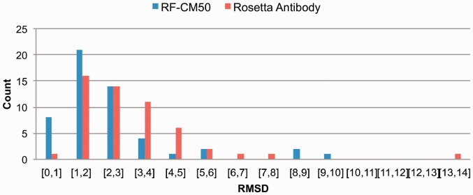
Overall performance of the combined RF-CM50 model with respect to RA

In a blind antibody modeling assessment experiment, Almagro et al. (2011) showed that, on average, all the tested methods preformed similarly, but also that in some CDR-H3 predictions the RA method was outperformed by other methods. We tested our approach on the same dataset used in the assessment and compared the results. In 75% of cases we were able to achieve similar or better accuracy compared with the best-performing method (Supplementary Table S3).

To assess the performance of the method in a more realistic setting, we downloaded the antibody structures that were added to PDB after October 15, 2012 (the date when we downloaded our training dataset). We selected those with resolution better than 3 Å and sharing <90% sequence identity among themselves and with H3 loops in the range of 3–20 residues. As a result, we obtained 50 target antibodies. Among these, we found a newly solved structure of the 4E10 antibody (PDB ID: 4LLV) that was already present in the training set (PDB ID: 2FX7) that we excluded from our analysis. Table 3 summarizes the results of this test (detailed results are in Supplementary Table S4). The combined RF-CM50 model was able to predict the loops with a mean RMSD 2.5 ± 1.5 Å. These results are rather satisfactory considering that the latter dataset is enriched of antibodies with long H3 loops. Moreover, in 14% of cases the selected model was in the sub-angstrom accuracy range.

Table 3.

Performance of the combined RF-CM model on 50 recently solved antibodies structures

Loop length	Number of structures	RF-CM10	RF-CM50
Very short	3	0.9	0.8
Short	11	1.3	1.7
Medium	18	2.4	2.1
Long	7	3.8	3.8
Very long	11	4.0	3.1
Mean RMSD		2.9	2.5
Median RMSD		2.6	2.2
SD RMSD		1.8	1.5

The values in columns 3 and 4 are the average backbone RMSD (in Å) between modeled and native H3 loops.

An in-depth analysis of the single cases revealed a substantial boosting of the combined RF-CM method with respect to each of them used separately (in 25% of the cases, the combined model improved the prediction accuracy of >1 Å with respect to each individual method). This indicates that the cutoff used is effectively able to discriminate good predictions from those that can be improved, sometimes drastically, by the CM score. In Figure 7 we illustrate three different cases that are paradigmatic of this behavior. Figure 7a shows an example (PDB ID: 4MSW) where the predicted low TM-distance (0.4) identifies a template close to the native conformation of the target loop, leading to a high-quality H3 model (RMSD = 0.3 Å). Another example is given by an 11-residue target loop, whose best RF template (PDB ID: 1TZI) has a higher predicted TM-distance (0.5). In this case our algorithm reranked the top 50 templates based on the CM-score and identified as top scored template the actual best one (PDB ID: 1YY9). This led to a significant improvement on the final model (from 3.1 to 0.4 Å, Figure 7b). In the last example, Figure 7c (PDB ID: 4LKC) the CM-based reranking allowed the selection of the best template available (PDB ID: 3GHE) for a 20 residues H3 loop with a final model RMSD of 2.7 Å.

Fig. 7.

Examples of accurate models obtained using the combined RF-CM50 method. a) Low TM-distance identifies a near native conformation; b) and c) CM-score reranking enhanced RF predictions for a medium and a long loop, respectively

4 CONCLUSIONS

In this study, we developed a new method for predicting the structure of H3 loops of immunoglobulins, a rather elusive and complex problem that is however essential for obtaining an accurate view of the antigen binding sites of this important class of molecules.

The method compares favorably with the most accurate available tool, i.e. RA with an average improvement of almost 1 Å in terms of average backbone RMSD. One important aspect of the method is that the average CPU time of our model is significantly shorter than Rosetta with an average CPU time (CPU speed: 2.5 GHz and RAM: 8 GB) of 5 min per antibody to be compared with hours and sometimes days for RA.

The prediction pipeline is currently being implemented in the context of PIGS (Marcatili et al., 2008), our widely used in house tool for immunoglobulin structure prediction.

We are currently investigating whether the ability of the RF method to select the meaningful variables and to properly learn from an extremely heterogeneous training environment, together with the redundancy reduction procedure we applied, can provide similarly satisfactory results in selecting the appropriate template for loops of proteins other than immunoglobulins.

REFERENCES

- Al-Lazikani B, et al. Standard conformations for the canonical structures of immunoglobulins. J. Mol. Biol. 1997;273:927–948. doi: 10.1006/jmbi.1997.1354. [DOI] [PubMed] [Google Scholar]
- Almagro JC, et al. Antibody modeling assessment. Proteins. 2011;79:3050–3066. doi: 10.1002/prot.23130. [DOI] [PubMed] [Google Scholar]
- Bruccoleri RE, Karplus M. Prediction of the folding of short polypeptide segments by uniform conformational sampling. Biopolymers. 1987;26:137–168. doi: 10.1002/bip.360260114. [DOI] [PubMed] [Google Scholar]
- Chailyan A, et al. The association of heavy and light chain variable domains in antibodies: implications for antigen specificity. FEBS J. 2011;278:2858–2866. doi: 10.1111/j.1742-4658.2011.08207.x. [DOI] [PMC free article] [PubMed] [Google Scholar]
- Chailyan A, et al. A database of immunoglobulins with integrated tools: DIGIT. Nucleic Acids Res. 2012;40:D1230–D1234. doi: 10.1093/nar/gkr806. [DOI] [PMC free article] [PubMed] [Google Scholar]
- Choi Y, Deane CM. FREAD revisited: accurate loop structure prediction using a database search algorithm. Proteins. 2010;78:1431–1440. doi: 10.1002/prot.22658. [DOI] [PubMed] [Google Scholar]
- Choi Y, Deane CM. Predicting antibody complementarity determining region structures without classification. Mol. Biosyst. 2011;7:3327–3334. doi: 10.1039/c1mb05223c. [DOI] [PubMed] [Google Scholar]
- Chothia C, Lesk AM. Canonical structures for the hypervariable regions of immunoglobulins. J. Mol. Biol. 1987;196:901–917. doi: 10.1016/0022-2836(87)90412-8. [DOI] [PubMed] [Google Scholar]
- Ewert S, et al. Biophysical properties of human antibody variable domains. J. Mol. Biol. 2003;325:531–553. doi: 10.1016/s0022-2836(02)01237-8. [DOI] [PubMed] [Google Scholar]
- Ghiotto F, et al. Mutation pattern of paired immunoglobulin heavy and light variable domains in chronic lymphocytic leukemia B cells. Mol. Med. 2011;17:1188–1195. doi: 10.2119/molmed.2011.00104. [DOI] [PMC free article] [PubMed] [Google Scholar]
- Hamelryck T, Manderick B. PDB file parser and structure class implemented in Python. Bioinformatics. 2003;19:2308–2310. doi: 10.1093/bioinformatics/btg299. [DOI] [PubMed] [Google Scholar]
- Henikoff S, Henikoff JG. Amino acid substitution matrices from protein blocks. Proc. Natl Acad. Sci. USA. 1992;89:10915–10919. doi: 10.1073/pnas.89.22.10915. [DOI] [PMC free article] [PubMed] [Google Scholar]
- Kelm S, et al. MEDELLER: homology-based coordinate generation for membrane proteins. Bioinformatics. 2010;26:2833–2840. doi: 10.1093/bioinformatics/btq554. [DOI] [PMC free article] [PubMed] [Google Scholar]
- Kuroda D, et al. Structural classification of CDR-H3 revisited: a lesson in antibody modeling. Proteins. 2008;73:608–620. doi: 10.1002/prot.22087. [DOI] [PubMed] [Google Scholar]
- Lee S, Blundell TL. Ulla: a program for calculating environment-specific amino acid substitution tables. Bioinformatics. 2009;25:1976–1977. doi: 10.1093/bioinformatics/btp300. [DOI] [PMC free article] [PubMed] [Google Scholar]
- Lefranc MP, et al. IMGT unique numbering for immunoglobulin and T cell receptor variable domains and Ig superfamily V-like domains. Dev. Comp. Immunol. 2003;27:55–77. doi: 10.1016/s0145-305x(02)00039-3. [DOI] [PubMed] [Google Scholar]
- Lefranc MP, et al. IMGT, the international ImMunoGeneTics information system. Nucleic Acids Res. 2009;37:D1006–D1012. doi: 10.1093/nar/gkn838. [DOI] [PMC free article] [PubMed] [Google Scholar]
- Li W, Godzik A. Cd-hit: a fast program for clustering and comparing large sets of protein or nucleotide sequences. Bioinformatics. 2006;22:1658–1659. doi: 10.1093/bioinformatics/btl158. [DOI] [PubMed] [Google Scholar]
- Mandal C, et al. ABGEN: a knowledge-based automated approach for antibody structure modeling. Nat. Biotechnol. 1996;14:323–328. doi: 10.1038/nbt0396-323. [DOI] [PubMed] [Google Scholar]
- Marcatili P, et al. PIGS: automatic prediction of antibody structures. Bioinformatics. 2008;24:1953–1954. doi: 10.1093/bioinformatics/btn341. [DOI] [PubMed] [Google Scholar]
- Mian IS, et al. Structure, function and properties of antibody binding sites. J. Mol. Biol. 1991;217:133–151. doi: 10.1016/0022-2836(91)90617-f. [DOI] [PubMed] [Google Scholar]
- Morea V, et al. Conformations of the third hypervariable region in the VH domain of immunoglobulins. J. Mol. Biol. 1998;275:269–294. doi: 10.1006/jmbi.1997.1442. [DOI] [PubMed] [Google Scholar]
- Olimpieri PP, et al. Prediction of site-specific interactions in antibody-antigen complexes: the proABC method and server. Bioinformatics. 2013;29:2285–2291. doi: 10.1093/bioinformatics/btt369. [DOI] [PMC free article] [PubMed] [Google Scholar]
- Rose PW, et al. The RCSB Protein Data Bank: new resources for research and education. Nucleic Acids Res. 2013;41:D475–D482. doi: 10.1093/nar/gks1200. [DOI] [PMC free article] [PubMed] [Google Scholar]
- Sali A, Blundell TL. Comparative protein modelling by satisfaction of spatial restraints. J. Mol. Biol. 1993;234:779–815. doi: 10.1006/jmbi.1993.1626. [DOI] [PubMed] [Google Scholar]
- Seung-Seok Choi SHC, Tappert CC. A Survey of Binary Similarity and Distance Measures. J. Syst. Cybern. Inf. 2010;8:6. [Google Scholar]
- Shirai H, et al. Structural classification of CDR-H3 in antibodies. FEBS Lett. 1996;399:1–8. doi: 10.1016/s0014-5793(96)01252-5. [DOI] [PubMed] [Google Scholar]
- Sircar A, et al. RosettaAntibody: antibody variable region homology modeling server. Nucleic Acids Res. 2009;37:W474–W479. doi: 10.1093/nar/gkp387. [DOI] [PMC free article] [PubMed] [Google Scholar]
- Sivasubramanian A, et al. Toward high-resolution homology modeling of antibody Fv regions and application to antibody-antigen docking. Proteins. 2009;74:497–514. doi: 10.1002/prot.22309. [DOI] [PMC free article] [PubMed] [Google Scholar]
- Sliwkowski MX, Mellman I. Antibody therapeutics in cancer. Science. 2013;341:1192–1198. doi: 10.1126/science.1241145. [DOI] [PubMed] [Google Scholar]
- Tramontano A, et al. Framework residue 71 is a major determinant of the position and conformation of the second hypervariable region in the VH domains of immunoglobulins. J. Mol. Biol. 1990;215:175–182. doi: 10.1016/S0022-2836(05)80102-0. [DOI] [PubMed] [Google Scholar]
- Tung CH, et al. Kappa-alpha plot derived structural alphabet and BLOSUM-like substitution matrix for rapid search of protein structure database. Genome Biol. 2007;8:R31. doi: 10.1186/gb-2007-8-3-r31. [DOI] [PMC free article] [PubMed] [Google Scholar]
- Turan P. On an extremal problem in graph theory. Matematikai es Fizikai Lapok. 1941;48:16. [Google Scholar]
- Wallace AC, et al. LIGPLOT: a program to generate schematic diagrams of protein-ligand interactions. Protein Eng. 1995;8:127–134. doi: 10.1093/protein/8.2.127. [DOI] [PubMed] [Google Scholar]
- Wang G, Dunbrack RL., Jr PISCES: a protein sequence culling server. Bioinformatics. 2003;19:1589–1591. doi: 10.1093/bioinformatics/btg224. [DOI] [PubMed] [Google Scholar]
- Xu J, Zhang Y. How significant is a protein structure similarity with TM-score = 0.5? Bioinformatics. 2010;26:889–895. doi: 10.1093/bioinformatics/btq066. [DOI] [PMC free article] [PubMed] [Google Scholar]
- Zhang Y, Skolnick J. Scoring function for automated assessment of protein structure template quality. Proteins. 2004;57:702–710. doi: 10.1002/prot.20264. [DOI] [PubMed] [Google Scholar]
- Zibellini S, et al. Stereotyped patterns of B-cell receptor in splenic marginal zone lymphoma. Haematologica. 2010;95:1792–1796. doi: 10.3324/haematol.2010.025437. [DOI] [PMC free article] [PubMed] [Google Scholar]
Associated Data
This section collects any data citations, data availability statements, or supplementary materials included in this article.