Random survival forests for competing risks

Abstract

We introduce a new approach to competing risks using random forests. Our method is fully non-parametric and can be used for selecting event-specific variables and for estimating the cumulative incidence function. We show that the method is highly effective for both prediction and variable selection in high-dimensional problems and in settings such as HIV/AIDS that involve many competing risks.

1. Introduction

Individuals subject to competing risks are observed from study entry to the occurrence of the event of interest, a competing event, or often, before the individual can experience one of the events, that person is right censored. Formally, let be the event time for the th subject, , and let be the event type, , where . Let denote the censoring time for individual such that the actual time of event is unobserved and one only observes and the event indicator . When , the individual is said to be censored at ; otherwise if , the individual is said to have an event of type at time . The observed data are where is a -dimensional vector of covariates.

We are interested in predicting events and in the discovery of risk factors. For the latter, we shall distinguish between risk factors for the cause-specific hazard and risk factors for the cumulative incidence. The cause-specific hazard function for event given covariates is

Here, is the event-free survival probability function given . The cause-specific hazard function describes the instantaneous risk of event for subjects that currently are event-free. Factors found to change the instantaneous event risk are associated with the biological mechanism behind event . On the other hand, the probability that an event occurs in a specific time period, say , depends on the cause-specific hazards of the other events (Gray, 1988). The probability of an event is determined using the cumulative incidence function (CIF), defined as the probability of experiencing an event of type by time ; i.e. . The CIF and cause-specific hazard function are related according to

(1.1)

Informally speaking, event can only occur for those surviving other risks. A covariate that reduces the cause-specific hazard of a competing risk increases the event-free survival probability and thereby indirectly increases the cumulative incidence of event . Thus, covariates found to change the -year risk of event (i.e. the cumulative incidence) are those that change the cause-specific hazard function of event and those that change the cause-specific hazard functions of the competing risks.

When the aim is to assist decision-making and for patient counseling we are interested in -year predictions and in finding covariates that affect the cumulative incidence. On the other hand, to understand and discuss treatment options for the biological mechanism that drives the risk of a specific event, we focus on the cause-specific hazard function.

In this paper, we propose a new approach to competing risks that builds on the framework of random survival forests (RSF) (Ishwaran and others, 2008), an extension of Breiman's random forests (Breiman, 2001) to right-censored survival settings. Our novel approach benefits from the many useful properties of forests and has following the important features: (a) it directly estimates the CIF; (b) it provides accurate prediction performance; (c) it models non-linear effects and interactions; (d) it can be used for event-specific selection of risk factors; (e) it can be used effectively in high-dimensional settings; and (f) it is free of model assumptions.

Section 2 describes the main parameters which we estimate by using ensembles. Section 3 describes the competing risks forest algorithm, introduces terminal node estimators used for constructing ensembles, and describes splitting rules for growing competing risk trees suitable for either cause-specific hazard or CIF inference. The prediction error for the proposed ensemble estimators and variable selection are discussed in Sections 4 and 5. Section 6 studies the performance of our method using synthetic data. In Section A of supplementary material available at Biostatistics online (http://www.biostatistics.oxfordjournals.org), we consider performance over a collection of well-known data sets. Section 7 utilizes RSF to identify event-specific variables using the Johns Hopkins HIV Clinical Cohort, a large database involving over 6000 HIV patients.

2. Parameters of interest

2.1. Expected number of life years lost and cause- mortality

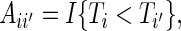
In addition to estimating the CIF, we propose a 1D summary of the cumulative incidence referred to as the expected number of life years lost due to cause (Andersen, 2012). In right-censored data, it is not feasible to get a reliable estimate of the expected lifetime. Therefore, for a fixed time point we consider the restricted mean lifetime conditional on : . The truncation time point is chosen such that the probability of being uncensored at is bounded away from zero: . In practice, we will typically set in accordance with the observed follow-up period (see Section 3). We extend the notation of Andersen (2012) to the case with covariates and note the relation , which holds for all values and all . The expected number of years lost before time is

Our summary value is , which the above shows equals the expected number of life years lost due to cause before time . We shall also call the cause- mortality.

2.2. Terminal node estimators

We describe non-parametric estimators of the event-free survival function, the cause-specific CIF, and mortality. The estimators are described here using the entire learning data set, but in implementation they are calculated within the terminal node of a RSF tree and then aggregated to form the ensemble (see Section 3.1).

Let denote the distinct and ordered event times from . Let be the number of type events at , and be the number of type events in . Define also , the total number of events occurring at time , , the total number of events occurring in , and , the number of individuals at risk (event-free and uncensored) just prior to . The Nelson–Aalen estimator for the cumulative event-specific hazard function is given by

where . The Kaplan–Meier estimator for the event-free survival function is given by

We use the Aalen–Johansen estimator (Aalen and Johansen, 1978) to estimate :

The cause- mortality is estimated by . We set to be the largest observed time .

3. Competing risk forests

A RSF (Ishwaran and others, 2008) is an collection of randomly grown survival trees. Each tree is grown using an independent bootstrap sample of the learning data using random feature selection at each node. RSF trees are generally grown very deeply with many terminal nodes (the ends of the tree). Trees in competing risk forests are grown similarly. What differs are the splitting rules used to grow the tree (Section 3.3) and the estimated values calculated within the terminal nodes used to define the ensemble (Section 3.1).

To grow a competing risk forest, we highlight two conceptually different approaches:

1. Separate competing risk trees are grown for each of the events in each bootstrap sample. The splitting rules used to grow the trees are event-specific.

2. A single competing risk tree is grown in each bootstrap sample. The splitting rules are either event-specific, or combine event-specific splitting rules across the events.

The second approach is more efficient (especially for high-dimensional problems and large data settings), sufficient for most tasks, and what we do in this article. In the next subsections, we describe how to calculate various ensembles useful for competing risks and provide details of competing risk trees. The forest algorithm is then summarized in Section 3.4.

3.1. Event-specific ensembles

Let denote the learning data. As stated earlier, a RSF tree is grown using an independent bootstrap sample of the learning data. Let be the number of times case occurs in bootstrap sample . To define the CIF for the th tree, take a case's covariate and drop it down the tree. Let denote the indices for cases from the learning data whose covariates share the terminal node with . Denoting node-specific event counts by and the number at risk by , we define 's CIF as

where is 's Kaplan–Meier estimate of event-free survival. The ensemble estimates of the CIF and the cause- mortality, respectively, equal

For reporting an internal error rate, we use out-of-bag (OOB) ensembles. By standard bootstrap theory, each bootstrap sample leaves out approximately 37% of the data. The OOB data are used to construct the OOB ensemble. Let be the index set of trees where ; i.e. records trees where case is OOB. The OOB ensemble estimates of the CIF and the cause- mortality are, respectively, given by

The OOB predicted value for a case does not use event time outcome information for that case, and, therefore, because it is a cross-validation based estimator, it can be used for estimation of the prediction error.

3.2. Event-free survival ensembles

An efficient method to analyze event-free survival probability is to simply use the tree-specific estimators already computed from the competing risks forests, which saves the computation time needed to grow a separate forest. Thus, we estimate the forest event-free survival using the ensemble .

3.3. Splitting rules

Here, we describe two splitting rules that can be used to grow competing risk trees. For notational convenience, we describe these rules for the root node using the entire learning data, but the idea extends obviously to any tree node and to bootstrap data.

As before, let denote the survival times and event indicators, and let be the distinct event times. Suppose that the proposed split for the root node is of the form and for a continuous predictor (this can be obviously generalized to categorical variables). Such a split forms two daughter nodes containing two new sets of competing risk data. To indicate these data, we use a subscript of and for the left and right daughter nodes, and denote by and the cause- specific hazard rates in the left and the right daughter nodes, respectively. Similarly, define and to be the CIF for the left and the right daughter nodes, respectively.

The number of individuals at risk at time in the left and right daughter nodes are, respectively, and , where , , and is the -predictor for individual . The number of individuals who are risk at time is . The number of type events at time for the left and right daughters is, respectively,

and is the total number of type events at . Define also to be the largest time on study in the parent node and the two daughters, respectively.

3.3.1. Generalized log-rank test

Our first splitting rule is the log-rank test. In the setting with competing risk, this is a test of the null hypothesis for all . The test is based on the weighted difference of the cause-specific Nelson–Aalen estimates in the two daughter nodes. Specifically, for a split at the value for variable , the splitting rule is

(3.1)

where the variance estimate is given by

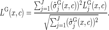
Time-dependent weights are used to make the test more sensitive to early or late differences between the cause-specific hazards. The choice corresponds to the standard log-rank test which has optimal power for detecting alternatives where the cause-specific hazards are proportional. The best split is found by maximizing over and .

3.3.2. Gray's test

The cause- specific log-rank splitting rule (3.1) is useful if the main purpose is to detect variables that affect the cause- specific hazard. It may not be optimal if the purpose is also prediction of cumulative event probabilities. In this case, better results may be obtained with splitting rules that select variables based on their direct effect on the cumulative incidence. For this reason, we model our second splitting rule after Gray's test (Gray, 1988), which tests the null hypothesis for all . For notational simplicity, consider analysis of event and assume ; that is, we pool all events not equal to event . Gray's statistic for testing the null is

where Here, the variance estimate is estimated based on the asymptotic normal representation under the null hypothesis; see bib11 for details.

In the special case where the censoring time is known for those cases that have an event before the end of follow-up, it is possible to obtain the score statistic of Gray's test by a simple modification of the log-rank test statistic. This is achieved by substituting in (3.1) for the modified risk set:

This motivates our modified splitting rule. The splitting rule based on the score statistic that uses the modified risk sets is denoted by and given by substituting for and for in (3.1). Note that if the censoring time is not known for those cases that have an event before the end of follow-up, the largest observed time is used, and the statistic is still a good (and computationally efficient) approximation of Gray's test statistic; see Fine and Gray (1999, Section 3.2).

3.3.3. Composite splitting rules

If the aim is to predict the CIF of all causes simultaneously, or if interest is in identifying variables that are important for any cause, it can be useful to combine the cause-specific splitting rules across the event types:

(3.2)

(3.3)

The best split is found by maximizing over and . Note that we have ignored the dependence in the test statistics in defining the variance. We do so because these types of calculations are not suitable for random forest trees. As these trees are grown deeply, tree nodes typically have few observations, which makes estimation of a covariance matrix problematic due to the limited data and will result in a poorly performing split-statistic. We should remark that a bias may occur with (3.3) if the censoring times remain unknown for cases that have an event before the end of the follow-up. However, our empirical results indicate that, for the purpose of building competing risk forests, the modified Gray splitting rule performs very well.

3.4. Competing risks forest algorithm

The steps required to construct a competing risks forest can be summarized as follows.

1. Draw bootstrap samples from the learning data.

2. Grow a competing risk tree for each bootstrap sample. At each node of the tree, randomly select candidate variables. The node is split using the candidate variable that maximizes a competing risk splitting rule.

3. Grow the tree to full size under the constraint that a terminal node should have no less than unique cases.

4. Calculate and for each tree, .

5. Take the average of each estimator over the trees to obtain its ensemble.

4. Prediction performance

4.1. Performance metrics

To assess prediction performance, we use the concordance index and the prediction error defined by the integrated Brier score (BS). The concordance index (C-index) is related to the area under the receiver operating characteristic curve and estimates the probability that, in a randomly selected pair of cases, the case that fails first had a worse predicted outcome. The BS is the squared difference between actual and predicted outcome.

Individuals are ranked by ensemble cause- mortality. We say that case has a higher risk of event than case if 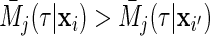. Wolbers and others (2013) described a time-truncated concordance index for competing risks, which in our setting is

Thus, the ensemble prediction of the cumulative incidence is concordant with the outcome if either the case with the higher cause- mortality has event before the other case has an event of cause or if the other case has a competing event. We also consider the time-dependent BS (Graf and others, 1999; Gerds and Schumacher, 2006) and its integral (IBS) to assess the performance of the ensemble CIF:

4.2. OOB estimate of prediction error

Denote for the right-censored observations in a validation data set of size . Based on these data, the prediction error can be estimated using inverse probability of censoring weights (IPCWs) (Gerds and Schumacher, 2006; Wolbers and others, 2013). This technique requires an estimate of the censoring distribution. Let denote the so-called reverse Kaplan–Meier estimate of the censoring distribution. We shall assume that the censoring times are independent of the covariates and the event times and the event type. Thus, provides an unbiased estimate of the probability of being uncensored at time . To estimate we define weights and 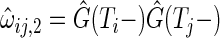. The OOB-IPCW estimate at the largest observation time is

where , and . Using weights (Binder and others, 2009), the OOB estimate of the integrated BS for event is given by

Note that extremely large weights may occur, but can be avoided by evaluating the IPCW statistics at an earlier time point .

5. Variable selection

5.1. Variable importance

RSF variable selection typically involves filtering variables on the basis of variable importance (VIMP). VIMP measures the increase (or decrease) in prediction error for the forest ensemble when a variable is randomly “noised-up” (Breiman, 2001). A large positive VIMP shows that the prediction accuracy of the forest is substantially degraded when a variable is noised-up; thus a large VIMP indicates a potentially predictive variable.

In Breiman's original definition, VIMP is calculated by noising up a variable by permuting its value randomly. A more effective noising-up method, and one used throughout this paper, is random node assignment (Ishwaran and others, 2008). In random node assignment, cases are dropped down a tree and randomly assigned to a daughter node whenever the parent node splits on the target variable. This is more effective than permutation since it leads to a random assignment regardless of the type of variable. For example, permuting a discrete variable with, say, two values may not lead to a sufficiently noised-up feature.

Both non-event-specific and event-specific VIMP can be readily calculated for competing risks. To compute event-specific VIMP, we estimate the prediction error as described in Section 4.2. Then we noise up the data by random node assignment, and recompute the prediction error. The difference in these two values gives the VIMP for each variable for each event .

5.2. Minimal depth

Minimal depth assesses the predictiveness of a variable by the depth of the first split of a variable relative to the root node of a tree (Ishwaran, Kogalur, Gorodeski and others, 2010). The smaller this value, the more predictive is the variable. There are unique advantages to using minimal depth in a competing risk setting. First, unlike VIMP, there is an easily derived minimal depth threshold that can be used for selecting variables. Secondly, minimal depth is non-event-specific, and therefore by fitting a single forest it can be used to identify all variables that affect long-term event probabilities. On the other hand, while non-event-specific analyses are useful, it may also be important to identify variables that are event-specific. In Section 6.2, we describe a simple way to combine minimal depth with event-specific VIMP.

6. Empirical results

6.1. Simulations

We used simulations based on Cox-exponential hazard models of two competing events () given a vector of covariates . In all simulations, we set . Six continuous predictors were drawn independently from a standard normal distribution and six binary predictors from a binomial distribution with success probability of 50%. We set

such that variables , , , have an effect on the hazard of event 1 only, variables , , , have an effect on the hazard of event 2 only, and variables , , , have an effect on both hazards. The effect size for the continuous variables was set to and for the discrete variables the effect size was set to 1.5. This was our “linear model”. The additive structure of the linear model was changed in our “quadratic model”. Here, the squared variables, , have an additional effect on the event-specific hazards where

Finally, we consider an “interaction model”. Additional interaction effects were added to the linear model of the form

We set the effect sizes of the interaction terms to

In all three simulation models, independent noise variables were drawn independently from a standard normal distribution and added to the simulated data sets. We set in our low-dimensional scenarios and in our high-dimensional scenarios. In all settings, independent right censoring was induced by drawing censoring times from an exponential distribution with rate . This yielded approximately 33% censored observations.

6.2. Forest models

The R-package randomForestSRC (Ishwaran and Kogalur, 2013) was used for computations. For each simulation experiment, 1000 trees were grown using the log-rank splitting rule (3.2) and the modified Gray's splitting rule (3.3). Terminal node size was set at (the default software setting). Randomized splitting was used. Within each parent node, for each of the randomly selected candidate variables, “nsplit” randomly selected split points were chosen (this is in contrast to non-random splitting where all possible split points for each of the candidate variables are considered). The tree node was split on that variable and random split point maximizing the absolute value of the split-statistic. We set nsplit . A small nsplit value is necessary in settings involving a mixture of discrete and continuous variables to avoid biasing splits toward continuous variables (Loh and Shih, 1997; Ishwaran, Kogalur, Gorodeski and others, 2010).

We fit RSF using log-rank splitting (3.2) for each event using weights and . We denote the resulting forests as and . Because we focus on performance over event 1 only (for ease of interpretation), we only report the results for . Additionally, three forests were fit using Gray's modified splitting rule (3.3): used ; used ; used . Only and are reported.

Variables were selected using minimal depth variable selection Ishwaran, Kogalur, Gorodeski and others (2010). Those variables whose event-specific VIMP was positive, and that met a minimal depth threshold (estimated from the forest), represented the final selected set of variables. As noted in Ishwaran, Kogalur and others (2010), the number of variables selected at each node, , referred to as “mtry”, should be set high when using minimal depth in high-dimensional applications. In our high-dimensional simulations (), we used . The default setting was used in low-dimensions (). See Ishwaran, Kogalur and others (2010) for further discussion on setting tuning parameters in high dimensions.

For comparison, we used four alternative methods. For the first, we used the proportional subhazard method of Fine and Gray (1999), abbreviated as FG and FG. Computations were implemented using the R-software package cmprsk (Gray, 2006). For the second method, we used cause-specific Cox regression (abbreviated as and ) for each of the competing events. Predictions of the CIF were obtained by combining the Cox models using (1.1). Computations were implemented using the R-software riskRegression (Gerds and others, 2012). For both approaches, we specified additive effects of the predictor variables and resorted to selecting variables by using -values. A cutoff of 5% was used. For the third method, we applied a stepwise selection algorithm (CRRstep) to the Fine-Gray regression models as proposed in Kuk and Varadhan (2013). We used backward elimination as implemented in the R-package crrstep with an Akaike information criterion selection criterion (Varadhan and Kuk, 2013). For the fourth method, we used Cox-likelihood based boosting (Binder and Schumacher, 2008), abbreviated as CoxBoost and CoxBoost. This uses boosting to fit proportional subhazards as in Fine and Gray (1999). Computations were implemented using the CoxBoost R-software package (Binder, 2009). The optimal number of boosting iterations was estimated using 10-fold cross-validation. A boosting penalty of 100 was used.

6.3. Simulation results

The simulations were repeated 1000 times independently and results were averaged over the runs. To estimate prediction performance (Table 1), in each simulation run we generated a training set with independent observations and a test set with independent observations. The C-index and the integrated BS were truncated at a sufficiently low quantile of the observed event time distribution. A lower benchmark for prediction performance was obtained in each simulation study by fitting a null model which ignores all covariates. An upper benchmark was obtained by fitting the data generating model to each training data set, i.e. the combination of two cause-specific Cox regression models that were given the correct linear predictor (including quadratic and interaction terms) and no noise variables.

Table 1.

Cox-exponential simulations replications)

	Low-dimensional simulations
	, ,
	Linear model		Quadratic model		Interaction model
NM	15.4 (0.7)	—	15.1 (0.6)	—	15.5 (0.6)	—
	10.1 (0.6)	82.1 (1.4)	9.5 (0.7)	79.4 (2.2)	10.8 (0.7)	80.3 (1.5)
	13.6 (0.7)	75.9 (2.3)	13.9 (0.7)	72.1 (2.6)	15.1 (0.6)	61.6 (2.5)
	13.2 (0.7)	76.5 (2.1)	13.6 (0.6)	72.0 (2.4)	15.0 (0.6)	61.3 (2.6)
	13.1 (0.6)	77.2 (2)	13.5 (0.6)	72.9 (2.3)	15.0 (0.6)	61.9 (2.5)
CoxBoost	11.4 (0.7)	79.6 (1.9)	13.9 (0.8)	65.7 (4)	15.4 (0.7)	55.9 (4.1)
FG	11.7 (0.9)	79.5 (1.8)	14.6 (1.0)	66.4 (2.7)	16.5 (0.9)	57.5 (2.5)
	10.9 (0.7)	80.1 (1.7)	14.4 (1.0)	66.6 (2.6)	16.5 (0.9)	57.6 (2.5)
CRRstep	13.6 (2.1)	62.7 (18.4)	14.8 (0.9)	55.4 (12.1)	15.7 (0.7)	49.7 (9.1)

	High-dimensional simulations
	, ,
	Linear model		Quadratic model		Interaction model
NM	15.4 (0.7)	—	15.1 (0.6)	—	15.5 (0.6)	—
DGM	10.1 (0.6)	82.0 (1.4)	9.8 (0.9)	79.3 (2.2)	10.8 (0.7)	80.3 (1.5)
	14.9 (0.7)	67.4 (2.9)	14.8 (0.7)	65.0 (3.6)	15.5 (0.7)	53.3 (2.5)
	14.9 (0.7)	65.8 (3.5)	14.6 (0.7)	64.5 (3.4)	15.6 (0.6)	52.2 (2.4)
	14.8 (0.7)	68.3 (3.1)	14.4 (0.6)	66.7 (3.2)	15.6 (0.6)	52.7 (2.5)
CoxBoost	13.5 (1.0)	72.0 (4)	14.8 (0.8)	58.4 (5.7)	15.7 (0.7)	51.5 (2.9)

Performance measures are average (standard deviation) of test set C-index and integrated BS . NM is the null model which assigns the same predicted CIF to each observation and is the data generating model fitted to the training set.

Based on Table 1, we draw the following conclusions:

1. In the low-dimensional linear simulations, Fine–Gray, Cox, and CoxBoost are better than RSF.

2. For the low-dimensional quadratic and interaction model, RSF outperforms the other methods.

3. RSF is better than CoxBoost in the high-dimensional quadratic and interaction model simulations, but CoxBoost is better in the linear model.

4. The event-specific RSF models and tended to be slightly better than the composite model in the low-dimensional simulations, but this trend was less pronounced in the high-dimensional simulations, and in some cases it was reversed (high-dimensional linear model).

5. We were not able to calculate Fine–Gray or Cox in the high-dimensional simulations. This is expected of unregularized methods which perform poorly in high-dimensional problems.

To assess VIMP, we calculated selection rates across the 1000 runs (Tables 2 and 3). True positive rates were summarized separately for each of the predictors . False positive rates were averaged across noise variables. Based on Tables 2 and 3, we draw the following conclusions:

1. The log-rank splitting forest performs best in identifying only those variables affecting the event 1 cause-specific hazard (i.e. and ). Recall that log-rank splitting is designed to test for differences in the cause-specific hazard: the results confirm the efficacy of the approach.

2. The Gray composite splitting forest is designed to discover all variables affecting the event 1 CIF, which are . We find it does a good job doing so. Furthermore, in nearly all simulations, it achieves the smallest false positive rate over the noise variables.

Table 2.

Variable selection frequencies from low-dimensional simulation study

													Noise
Linear model
	34.4	37	17.1	17.6	85.3	85.4	42.4	42.2	16.7	18	94.1	94.1	2.0
	90.3	91.2	22	19.7	39.5	42.4	94.1	94.5	17.5	18.8	39.1	39.2	7.5
	88.4	88.9	6.5	6	81.8	81.6	93.2	94.4	2	2.6	88.4	86.6	5.2
CoxBoost	99.9	99.7	78.2	75.8	91.4	91.6	99.9	100	82.5	80.5	95	94.4	37.6
	99.7	100	7.1	7.1	99.9	99.5	99.9	99.9	7	5.5	100	99.9	0
	99.6	99.6	9.5	8.2	99.4	99.6	99.9	99.8	8.9	8.5	99.8	99.6	8.9
FG	97.8	97.3	41	42	70	72.2	99.2	99.3	48.7	46.9	79.8	77.4	8.9
CRRstep	48.8	48.9	31.2	31.5	42.7	42.6	49	49.1	35.2	33.5	44.9	45.1	11.5
Quadratic model
	79.1	42.9	35.9	14.1	91.8	97.9	8.2	10	6.1	3.7	31.1	31.9	3.8
	99.9	84.1	23.3	18.9	59.2	42	31.1	32.9	7.4	7.5	10.6	9.6	7.6
	100	80.7	5.5	6.2	96.4	83.6	27.5	30.9	2.5	2.4	23.8	22.5	6.4
CoxBoost	92	83.5	60.9	46.3	57.9	70.1	68.3	66.4	37.5	38.6	46.2	43.4	28.7
	100	97.2	7.1	6.7	99.6	97.6	72.1	74.2	7.5	7.2	72.8	71.4	0
	92.9	66.7	10.5	9.3	76.6	69.9	45.3	46.3	8.2	9.6	41.1	37.8	8.4
FG	80.3	66.1	34.8	18.9	30.4	44.5	39.3	40.7	12.1	12.3	18.4	16.5	7.2
CRRstep	43.6	35.9	23.3	18	26.1	28.1	27.8	28.7	13.6	13	16.5	15.5	9.7
Interaction model
	28.3	27.2	18.1	18.5	65.2	59.5	20.5	27.7	8.9	11	66.5	57	14.2
	50.1	57.2	20.2	18.9	27.5	26.6	45.5	61.1	10.4	13.9	19.8	17.4	17.1
	48.1	57.4	17.4	16.6	43.3	44.6	46.2	62.1	5.8	5.2	45.4	42.3	17.7
CoxBoost	23.3	17	16.6	16.4	16.7	15	50.2	59.8	22.4	28.9	31.5	27.6	14.9
	99.1	96.9	7	6.4	97.4	97.1	56	45	6.1	6.1	54.1	50.3	0
	19	8.3	8.7	7.6	14.1	7.9	46.8	59.1	7.9	6.7	47.4	40.4	8.0
FG	15.2	7	8.5	6.5	7.2	6.7	40.2	54.5	12	14.4	22.5	19.5	6.5
CRRstep	15.8	5.7	6	5.8	5.8	5.9	19.8	22	9.1	5	7.4	6.2	5.7

Variables have an effect on the hazard of event only variables have an effect on the hazard of event only and variables have an effect on both hazards. Shown are the true positive rates separately for variables –. False positive rates over the noise variables are given in columns labeled “Noise”.

Table 3.

Variable selection frequencies from high-dimensional simulation study , ,

													Noise
Linear model
	15.3	15	7.7	7	54.8	53.9	21.4	23.3	9.5	9.9	83.4	81.5	1.6
	53.5	51.7	5.5	6.6	16.2	17	64	67.1	6.4	4.9	11.6	10	3.4
	44.5	44.8	1.4	1.4	35.7	35.3	56.6	59.8	0.3	0.1	48.2	44.6	1.4
CoxBoost	89.9	91.2	26.8	27.3	47.2	46.5	93.6	93.6	33.6	31.3	57.8	53.6	3.9
	99.9	99.8	8.4	6.3	99.8	99.7	100	100	6.2	4.7	99.8	100	0
Quadratic model
	60.8	22.2	24.5	11.9	82.7	95.4	4.8	4.5	3.6	4.1	16.2	18.4	1.5
	99.4	30.7	6	12.4	48.4	8.2	12.3	11	1.4	2.4	2	2.7	3.7
	99.1	31.1	3	5.8	93.5	40.4	13.4	12.7	0.6	1.2	8.6	9.5	4.5
CoxBoost	68.7	32.7	13.4	8	16.7	18.3	18.1	18.7	3.2	4.7	5.6	5.1	1.8
DGM	100	96.6	7.5	7.7	99.8	97.9	69.8	72.8	6.1	8.2	71.2	70.9	0
Interaction model
	3.8	4.4	4.5	3.5	10	9.8	7.7	13.4	6.6	7.3	38.1	33	2.6
	10.2	9.7	6.2	4.2	5.3	6.4	15.1	25.7	2.7	3.3	4.3	3.9	4.4
	10.8	12.3	7.3	4.4	10.5	11.6	15.8	25.8	1.6	1.2	17.7	15.9	5.4
CoxBoost	2.6	1.8	1.4	1.2	1.3	1.6	15.5	25.7	3.9	5.2	6	6.1	1.2
	97.9	97	6.8	7.7	98.5	97.3	56.8	46.8	8.5	7.7	54	47.9	0

Variables , , , have an effect on the hazard of event 1 only, variables , , , have an effect on the hazard of event 2 only, and variables , , , have an effect on both hazards. Shown are the true positive rates separately for variables –. False positive rates over the noise variables are given in columns labeled “Noise”.

7. Highly active antiretroviral therapy for HIV infection

The Johns Hopkins HIV Clinical Cohort is a longitudinal, dynamic, clinical cohort of HIV-infected patients receiving primary care through the Johns Hopkins AIDS Service, which provides care to a large proportion of HIV-infected patients in the Baltimore metropolitan area (Moore, 1998). From this cohort, we identified 2960 individuals initiating effective antiretroviral therapy between 1996 and 2005 and for these we wished to predict time to all-cause mortality, and time to AIDS-defining illnesses after the initiation of effective treatment. Variables included laboratory measurements (CD4 nadir, HIV-RNA levels, total lymphocyte counts, and hemoglobin, albumin, and creatinine levels) as well as non-laboratory measurements (prior diagnosis of an AIDS-defining illness, prophylaxis for Pneumocystis jiroveci pneumonia, sex, race, history of injection drug use, history of heavy alcohol use, heroin use, cocaine use, and a medical history of personality disorder, anxiety, depression, schizophrenia, or suicide attempt). All marker measurements were restricted to the measurement closest to the time of initiation of highly active antiretroviral therapy (HAART) within a window starting 1 year prior to treatment with the exception of nadir CD4 counts. Nadir CD4 counts was the lowest CD4 that was measured prior to the initiation of effective treatment.

Including death, there were 15 competing risk outcomes. Forests were fit using the modified Gray splitting rule (3.3) with weights for all . The same tuning parameters were used as before except for terminal node size, which was set to . This value was determined by optimizing the OOB event averaged C-index using a small subset of the original data (; the remaining data were used for the analysis). In addition, in order to determine cause-specific hazard risk factors, we fit a separate RSF to each event utilizing log-rank splitting (3.2) with weights for .

Figure 1 displays the ensemble CIF for each of the 15 outcomes from the RSF analysis using the composite Gray splitting rule. The CIF's have been groups with similar ranges for better visualization. Most apparent is that death has a near uniform higher incidence rate than all other events. Some AIDS illnesses have incidence rates that peak rapidly. For example, incidence for non-Hodgkin's lymphoma increases rapidly and then begins to flatten after 4 years.

Fig. 1.

Averaged ensemble CIF for all 15 events from the HAART study using RSF. CIFs have been grouped by similar vertical ranges for better visualization.

Table 4 lists the minimal depth and event-specific VIMP for each variable for the top five most frequent outcomes, which includes death, the most frequently occurring event. Minimal depth values were obtained using Gray's splitting; event-specific VIMP were obtained using log-rank splitting. Variables selected by minimal depth (a total of 11) represent factors affecting -year predictions for all events. The top three variables are nadir CD4 count, albumin level, and total lymphocyte count. These three factors, however, have different cause-specific hazard effects as seen by their event-specific VIMP. For death, albumin level is the most influential factor; nadir CD4 count is influential for the four other events; and total lymphocyte counts are influential for HIV encephalopathy. The importance of albumin for death is not surprising as it is a marker for many general health issues such as liver disease, malnutrition, renal disease, and dehydration. However, it is not a marker for immune function, whereas nadir CD4 is a marker for immune system damage. Candidiasis, pneumocystis pneumonia, HIV encephalopathy, and mycobacterium avium complex are all infection related: thus it is not surprising that nadir CD4 is influential for these outcomes.

Table 4.

Minimal depth and event-specific VIMP for risk factors from HAART analysis for the top five most frequent outcomes

		VIMP
	Minimal depth (all events)	Death	Candediasis	PCP	HIV encephalopathy	MAC
Nadir CD4 prior to HAART	1.14	0.45	4.81	8.88	5.28	6.89
Albumin level	1.81	5.51	0.60	0.08	2.87	0.01
Total lymphocyte counts	2.21	1.36	1.02	1.89	2.49	1.85
Hemoglobin level	2.48	0.98	0.65	0.77	1.48	2.58
Creatinine level	3.24	2.40	0.10	0.51	0.91	1.58
Injected drug use	3.32	0.64	0.20	0.17	0.23	0.10
HIV-RNA levels	3.53	0.12	0.51	2.38	0.24	3.50
Age	3.63	1.67	0.00	0.09	0.39	1.79
Pre-2000	3.93	0.00	0.26	0.06	0.15	0.06
AIDS prior to HAART	4.14	0.32	0.46	1.23	0.42	2.46
PCP prophylaxis	4.69	0.04	1.58	0.85	0.16	0.99
History of hepatitis C	5.06	0.54	0.02	0.26	1.10	0.09
Race	5.64	0.06	1.12	0.08	0.33	0.21
Heterosexual	5.74	0.05	0.05	0.02	0.14	0.05
History of mental illness	5.90	0.18	0.01	0.05	0.10	0.02
Sex	6.26	0.20	0.08	0.04	0.08	0.03
History of hepatitis B	6.36	0.18	0.03	0.08	0.03	0.03
Cocaine	6.43	0.08	0.00	0.01	0.05	0.03
Men sex with men	6.49	0.02	0.02	0.11	0.02	0.10
Depression	6.54	0.01	0.04	0.05	0.04	0.03
Heroin	6.68	0.07	0.04	0.01	0.02	0.05
Current smoker	7.04	0.01	0.06	0.11	0.03	0.03
Suicide attempt	7.51	0.01	0.02	0.01	0.04	0.00
Alcohol	7.53	0.01	0.02	0.01	0.03	0.04
Anxiety	7.60	0.00	0.00	0.00	0.00	0.00
Personality disorder	7.60	0.00	0.00	0.00	0.00	0.00
Schizophrenia	7.60	0.00	0.00	0.00	0.00	0.00
Smoking history	7.60	0.00	0.00	0.00	0.00	0.00
		73.9	70.5	78.1	80.0	87.7

PCP, pneumocystis pneumonia; MAC, mycobacterium avium complex.

The minimal depth threshold for selecting variables is (indicated by a horizontal line separating significant variables from non-significant variables). The event-specific C-index is listed in the last row under the entry

8. Discussion

In this paper, we described a novel extension of RSF to competing risk settings. We introduced new splitting rules for growing competing risk trees and described several ensemble estimators useful for competing risks. These included ensembles for the CIF as well as event-specific estimates of mortality. We described a novel non-parametric method for event-specific variable selection and showed how minimal depth, a new variable selection method for RSF, could be used for identifying non-event-specific variables. Our two splitting rules, log-rank splitting and the modified Gray's splitting rule, are designed to test different null hypotheses. Log-rank splitting tests for equality of the cause-specific hazard, while the modified Gray's splitting rule tests for equality of the CIF. We showed how event-specific VIMP and minimal depth variable selection could be used individually or simultaneously with these rules to identify variables specific to certain events or common to all events.

RSF computations were implemented using the randomForestSRC package. In the future, we plan to complement the package with a Java application that will allow users to restore a RSF analysis for prediction on new data. This would make it possible to apply competing risk prediction in clinical settings (see Section B of supplementary material available at Biostatistics online (http://www.biostatistics.oxfordjournals.org) for further discussion). Computational load is always an issue in large-scale problems and we mention two strategies to combat this. One is to utilize randomized splitting via “nsplit”. This not only mitigates bias but also greatly reduces computational times. A second strategy is to utilize the OpenMP enabled package of randomForestSRC (http://www.ccs.miami.edu/~hishwaran/rfsrc.html), which implements parallel processing. This approximately reduces computational time linearly with the number of CPU's which can translate into substantial computational gains.

Supplementary material

Supplementary material is available at http://biostatistics.oxfordjournals.org.

Funding

This work was supported by the National Institutes of Health [R01CA16373 to H.I., K01-AI071754, U01-AI42590, and R01-DA011602 to R.D.M., S.J.G., and B.M.L.]; and the National Science Foundation [DMS 114899 to H.I.].

References

- Aalen O., Johansen S. An empirical transition matrix for non-homogeneous Markov chains based on censored observations. Scandinavian Journal of Statistics. 1978;5:141–150. [Google Scholar]
- Andersen P. K. A note on the decomposition of number of life years lost according to causes of death. Research Report. 2012 doi: 10.1002/sim.5903. University of Copenhagen, Department of Biostatistics, 2. [DOI] [PubMed] [Google Scholar]
- Binder H. CoxBoost: Cox Models by Likelihood Based Boosting for a Single Survival Endpoint or Competing Risks. R package version 1.1. http://cran.r-project.org . [Google Scholar]
- Binder H., Allignol A., Schumacher M., Beyersmann J. Boosting for high-dimensional time-to-event data with competing risks. Bioinformatics. 2009;25:890–896. doi: 10.1093/bioinformatics/btp088. [DOI] [PubMed] [Google Scholar]
- Binder B., Schumacher M. Allowing for mandatory covariates in boosting estimation of sparse high-dimensional survival models. BMC Bioinformatics. 2008;9:14. doi: 10.1186/1471-2105-9-14. [DOI] [PMC free article] [PubMed] [Google Scholar]
- Breiman L. Random forests. Machine Learning. 2001;45:5–32. [Google Scholar]
- Fine J. P., Gray R. J. A proportional hazards model for the subdistribution of a competing risk. Journal of the American Statistical Association. 1999;446:496–509. [Google Scholar]
- Gerds T. A., Schumacher M. Consistent estimation of the expected Brier score in general survival models with right-censored event times. Biometrical Journal. 2006;6:1029–1040. doi: 10.1002/bimj.200610301. [DOI] [PubMed] [Google Scholar]
- Gerds T. A., Scheike T. H., Andersen P. K. Absolute risk regression for competing risks: interpretation, link functions, and prediction. Statistics in Medicine. 2012;31:3921–3930. doi: 10.1002/sim.5459. [DOI] [PMC free article] [PubMed] [Google Scholar]
- Graf E., Schmoor C., Sauerbrei W. F., Schumacher M. Assessment and comparison of prognostic classification schemes for survival data. Statistics in Medicine. 1999;18:2529–2545. doi: 10.1002/(sici)1097-0258(19990915/30)18:17/18<2529::aid-sim274>3.0.co;2-5. [DOI] [PubMed] [Google Scholar]
- Gray R. J. A class of K-sample tests for comparing the cumulative incidence of a competing risk. The Annals of Statistics. 1988;16:1141–1154. [Google Scholar]
- Gray R. J. cmprsk: Subdistribution Analysis of Competing Risks. R package version 2.1-7. http://cran.r-project.org . [Google Scholar]
- Ishwaran H., Kogalur U. B. randomForestSRC: Random Forests for Survival, Regression and Classification (RF-SRC) R package version 1.4.0. http://cran.r-project.org . [Google Scholar]
- Ishwaran H., Kogalur U. B., Blackstone E. H., Lauer M. S. Random survival forests. The Annals of Applied Statistics. 2008;2:841–860. [Google Scholar]
- Ishwaran H., Kogalur U. B., Chen X., Minn A. J. Random survival forests for high-dimensional data. Statistical Analysis and Data Mining. 2010;4:115–132. [Google Scholar]
- Ishwaran H., Kogalur U. B., Gorodeski E. Z., Minn A. J., Lauer M. S. High-dimensional variable selection for survival data. Journal of the American Statistical Association. 2010;105(489):205–217. [Google Scholar]
- Kuk D., Varadhan R. Model selection in competing risks regression. Statistics in Medicine. 2013;32(18):3077–3088. doi: 10.1002/sim.5762. [DOI] [PubMed] [Google Scholar]
- Loh W.-Y., Shih Y.-S. Split selection methods for classification trees. Statistica Sinica. 1997;7:815–840. [Google Scholar]
- Moore R. D. Understanding the clinical and economic outcomes of HIV therapy: the Johns Hopkins HIV clinical practice cohort. Journal of Acquired Immune Deficiency Syndrome and Human Retrovirology. 1998;17(Suppl. 1):38. doi: 10.1097/00042560-199801001-00011. [DOI] [PubMed] [Google Scholar]
- Varadhan R., Kuk D. crrstep: Stepwise Covariate Selection for the Fine & Gray Competing Risks Regression Model. R package version 2013-02.12. http://cran.r-project.org . [Google Scholar]
- Wolbers M., Koller M. T., Witteman J. C. Concordance for prognostic models with competing risks. Research Report. 2013 University of Copenhagen, Department of Biostatistics, 3. [Google Scholar]
Associated Data
This section collects any data citations, data availability statements, or supplementary materials included in this article.