An interactive Bayesian model for prediction of lymph node ratio and survival in pancreatic cancer patients

Abstract

Background

Regional lymph node status has long been used as a dichotomous predictor of clinical outcomes in cancer patients. More recently, interest has turned to the prognostic utility of lymph node ratio (LNR), quantified as the proportion of positive nodes examined. However, statistical tools for the joint modeling of LNR and its effect on cancer survival are lacking.

Methods

Data were obtained from the NCI SEER cancer registry on 6400 patients diagnosed with pancreatic ductal adenocarcinoma from 2004 to 2010 and who underwent radical oncologic resection. A novel Bayesian statistical approach was developed and applied to model simultaneously patients’ true, but unobservable, LNR statuses and overall survival. New web development tools were then employed to create an interactive web application for individualized patient prediction.

Results

Histologic grade and T and M stages were important predictors of LNR status. Significant predictors of survival included age, gender, marital status, grade, histology, T and M stages, tumor size, and radiation therapy. LNR was found to have a highly significant, non-linear effect on survival. Furthermore, predictive performance of the survival model compared favorably to those from studies with more homogeneous patients and individualized predictors.

Conclusions

We provide a new approach and tool set for the prediction of LNR and survival that are generally applicable to a host of cancer types, including breast, colon, melanoma, and stomach. Our methods are illustrated with the development of a validated model and web applications for the prediction of survival in a large set of pancreatic cancer patients.

Introduction

Cancer is a class of complex diseases in which a host of factors affect survival outcomes. Differences in survival have been observed by patient demographic and genetic characteristics; by disease type, including tumor location, size, histologic grade, and stage; and by treatment regimen. Statistical methods have been used extensively in cancer research to identify important predictors of survival and to develop prognostic models. Such models are needed to describe the survival experiences of patients, compare the effectiveness of treatments, and identify sub-populations for whom treatments are more or less effective.

Numerous research studies have focused on cancer metastasis to regional lymph nodes as a predictor of clinical outcomes. Nodal status has long been analyzed as a dichotomous variable, and consistently found to be associated strongly with survival.¹ More recently, interest has turned to the utility of nodal status quantified numerically as the number of positive nodes (PN) or as the lymph node ratio (LNR), defined as the number of PN divided by the total number examined.^2–5 Interest in these measures stretches across many different cancers, including pancreatic, esophageal, stomach, colon, breast, and melanoma. A complicating factor in the analysis of PN and LNR is that the number of lymph nodes harvested is highly variable across individual patients. Some studies have used statistical methods to determine the number of harvested nodes needed to ensure accurate prognosis.⁴ However, in a majority of published survival analyses, differences in numbers of examined nodes have been ignored or dealt with by restricting analysis to patients with similar numbers. Such approaches are disadvantageous because of their potential for bias, decreased power, and increased prediction errors.

Our present research is motivated by an interest in making inference about LNR and its effect on survival. Although our methods are relevant to several different cancer sites, we have chosen to develop and apply them to pancreatic cancer because of our experience with the disease, its public health importance as the fourth deadliest cancer,⁶ and the interest of others in LNR as a predictor of pancreatic cancer survival. An important aim of our work is to provide the pancreatic cancer community with an improved analysis approach and prognostic model.

Prognostic models are of interest in clinical practice for the prediction of patient outcomes. Results of fitted models are available in a variety of forms. Tabular and graphical summaries can be found in print publications. Due to publication limitations, these tend to be restricted to small numbers and combinations of factors at which results are presented. Nomograms have been developed as graphical calculators for prognostic models.⁷ They have the advantages of providing predictions over the full ranges of all predictor variables involved, requiring no mathematical knowledge of the underlying model, and occupying a small amount of physical space. However, nomograms provide only point estimates, do not provide prediction errors, and may not exist for some complex models. Because of the increasing complexity of models and the availability of software tools, interactive graphical user interfaces for survival prediction are becoming increasingly popular.

In this paper, we develop a prognostic model for the prediction of LNR and its effect on cancer survival. Our work represents a new approach for LNR analysis. It is distinct from others in that: (1) differences in numbers of nodes examined are adjusted for directly in the analysis, while including all patients; and (2) simultaneous inference is available for LNR and survival. Our methods are presented as follows. First, a fully Bayesian statistical modeling framework is developed. Then, real-time prediction is made possible with the implementation of an interactive web-based interface. Finally, model development, validation, and inference are performed in an analysis of a large, population-based sample of Surveillance, Epidemiology, and End Results (SEER) pancreatic cancer patients.

Methods

Data

Data on patients diagnosed with pancreatic cancer were obtained from the April 2013 update of the National Cancer Institute (NCI) SEER.⁸ SEER includes 18 population-based registries that cover approximately 28% of the United States’ population. Patient-level information on cancer diagnoses, patient demographics, and survival are routinely collected by the SEER registries and made publicly available as de-identified records.

We restricted our analysis to a subset of the SEER data. Specifically, analysis was limited to patients who had a histopathologic diagnosis of pancreatic ductal adenocarcinoma (SEER primary site recodes C250-3 or C257-9, and ICD-O-3 histology codes 8140, 8480, 8481, 8490, or 8500) as their only malignancy and who had undergone radical oncologic resection, including pancreaticoduodenectomy, distal pancreatectomy, or total pancreatectomy. In 2004, SEER implemented the Collaborative Stage coding system⁹ to help ensure standardized reporting of cancer staging. Given the importance of accurate staging in the prediction of cancer survival, only patients from the new reporting period (2004–2010) were included. In addition, patients were excluded if their cancer-reporting source was a nursing/convalescent home, hospice, autopsy, or death certificate. Patients with less than 1 month of follow-up and with indeterminate values for key predictor variables were also excluded, including those with unknown race (N=20), unassessable primary tumor (N=131), unknown tumor size (N=313), unknown regional lymph node counts (N=137), and unknown radiation therapy (N=9). The resulting analysis subset included 6400 patients, and is summarized in tables 1 and 2. Likewise, figure 1 summarizes the relationship between numbers of lymph nodes examined and observed LNRs, and shows the subject-to-subject variability in nodes examined as well as the smaller number of nodes on which LNRs are based at the upper and lower ends of the spectrum.

Table 1.

Descriptive summaries of the follow-up, demographic, and treatment variables for the SEER pancreatic cancer patients

Variable	Levels	N (%)	Mean (SD)	Range	HR* (95% PI)
Follow-up (months)		6400 (100)	17.6 (15.4)	1–83	–
Status	Dead	4133 (64.6)
	Alive	2267 (35.4)
Age		6400 (100)	65.2 (10.8)	29–93	†
Gender	Male	3204 (50.1)			1.0
	Female	3196 (49.9)			0.84 (0.77–0.91)
Marital status	Married	4126 (64.5)			1.0
	Widowed	796 (12.4)			1.18 (1.03–1.34)
	Single	671 (10.5)			1.10 (0.95–1.24)
	Divorced	654 (10.2)			1.18 (1.03–1.34)
	Unknown	153 (2.4)			0.98 (0.74–1.24)
Race	White	5291 (82.7)			1.0
	Black	636 (9.9)			1.13 (0.97–1.28)
	Other	473 (7.4)			1.10 (0.94–1.28)
Radiation therapy	None	3876 (60.5)			1.0
	Before surgery	221 (3.5)			0.68 (0.52–0.85)
	After surgery	2283 (35.7)			0.74 (0.68–0.80)
	Before and after	20 (0.3)			0.71 (0.29–1.17)

*HR estimates from multivariable analysis of overall survival (MCSE ≤0.001).

†Summarized in figure 6.

MCSE, Monte Carlo SE; PI, posterior density intervals.

Table 2.

Descriptive summaries of cancer diagnoses for the SEER pancreatic cancer patients

Variable	Levels	N (%)	Mean (SD)	Range	HR* (95% PI)
Grade	I	594 (9.3)			0.81 (0.69–0.94)
	II	3107 (48.6)			1.0
	III	2195 (34.3)			1.30 (1.19–1.41)
	IV	53 (0.8)			1.29 (0.80–1.83)
	Unknown	451 (7.0)			1.11 (0.93–1.31)
Histology	Adenocarcinoma
	Mucinous	255 (4.0)			0.65 (0.53–0.77)
	Mucin-producing	38 (0.6)			0.65 (0.53–0.77)
	Other	3735 (58.3)			1.0
	Carcinoma
	Infiltrating duct	2335 (36.5)			1.04 (0.96–1.13)
	Signet ring cell	37 (0.6)			0.65 (0.53–0.77)
Regional nodes	Total examined	6400 (100)	13.8 (9.5)	0–85	†
	Number positive	6400 (100)	2.2 (3.0)	0–31
T stage	T1	387 (6.0)			0.94 (0.74–1.15)
	T2	974 (15.2)			0.89 (0.78–0.99)
	T3	4690 (73.3)			1.0
	T4	349 (5.5)			1.53 (1.27–1.80)
M stage	M0	5953 (93.0)			1.0
	M1	382 (6.0)			1.65 (1.40–1.89)
	MX	65 (1.0)			1.18 (0.77–1.62)
Tumor site	Head	4828 (75.4)			-
	Tail	577 (9.0)			-
	Body	366 (5.7)			-
	Overlapping lesion	250 (3.9)			-
	Duct	94 (1.5)			-
	Other	285 (4.5)			-
Tumor size (cm)		6400 (100)	3.5 (2.0)	0.1–50.0	†

*HR estimates from multivariable analysis of overall survival (MCSE ≤0.001).

†Summarized in figure 6.

MCSE, Monte Carlo SE; PI, posterior density intervals.

Figure 1.

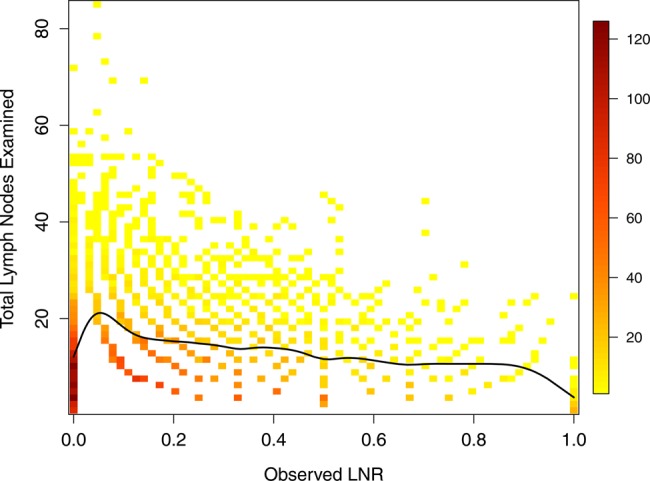
Scatter plot of total lymph nodes examined (TLN) versus observed lymph node ratio (LNR). The colors and legend represent the number of subjects at each point, and the solid line a smoothing spline fit to the TLN and LNR data points. 6174 SEER subjects in the analysis dataset had at least one examined node and are included in the plot.

Bayesian modeling approach

A Bayesian modeling framework was developed for the prediction of LNR and survival. Bayesian modeling is characterized by its allowance of prior information, specified as prior distributions, to be formally combined with new data, through their sampling distributions, to obtain a posterior distribution from which probability statements can be made about all model parameters. The parameters of particular interest in this study are the true, but unobserved, LNRs. In our Bayesian approach, these are simultaneously modeled with logistic regression and included as predictors in a Cox regression model for overall survival. Modeling details are provided in the following sections. Inclusion of prior information is an advantage of the approach, as are its ability to accommodate the complex, hierarchical model and provide realistic prediction errors. Conversely, model complexities require that the posterior distribution be estimated with computationally intensive simulation methods.

Lymph node ratio model

At cancer diagnosis, patient lymph nodes are often biopsied to test for evidence of disease spread. Previous studies have observed associations between the percentages of PN (LNR) and clinical outcomes, and there is increasing interest in LNR as a prognostic marker. However, the number of nodes biopsied is relatively small and can vary from patient to patient. Accordingly, the observed LNR merely provides an estimate of the true proportion positive among all nodes. Such estimates will be more precise in patients with larger numbers of biopsied nodes (total lymph nodes, TLN). Thus, statistical analyses of LNR should account for differences in TLN. Moreover, there may be other clinicopathologic factors associated with LNR that could be utilized to increase precision in its estimation. This section presents a statistical model that accounts for TLN and incorporates other factors in the estimation of LNR.

Our approach is a logistic regression model for the true proportions of positive lymph nodes in patients . In particular, the observed numbers of PN are assumed to have conditionally independent binomial distributions with probabilities and sample sizes equal to the total numbers of examined nodes. The logit of the probability is, in turn, defined to be a linear combination of predictors and normally-distributed random effects . Letting denote a dataset containing the observed sample sizes and predictors, and the unknown model parameters; the data contribution in analyses is in the form of the sampling distribution

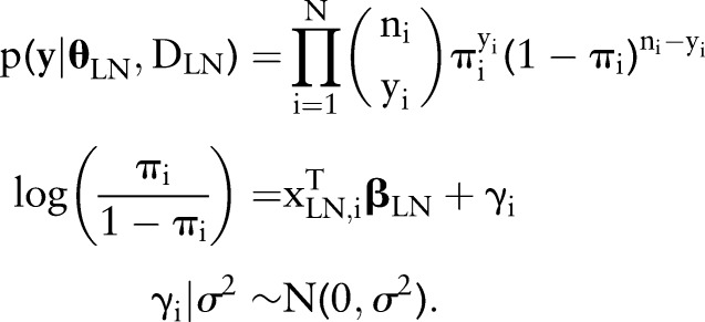Systematic LNR differences across values of the predictors are captured by the effects, and between-patient variance with . To reflect a lack of prior information in this part of the Bayesian model, the following vague prior distributions are specified:

Results from the logistic model will be summarized with , computed at clinically meaningful changes in the predictors, and with the predictive distribution of at subject-specific values of the predictors.

Survival model

Unlike other studies that have examined the effect of observed LNR on clinical outcomes, we study the effect of true LNR directly. In particular, a unified modeling approach is taken in which true LNR and its effect on overall survival are estimated simultaneously. Advantages of the approach include more accurate prediction errors, utilization of all data sources (biopsy, predictors, and survival) for LNR estimation, and accommodations for patients without biopsied nodes. An added advantage of our treatment of LNR is that we model the continuous functional form of its effect on survival.

Our analysis approach for overall survival, defined as time from diagnosis to death or censoring, is based on the Cox regression model of the general form

in which rate of death from any cause is equal to a population-specific hazard rate times multiplicative effects of subject-specific predictors x and coefficients β. Following the model formulation of Kalbfleisch¹⁰ and Ibrahim et al,¹¹ a semi-parametric Bayesian approach is used in the analysis. Given below is the sampling distribution of observed follow-up times , death indicators , and dataset of predictor variables ; conditional on unknown model parameters . Indicator functions return a value of 1 if A is true and 0 otherwise. Model terms are the unique death times, augmented with and . Parameter denotes the incremental change in the cumulative baseline hazard in time interval j, are the logistic-modeled LNR parameters defined previously, and is an arbitrary set of basis functions (eg, polynomials, splines, categorical indicators) with which to model the LNR effect.

Intuitively, each term in the product above represents the probability of patient i remaining alive at the end of his or her follow-up period if censored , and the probability of dying otherwise. Their product is thus the probability of the set of observed survival outcomes, conditional on the model parameters. Prior distributions on the parameters are specified as

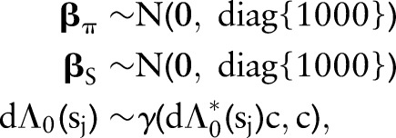where has a prior mean and variance . We model the prior mean as having an exponential distribution with rate parameter r so that . Elicitation of prior information is more naturally obtained for the cumulative survival function , where

The choice of an exponential distribution for induces a gamma prior on the cumulative hazard with the same exponential distribution mean; namely,

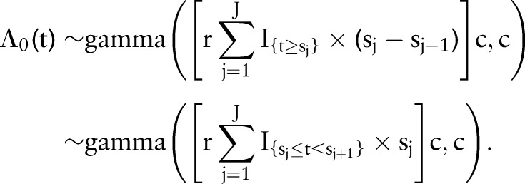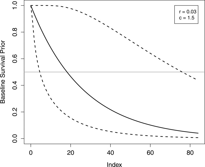
Since the cumulative survival function is simply a transformation of the cumulative hazard, values of hyperparameters r and c can be chosen to reflect prior information about baseline survival. In the proportional hazards model being fit, the baseline survival function represents the reference group of subjects whose predictor variables all equal zero. To facilitate specification of the prior, variables were coded to set the reference group at the mean and modal values of continuous and categorical predictor variables, respectively. Accordingly, we set r=0.03 and c=1.5 to specify a prior distribution with median survival time having a mean of 18 months and a 0.05–0.95 quantile range of 4–76 months (figure 2), which reflect median survival among the reference group of patients at our institution and our uncertainty in the survival function.

Figure 2.

Mean (solid line) and 90% probability intervals (dashed lines) for the prior distribution induced on the baseline hazard function.

Results from our survival analysis will be summarized with for clinically meaningful changes in the predictors and with cumulative survival functions at select values of the predictors.

Posterior simulation

The LNR and survival models, described previously and summarized in online supplementary figure S1, are fit simultaneously as a single hierarchical model in the Bayesian approach. Inference is then based on the joint posterior distribution of all model parameters, given the data; which is proportional to the product of the sampling and prior distributions, as given below.

Since the posterior is of a complicated form for which inference cannot be made directly, Markov chain Monte Carlo methods were employed to simulate samples from the posterior. In particular, the Stan software¹² was used for model implementation and simulation. To assess convergence of samples to the posterior, parallel chains were simulated with different starting values and evaluated with the multivariate potential scale reduction factor of Brooks and Gelman¹³ as provided by the ‘coda’ R package.¹⁴

Final results of the SEER data analysis will be summarized with posterior means and 95% highest posterior density intervals (PI) computed with the method of Chen and Shao.¹⁵ Monte Carlo standard errors (SEs) (MCSEs) will be reported as measures of simulation errors in posterior mean estimates.

Model diagnostics and predictive performance

The SEER data were divided randomly into a training set containing two-thirds of the patients and a validation set containing the other third. Variable selection, model parameter estimation, and goodness-of-fit diagnostics were performed with the training set. The validation set was used to assess the predictive performance of the model developed with the training set. Different biologically relevant combinations of variables were considered for inclusion in the model, with the final choice being made so as to minimize the deviance information criterion (DIC)¹⁶ and to assure adequate model fit. As global assessments of fit, posterior predictive p values¹⁷ were computed for each of the LNR and survival models using Pearson’s χ²-based goodness-of-fit statistics of the form

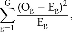where the summation is over patients partitioned into G groups according to equally-sized quantiles of and , respectively. The observed outcomes are group-specific numbers of positive lymph nodes and deaths , and the expected outcomes are predicted numbers and , respectively. Patients were partitioned into G=100 groups for analysis of the large SEER dataset. A posterior p value represents the probability that future data from the model will have a test statistic value greater than that of the observed data. Resulting values close to 0 or 1 are indicative of a lack-of-fit; values equal to 0.5 provide no evidence of lack-of-fit.

To evaluate prediction accuracy, we first simulated the predictive LNR and survival distributions individually for each patient in the validation set, using the posterior distribution of the model parameters obtained from the training set. The c (concordance) index, as described by Heagerty and Zheng¹⁸ and supplied by the ‘Hmisc’ R package,¹⁹ was then calculated as a measure of agreement between predicted and observed survival. Since the index is a commonly reported measure of predictive performance, we provide it for our model to facilitate comparisons with other published modeling efforts. It can be interpreted as the probability that, among a pair of randomly selected patients, death occurs sooner for the one with smaller predicted survival, and thus is similar to area under the receiver operating characteristic curve.²⁰ In general, a c index value of 0.5 indicates chance agreement between survival prediction and observed death outcomes, and 1.0 indicates perfect agreement.

Interactive web application

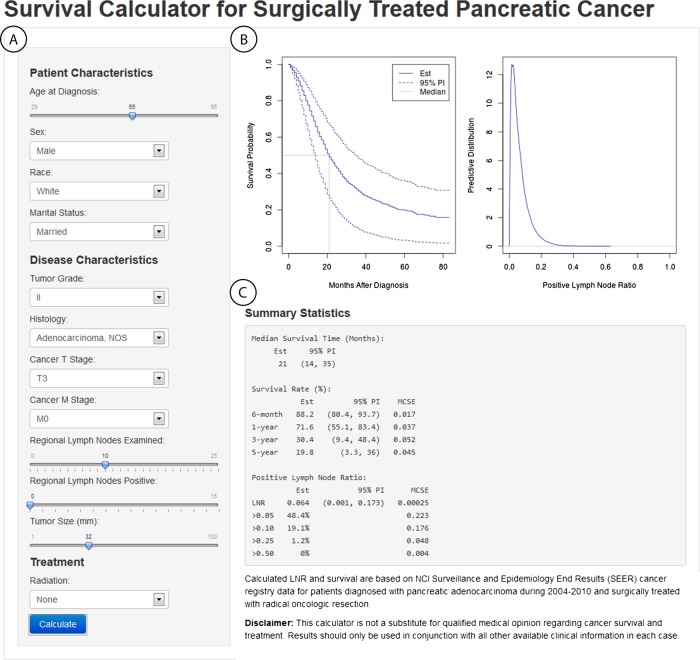
A web application was developed with the ‘shiny’ R package²¹ to provide a point-and-click interface for inputting patient baseline information and displaying resulting posterior predicted survival and LNR from our model. The application is available online at http://www.myweb.uiowa.edu/bjsmith/pancreas/. The main components of the interface are shown in the figure 3 screenshot and described below.

1. Sidebar panel: interactive widgets for user inputting of information on a new patient for which posterior survival and LNR prediction is desired.

2. Plot output panel: plots of the posterior survival function mean and prediction interval, posterior mean of the median survival time, and a kernel-density smoothed estimate of the posterior predictive distribution of LNR.

3. Text output panel: corresponding estimates of median, 6-month, and yearly survival; predicted LNR; and probabilities of LNR >0.05, 0.10, 0.25, and 0.50.

Figure 3.

Interactive web application for posterior inference. (A) provides interactive widgets for the inputting of patient and disease characteristics, (B) displays the predicted survival curve and distribution for true lymph node ratio (LNR) status, and (C) gives corresponding estimates for median and time-specific survival, and for LNR and its probabilities of being >0.05, 0.10, 0.25, and 0.50.

Implementation of the web application was accomplished entirely with R functions provided by the shiny package and required no additional use of other programming languages, such as java or HTML. Consequently, sidebar input can be passed seamlessly to the R implementation of our model, and posterior results passed back to the plot and text output panels.

Results

SEER model development

Tables 1 and 2 list the biologically relevant SEER predictor variables that were considered for inclusion in the prognostic model. Effects of numerical variables were modeled with natural cubic splines, and categorical effects with indicator variables. An initial model was fit with all variables included in the set of survival predictors and with grade, stage (T and M), and tumor size in the LNR set. Tumor site was removed from the survival set in a backward variable elimination step, since it did not improve model fit, as measured by DIC. The resulting final model included the predictors shown in figure 4. Through the joint modeling of LNR and survival, three sources of data inform on each of the components. Specifically, information on LNR status comes from observed predictor variables, examined nodes, and survival outcomes through the inclusion of LNR in the survival model. Likewise, survival is modeled as a function of observed predictors, predicted LNR, and survival outcomes. Consequently, information in the data is more fully utilized in our approach than in other methods that model LNR and survival separately.

Figure 4.

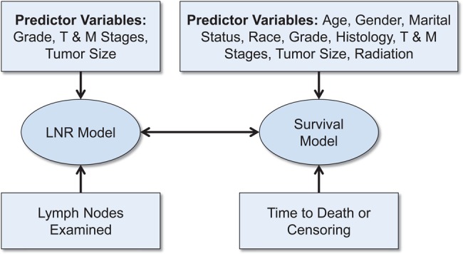
Relationships between the final lymph node ratio and survival models and the data that inform on them.

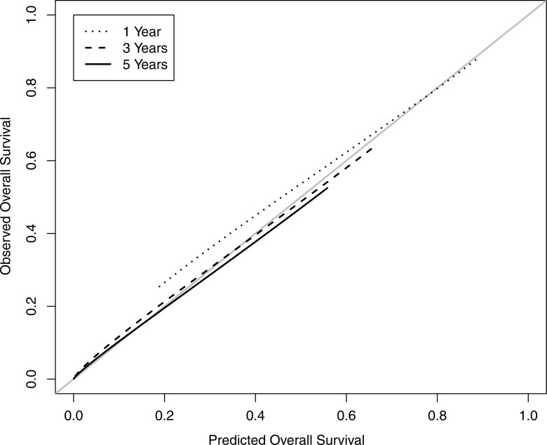
Model fit was tested with the goodness-of-fit statistics described previously. Posterior p values for the final model provided no significant evidence of lack-of-fit (LNR: p=0.3300; survival: p=0.4847). The concordance index for the predictive performance is 0.65 (95% CI 0.63 to 0.66). A few studies have developed prognostic models for pancreatic patient cohorts similar to ours. Among those, a model by Brennan et al²² produced a concordance index of 0.64 when trained and validated with patients from their institution. Since their model contains predictors not available in SEER, it cannot be validated with our data. Katz et al²³ present a prognostic model that yields a concordance index of 0.62 (95% CI 0.58 to 0.65) when applied to our validation data. Thus, the predictive performance of our model compares favorably to previous efforts. Additional model calibration was performed to compare 1-, 3-, and 5-year predicted and observed survival in the validation set, using the ‘rms’ R package.²⁴ Results are displayed in figure 5 and show excellent agreement. Finally, a sensitivity analysis was performed in which no practical differences in inference were observed between our choice of priors and priors with variances increased by a factor of 10.

Figure 5.

Calibration of the hierarchical Bayesian lymph node ratio and survival model comparing 1-, 3-, and 5-year predicted overall survival to observed survival in the validation dataset.

Lymph node ratio

Histologic grade, T and M cancer stages, and tumor size were found to be important predictors of lymph node status and thus were included in the final LNR model. Our model, in turn, provides the predictive distribution for nodal status at given values of the predictors. An example is provided in figure 3, where the predictive distribution is shown in the upper right panel for a patient with 0 PN out of 10 examined, grade II and T3/M0 stage cancer, and a tumor size of 32 mm. From the distribution, probability statements can be made about the patient’s true LNR status. For instance, the ‘Summary Statistics’ section of the figure shows that the probabilities of having LNR greater than 0.05, 0.10, and 0.25 are 48%, 19%, and 1%, respectively. The posterior mean estimate of 0.064 is also reported as a point estimate, along with a prediction interval of (0.001, 0.173) that can be interpreted as containing the true value with 95% probability.

Our statistical model produces predictive distributions that vary across patients. For the included variables, predicted odds of PN tend to increase with increasing grade, T and M stages, and tumor size (table 3). Likewise, predicted LNR will be increased when the observed proportion is higher. Furthermore, increased numbers of nodes examined will decrease variability in the distribution and increase precision in point estimates. Consequently, another use of our model and web application is to explore the total number of nodes that should be examined to ensure a desired level of precision in inference about true LNR. For example, an important clinical question to answer is how many nodes should be examined to have a high degree of confidence that there is no nodal involvement. For the patient in figure 3 with 0 out of 10 PN, there is a 48% probability of nodal involvement (LNR >0.05). By changing the patient inputs in the web application (not shown), one can determine that the probability decreases to 39/31% if the total nodes is increased to 15/20 and the number positive is held at 0. In general, predicted LNR status will vary with both the number of nodes examined and disease characteristics, and our methods provide the tools to account for both.

Table 3.

Estimated ORs for the effects of predictors on positive lymph node probability

Variable	Levels	OR* (95% PI)
Grade	I	0.79 (0.65–0.94)
	II	1.0
	III	1.18 (1.05–1.31)
	IV	1.42 (0.74–2.20)
	Unknown	0.62 (0.48–0.77)
T stage	T1	0.32 (0.24–0.41)
	T2	0.52 (0.44–0.60)
	T3	1.0
	T4	0.79 (0.61–0.98)
M stage	M0	1.0
	M1	1.95 (1.55–2.36)
	MX	1.20 (0.61–1.87)
Tumor size (mm)	0	1.0
	50	1.69 (1.38–2.00)
	100	2.46 (1.71–3.24)

*OR estimates of positive nodes from multivariable analysis (MCSE ≤0.001).

MCSE, Monte Carlo SE; PI, posterior density intervals.

Survival

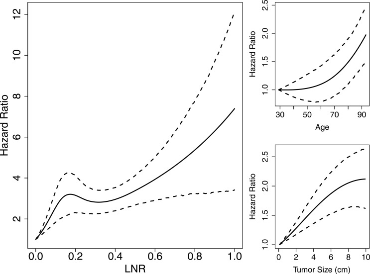
The variables found to be important predictors of survival and included in the final model are listed in figure 4. HR estimates and 95% prediction intervals are given in tables 1 and 2 for categorical variables and in figure 6 for numerical variables. True LNR as modeled by the response probability in the logistic model and included as a predictor in the survival model was found to have a strong, non-linear effect on survival (figure 6, left panel). Its estimated HR is notably increasing up to a value of 3.2 (95% PI 2.2–4.3) at an LNR of 0.17 with attenuated increases and greater uncertainty thereafter. The narrower prediction intervals at lower values of LNR reflect the larger numbers of patients at that end of the spectrum. Other notable trends are the increased risk of death for ages at diagnosis occurring primarily after 60 years, and decreased risk for those receiving radiation before (HR=0.68, 95% PI 0.52–0.85) or after (HR=0.74, 95% PI 0.68–0.80) surgery.

Figure 6.

Posterior means and 95% prediction intervals for numerical survival predictors (Monte Carlo SE (MCSE) ≤0.01).

Discussion

Our new methods for the prediction of LNR and survival offer several advancements over previous methods. First, the Bayesian approach allows for incorporation of prior information about predictor effects and population survival. The quest to understand disease processes and outcomes is often an iterative process of updating existing knowledge with new data, and the Bayesian paradigm provides a formal way to combine the two. Second, prediction is improved. Because there is a relationship between LNR and survival, joint modeling of the two utilizes more sources of information than the separate modeling employed by others. Additionally, the resulting prediction intervals are more realistic because they reflect the differences in nodes examined and uncertainty in estimating all model parameters. Joint modeling can result in an overlap of predictors between the two models, which is the case in our analysis where grade, M stage, T stage, and tumor size are significant predictors in the LNR model and significant predictors in the survival model which adjusts for LNR. This implies that LNR is related to the four predictors but does not fully account for their effect on survival. Third, splines are used to model the functional form of the LNR survival effect. This is in contrast to common alternatives in which LNR is categorized, which results in loss of information, or assumed to have a linear effect. Finally, an easily accessible web interface is provided for prediction.

In this work, our methods are applied to the latest SEER data to develop a new prognostic model for pancreatic cancer. Use of SEER data has both advantages and disadvantages. Advantages include the availability of large patient numbers, inclusion of patients across the USA, standardized collection and formatting of data, and public availability of data. Moreover, for the purposes of illustrating our methods, SEER is a familiar data source from which predictions can be generalized to a wide pancreatic cancer patient population. Limited patient-specific information, however, is a disadvantage of SEER. Genetic screening and medical imaging are sources of potential predictors that would be of interest in prognostic models but are not available currently from SEER. Some large-scale efforts are underway to make such data available, including the National Center for Biotechnology Information (NCBI) Gene Expression Omnibus (GEO),²⁵ NCI Cancer Genome Atlas (TCGA),²⁶ and NCI Quantitative Imaging Network (QIN),²⁷ although data from these are often unlinked. Rich datasets can be found at single institutions, but tend to be smaller and less generalizable. Nevertheless, we are encouraged that the predictive performance of our SEER-based model is on a par with those developed with more patient-specific information, and are eager to apply our methods to datasets with more individualized predictors.

Finally, predictions from our model can be obtained with the supplied web application. Through this interface, model results are communicated intuitively to users without the need to understand the computational and statistical complexities involved. However, some direction on the usage of this prognostic tool is in order. We envision the tool being used primarily by clinical practitioners and patients in consultation with their healthcare providers. Its survival and LNR predictions can be viewed as information akin to that provided by a published research study, albeit delivered in a more dynamic fashion. As such, users should pay particular attention to resulting prediction intervals and not focus solely on individual point estimates. The extent to which the SEER data inform on the predictions is reflected in the widths of the prediction intervals. More informative data produce narrower intervals. Thus, the widths should be taken into account when weighing results from the prognostic tool with clinical experience and other patient-specific information. In general, little is known about the effect of tools like this on clinical practice, and more research on this topic will be needed as they become more widely used.

Conclusion

Prognostic models are important aids in the understanding and treatment of disease. In this paper, we presented a new modeling framework for the prediction of LNR and survival in cancer patients. The framework was applied to a large cohort of SEER pancreatic cancer patients to produce a prognostic model and interactive web interface. These prognostic tools provide insight into patient-specific nodal status and survival. Furthermore, the framework is general and can be applied to other cancer types and datasets, with source code developed by and available from the corresponding author on request.

References

- 1.Geer RJ, Brennan MF. Prognostic indicators for survival after resection of pancreatic adenocarcinoma. Am J Surg 1993;165:68–73 [DOI] [PubMed] [Google Scholar]
- 2.Slidell MB, Chang DC, Cameron JL, et al. Impact of total lymph node count and lymph node ratio on staging and survival after pancreatectomy for pancreatic adenocarcinoma: a large, population-based analysis. Ann Surg Oncol 2008;15:165–74 [DOI] [PubMed] [Google Scholar]
- 3.House MG, Gönen M, Jarnagin WR, et al. Prognostic significance of pathologic nodal status in patients with resected pancreatic cancer. J Gastrointest Surg 2007;11:1549–55 [DOI] [PubMed] [Google Scholar]
- 4.Huebner M, Kendrick M, Reid-Lombardo KM, et al. Number of lymph nodes evaluated: prognostic value in pancreatic adenocarcinoma. J Gastrointest Surg 2012;16:920–6 [DOI] [PubMed] [Google Scholar]
- 5.Valsangkar NP, Bush DM, Michaelson JS, et al. N0/N1, PNL, or LNR? The effect of lymph node number on accurate survival prediction in pancreatic ductal adenocarcinoma. J Gastrointest Surg 2013;17:257–66 [DOI] [PMC free article] [PubMed] [Google Scholar]
- 6.Siegel R, Naishadham D, Jemal A. Cancer statistics. CA-Cancer J Clin 2013;63:11–30 [DOI] [PubMed] [Google Scholar]
- 7.Banks J. Nomograms. In: Kotz S, Read CB, Balakrishnan N, Vidakovic B. eds. Encyclopedia of statistical sciences. 2nd edn Vol 8 New York, NY: Wiley, 2005:5531–7 [Google Scholar]
- 8.Surveillance, Epidemiology, and End Results (SEER) Program. SEER*Stat database: incidence—SEER 18 regs research data + hurricane Katrina impacted Louisiana cases, Nov 2012 sub (1973–2010 varying)—linked to county attributes—total U.S., 1969–2011 Counties. National Cancer Institute, DCCPS, Surveillance Research Program, Surveillance Systems Branch. Released April 2013, based on the November 2012 submission
- 9.Collaborative Stage Work Group of the American Joint Committee on Cancer. Collaborative stage data collection system user documentation and coding instructions, version 02.03.02. Chicago, IL: American Joint Committee on Cancer, 2011 [Google Scholar]
- 10.Kalbfleish JD. Nonparametric Bayesian analysis of survival time data. J R Stat Soc B 1978;40:214–21 [Google Scholar]
- 11.Ibrahim JG, Chen M-H, Sinha D. Bayesian survival analysis. In: Armitage P, Colton T. eds. Encyclopedia of biostatistics. Wiley; Published Online: 15 Jul 2005. 10.1002/0470011815.b2a11006 [Google Scholar]
- 12.Stan Development Team. Stan: a C++ library for probability sampling, version 1.3.0. http://mc-stan.org/ (accessed 21 Jun 2013)
- 13.Brooks S, Gelman A. General methods for monitoring convergence of iterative simulations. J Comp Graph Stat 1998;7:434–55 [Google Scholar]
- 14.Plummer M, Best N, Cowles K, et al. CODA: convergence diagnostics and output analysis for MCMC. R News 2006;6:7–11 [Google Scholar]
- 15.Chen M-H, Shao Q-M. Monte Carlo estimation of Bayesian credible and HPD intervals. J Comp Graph Stat 1999;8:69–92 [Google Scholar]
- 16.Spiegelhalter DJ, Best NG, Carlin BP, et al. A Bayesian measures of model complexity and fit (with discussion). J R Statist Soc B 2002;64:583–639 [Google Scholar]
- 17.Gelman A, Meng X-L, Stern H. Posterior predictive assessment of model fitness via realized discrepancies. Stat Sinica 1996;6:733–807 [Google Scholar]
- 18.Heagerty PJ, Zheng Y. Survival model predictive accuracy and ROC curves. Biometrics 2005;61:92–105 [DOI] [PubMed] [Google Scholar]
- 19.Harrell FE. Hmisc: Harrel miscellaneous, version 0.3.10. http://cran.r-project.org/package=Hmisc (accessed 21 Jun 2013)
- 20.Hanley JA, McNei BJ. The meaning and use of the area under a receiver operating characteristic (ROC) curve. Radiology 1982;143:29–36 [DOI] [PubMed] [Google Scholar]
- 21.RStudio, Inc. Shiny: web application framework for R, version 0.6.0. http://cran.r-project.org/package=shiny (accessed 21 Jun 2013)
- 22.Brennan MF, Kattan MW, Kilmstra D, et al. Prognostic nomogram for patients undergoing resection for adenocarcinoma of the pancreas. Ann Surg 2004;240:293–8 [DOI] [PMC free article] [PubMed] [Google Scholar]
- 23.Katz MHG, Hu C-Y, Fleming JB, et al. Clinical calculator of conditional survival estimates for resected and unresected survivors of pancreatic cancer. Arch Surg 2012;147:513–19 [DOI] [PMC free article] [PubMed] [Google Scholar]
- 24.Harrell FE. Regression modeling strategies: with applications to linear models, logistic regression, and survival analysis. New York, NY: Springer-Verlag, 2001 [Google Scholar]
- 25.Barrett T, Wilhite SE, Ledoux P, et al. NCBI GEO: archive for functional genomics data sets-update. Nucleic Acids Res 2013;41(database issue):D991–5 [DOI] [PMC free article] [PubMed] [Google Scholar]
- 26.NCI. The Cancer Genome Atlas Research Network. http://cancergenome.nih.gov/ (accessed 21 Jun 2013)
- 27.NCI. Quantitative imaging for evaluation of responses to cancer therapies. http://imaging.cancer.gov/programsandresources/specializedinitiatives/qin/ (accessed 21 Jun 2013)
Associated Data
This section collects any data citations, data availability statements, or supplementary materials included in this article.