A Flexible Spatio-Temporal Model for Air Pollution with Spatial and Spatio-Temporal Covariates

Abstract

The development of models that provide accurate spatio-temporal predictions of ambient air pollution at small spatial scales is of great importance for the assessment of potential health effects of air pollution. Here we present a spatio-temporal framework that predicts ambient air pollution by combining data from several different monitoring networks and deterministic air pollution model(s) with geographic information system (GIS) covariates. The model presented in this paper has been implemented in an R package, SpatioTemporal, available on CRAN.

The model is used by the EPA funded Multi-Ethnic Study of Atherosclerosis and Air Pollution (MESA Air) to produce estimates of ambient air pollution; MESA Air uses the estimates to investigate the relationship between chronic exposure to air pollution and cardiovascular disease. In this paper we use the model to predict long-term average concentrations of NO_x in the Los Angeles area during a ten year period. Predictions are based on measurements from the EPA Air Quality System, MESA Air specific monitoring, and output from a source dispersion model for traffic related air pollution (Caline3QHCR). Accuracy in predicting long-term average concentrations is evaluated using an elaborate cross-validation setup that accounts for a sparse spatio-temporal sampling pattern in the data, and adjusts for temporal effects. The predictive ability of the model is good with cross-validated R² of approximately 0.7 at subject sites.

Replacing four geographic covariate indicators of traffic density with the Caline3QHCR dispersion model output resulted in very similar prediction accuracy from a more parsimonious and more interpretable model. Adding traffic-related geographic covariates to the model that included Caline3QHCR did not further improve the prediction accuracy.

1 Introduction

The Multi-Ethnic Study of Atherosclerosis and Air Pollution (MESA Air) is a cohort study funded by the Environmental Protection Agency (EPA) with the aim of assessing the relationship between chronic exposure to air pollution and the progression of sub-clinical cardiovascular disease (Kaufman et al, 2012). Early cohort studies of associations between exposure to air pollution and health outcomes assigned exposure based on area-wide monitored concentrations in different geographic regions (Dockery et al, 1993; Pope et al, 2002). More recent studies have used individual exposure estimates based on various spatial interpolation techniques (Brauer et al, 2003; Basu et al, 2000; Jerrett et al, 2005; Miller et al, 2007; Hoek et al, 2008; Puett et al, 2009).

One possible source of bias in air pollution cohort studies is uncontrolled spatial confounding at a regional scale. Since it is only possible to adjust for spatial confounding at a scale that is coarser than the scale of spatial variability in the predicted exposure surface (Paciorek, 2010), improved spatial predictions that provide exposure estimates with intra-urban variability enable us to reduce bias by adjusting for confounding at a regional scale. Furthermore, spatial prediction errors need to be treated as measurement error in the health effect analysis (Szpiro et al, 2011b; Sheppard et al, 2012; Gryparis et al, 2009; Carroll et al, 2006), and accurate spatial prediction at a fine scale can reduce this measurement error, potentially decreasing bias and increasing precision. Thus, subject-specific exposures provide greater heterogeneity in the exposure estimates, improving the health effect studies by 1) increasing study power; 2) reducing measurement error from predicted exposures; and 3) allowing us to control for confounding by region.

A primary focus of the MESA Air study is the development of accurate predictions of ambient air pollution at the home locations of study participants (Bild et al, 2002; Kaufman et al, 2012). The MESA Air study includes gaseous oxides of nitrogen (NO_x), particulate matter with aerodynamic diameter less than 2.5 μm (PM_2.5), as well as other gaseous co-pollutants in six major US metropolitan areas: Los Angeles, CA; New York, NY; Chicago, IL; Minneapolis-St. Paul, MN; Winston-Salem, NC; and Baltimore, MD. In this paper we use 10 years of MESA Air ambient NO_x data from the Los Angeles region for estimation and evaluation of a spatio-temporal model.

Our observations of ambient outdoor NO_x concentrations in Los Angeles consist of both EPA Air Quality System (AQS) regulatory monitoring and MESA Air supplemental monitoring (for details of the MESA Air data-set, see Cohen et al, 2009; Szpiro et al, 2010; Sampson et al, 2011). The supplementary monitoring campaign was designed to provide increased geographic diversity, specifically w.r.t proximity to traffic and sampling near participant homes. To match the 2-week timescale of the supplementary MESA Air monitoring, the AQS data was aggregated to 2-week averages (missing data handled as in Szpiro et al, 2010); to account for skewness the resulting 2-week average NO_x concentrations were log-transformed.

The observation locations fall into three general groups: 1) Fixed sites — AQS and MESA Air sites that that provide long time series of 2-week averages at a few fixed locations; 2) Home (outdoor) sites — a rotating set of four monitors, placed at a subset (roughly 10%) of participant home locations, collecting at least two 2-week averages at each site; 3) Community snapshot — simultaneous measurements at a large number of locations, including roadway gradients, for three 2-week periods during different seasons. The roadway gradients consisted of six monitors placed perpendicular to major roadways, three on either side, at distances of approximately 30, 100, and 250 meters. A summary of available data, including the location of monitors and examples of time-series, can be found in Tables 1–2 and Figures 1–3.

Table 1.

Summary of observations used for modeling

Type of site	No. of sites	Start date	End date	No. of measurement
AQS	20	1999–01–13	2009–09–23	4178
MESA fixed	5	2005–12–07	2009-07-01	399
MESA home	84	2006–05–24	2008–02–13	155
MESA snapshot1	177	2006–07–05	2007–01–31	449

¹Snapshot measurements where carried out during three 2-week periods centered on the Wednesdays of 2006–07–05, 2006–10–25, and 2007–01–31

Table 2.

Summary statistics for the data, both on the original ppb scale and on the logscale. The variability in the mean between the three snapshots is due to the seasonal patterns in NO_x.

	ppb NOx		log(ppb NOx)
	Mean	Std.	Mean	Std.
AQS and MESA fixed
2-week	55.5	39.9	3.77	0.724
long-term avg.	56.0	18.4	3.77	0.394
Snapshot
2006–07–05	34.2	11.5	3.47	0.387
2006–10–25	75.1	23.5	4.27	0.317
2007–01–31	95.3	27.0	4.51	0.299
Home sites	45.6	28.3	3.63	0.642

Figure 1.

Schematic image of the data available for analysis. Each measurement is represented by a point in space and time. AQS provides temporally rich observations at 20 locations. During the second half of our modeling period, additional temporally rich data are provided by 5 MESA fixed sites. Spatial data are provided by the three MESA snapshot campaigns, which monitored a total of 177 locations at three time points, and by MESA home sites that consists of four monitors alternating among 84 locations.

Figure 3.

Example time series of log-transformed 2-week average NO_x concentrations at three AQS monitors and one home site in the Los Angeles area. The fit of our smooth temporal basis functions to the data, and the transformed Caline predictions are also shown. For the home site we have used the smooth temporal fit at the closest AQS monitor.

Several general overviews of statistical modeling approaches for spatially and spatio-temporally correlated data exist (Banerjee et al, 2004; Cressie and Wikle, 2011), including non-separable spatio-temporal covariance functions (Gneiting and Guttorp, 2010) and dynamic model formulations (Gamerman, 2010). There are also several methods developed specifically for the modeling of air pollution data (Smith et al, 2003; Sahu et al, 2006; Calder, 2008; Fanshawe et al, 2008; Paciorek et al, 2009; De Iaco and Posa, 2012). However, these methods either require relatively complete observation matrices, or do not allow for sufficiently complex spatio-temporal dependencies. Additionaly, the methods are often developed for geographic regions much larger than those of interest for MESA Air.

Here we generalize a model, previously described by Sampson et al (2011) and Szpiro et al (2010). The model uses temporal basis functions to account for the temporal variability in data. To account for spatial variability in the temporal structure (see Figure 3), the basis functions are modulated by spatially varying coefficients. The coefficients are modeled using universal kriging, where the linear trend contains Geographic Information System (GIS) covariates. The use of GIS covariates is termed “land use” regression (LUR) (Jerrett et al, 2005; Hoek et al, 2008). Covariates used for the the Los Angeles NO_x data are: 1) distance to a major road, i.e., census feature class code A1–A3 (distances truncated to be ≥ 10m and log-transformed), 2) distance to a A1 road (≥10m, log-transformed), 3) total length of A1 and A2 roads in a circular buffer with 300 meter radius, 4) total length of A3 roads in a 50 meter buffer, 5) distance to coast (truncated to be ≤ 15 km), and 6) average population density in a 2 km buffer. Here census feature class code A1 roads refer to interstates and other limited access highways; A2 are primary roads without limited access; and A3 are secondary roads, e.g. state highways (see pp. 3-27 in US Census Bureau, 2002). Available covariates are described in Cohen et al (2009); selection of covariates is presented in Mercer et al (2011). Having used spatially varying temporal basis functions to account for temporal variability (see (2) in Section 2 for details), the residuals are assumed to consist of mean zero spatially dependent, but temporaly uncorrelated fields (Sampson et al, 2011; Szpiro et al, 2010).

Deterministic numerical models that provide predictions of air pollution offer an alternative to statistical modeling (Appel et al, 2008). However, comparisons between measurements and air quality model output show varied prediction performance (Appel et al, 2008; Hogrefe et al, 2006), and an alternative is to combine model output with observations. In contrast to existing studies (Fuentes and Raftery, 2005; Berrocal et al, 2010), which combine observations with output from grid-based models, we have here opted to combine our observations with the output from a point prediction model (Caline3QHCR, Eckhoff and Braverman, 1995, hereafter called Caline). Given locations of major sources and local meteorology Caline uses a dispersion model to predict how nonreactive pollutants travel with the wind, providing hourly estimates of air pollution at distinct points. The Caline predictions used here are based on estimates of traffic density on major roads in the Los Angeles area (see Wilton et al, 2010; Lindström et al, 2011, for details).

The main contributions of this paper are: 1) extending the model presented in Szpiro et al (2010) to include spatio-temporal covariates; 2) applying the model to the MESA Air NO_x dataset to generate predictions for Los Angeles; 3) evaluating the model’s ability to predict long term averages using a cross-validation strategy that accounts for the complex MESA Air monitoring design and that allows us focus on spatial predictive ability by accounting for temporal effects; 4) investigating the benefit of Caline as a spatio-temporal covariate and Caline’s ability to replace traditional LUR covariates; and 5) reducing the computational burden of the model and evaluating how the computational burden scales with the number of observations. The model presented here has been implemented in an R package, SpatioTemporal, which is available from http://cran.r-project.org/package=SpatioTemporal

The model is presented in Section 2. Computational considerations and parameter estimation are discussed in Section 3. Model validation, including considerations for the unbalanced dataset, is presented in Section 4. In Section 5 we apply the model to NO_x data from Los Angeles, and investigate the contribution from Caline. Section 6 concludes with a discussion.

2 Model

We let C(s, t) denote the observed concentration of NO_x at location s and time t and take y(s, t) = log C(s, t). N denotes the total number of observations; n the number of observation locations; and T the number of observation time points. Due to our unbalanced sampling, N ⪡ nT. Our goal is to predict concentrations at unobserved locations and/or times. We denote these unknown values by C*(s, t). For convenience important notation is summarized in Table 3.

Table 3.

Important notation and symbols

Symbol	Meaning
C(s, t)	Observed 2-week average concentrations.
C*(s, t)	Unobserved 2-week average concentrations.
y(s, t)	log C(s, t).
μ(s, t)	Mean field part of y(s, t).
ν(s, t)	Space-time residual part of y(s, t).
fi(t)	Smooth temporal basis functions.
βi(s)	Spatially varying regression coefficients, weighing the i:th temporal trends differently at each site.
Xi	Land use regression (LUR) basis functions for the spatially varying regression coefficients in βi(s).
α i	Regression coefficients for the i:th LUR-basis.
${\mathcal{M}}_l(s,t)$	Spatio-temporally varying covariates.
γl	Regression coefficient for the spatio-temporally varying covariates.
N	No. of observations.
T	No. of observed time-points.
n	No. of observed sites.
nt	No. of observations at time t. Note that $N={\sum }_{t=1}^T{n}_t$ and nt < n ∀t.
m	No. of temporal basis functions (incl. intercept).
L	No. of spatio-temporal model outputs.
pi	No. of LUR-basis functions for the i:th temporal-basis function (incl. intercept).

The spatio-temporal process is decomposed into

$$y(s,t)=\mu (s,t)+\nu (s,t),$$ (1)

where μ(s, t) is the mean process and ν(s, t) is the space-time residual process.

The mean process is modeled as

$$\mu (s,t)=\sum _{l=1}^L{\gamma }_l{\mathcal{M}}_l(s,t)+\sum _{i=1}^m{\beta }_i\left(s\right)f_i\left(t\right),$$ (2)

where ${\mathcal{M}}_l(s,t)$ are spatio-temporal covariates with coefficients ${\gamma }_l;{\left\{f_i\right(t\left)\right\}}_{i=1}^m$ is a set of smooth temporal basis functions, with f₁(t) ≡ 1 and f₂(t), …, f_m(t) having mean zero; and the β_i(s) are spatially varying coefficients for the temporal trends. Typically the number of basis functions, m, will be small. The basis functions are derived as smoothed singular vectors using observations at the fixed sites; the basis functions are treated as fixed and known for the modeling (see Fuentes et al, 2006; Szpiro et al, 2010; Sampson et al, 2011, for details).

We model the spatial fields of β_i-coefficients using universal kriging (Cressie, 1993). The trend in the kriging is constructed as a linear regression on (geographic) covariates. The spatial dependence structure is provided by a set of covariance matrices, ∑_βi(θ_i), parameterized by θ_i. The resulting models for the β-fields are

$${\beta }_i\left(s\right)\in \mathrm{N}(X_i{\alpha }_i,{\Sigma }_{{\beta }_i}({\theta }_i\left)\right)\text{for}i=1,\dots ,m,$$ (3)

where X_i are n × p_i design matrices, α_i are p_i × 1 matrices of regression coefficients, and Σ_βi(θ_i) are n × n covariance matrices. We assume the β_i(s) fields are, a priori, independent of each other.

The residual space-time process is modeled using mean zero Gaussian fields that are temporally independent, but spatially dependent

$$\nu (s,t)\in \mathrm{N}(0,{\Sigma }_{\nu }^t({\theta }_{\nu }\left)\right)\text{for}t=1,\dots ,T;$$ (4)

the size of each covariance matrix, ${\Sigma }_{\nu }^t\left({\theta }_{\nu }\right)$, is given by the numbers of observations, n_t, at time t. The covariance matrices depend on parameters, θ_ν. Note that only the number of elements in ${\Sigma }_{\nu }^t\left({\theta }_{\nu }\right)$, not the parametric functional form, varies with t. The covariance matrices in (3) and (4) are not required to share a common covariance model, allowing for a very flexible model.

The parameters of the model consist of: regression parameters for the spatio-temporal and geographic covariates, γ = (γ₁, …, γ_L)^T and $\alpha ={({\alpha }_1^{⊺},\dots ,{\alpha }_m^{⊺})}^{⊺}$; covariance parameters for the β_i-fields, θ_B = (θ₁, …, θ_m); and covariance parameters of the spatio-temporal residuals, θ_ν. To simplify notation we collect the covariance parameters into Ψ = (θ₁, …, θ_m,θ_ν).

Combining (1) and (2) our model becomes

$$y(s,t)=\sum _{l=1}^L{\gamma }_l{\mathcal{M}}_l(s,t)+\sum _{i=1}^m{\beta }_i\left(s\right)f_i\left(t\right)+\nu (s,t).$$ (5)

Following Szpiro et al (2010), we introduce the N × 1-vectors Y = y(s, t) and V = ν(s, t) by stacking the elements into single vectors varying first s and then t; a mn × 1-vector B = (β₁(s)^T, …, β_m(s)^T)^T; and a sparse N × mn-matrix F = (f_st,is’) with elements

$$f_{\mathit{st},{\mathit{is}}^{\prime }}=\{\begin{array}{cc}{f}_i\left(t\right)\hfill & s=s^{\prime }\hfill \\ 0\hfill & \text{otherwise}.\hfill \end{array}\phantom{\}}$$

To accommodate the spatio-temporal covariates we also introduce a N × L-matrix $\mathcal{M}$, with each row containing covariates for the space-time location of the corresponding row in Y. Using these matrices we rewrite (5) as

$$Y=\mathcal{M}\gamma +\mathit{FB}+V,$$ (6)

where B ∈ N (Xα,Σ_B(θ_B)) and V ∈ N (0, Σ_ν(θ_ν)); X, Σ_B(θ_B), and Σ_ν(θ_ν) are block diagonal matrices with diagonal blocks ${\left\{X_i\right\}}_{i=1}^m,{\left\{{\Sigma }_{{\beta }_i}\right({\theta }_i\left)\right\}}_{i=1}^m$, and ${\left\{{\Sigma }_{\nu }^t\right({\theta }_{\nu }\left)\right\}}_{t=1}^T$ respectively. Noting that (6) is a linear combinations of independent Gaussians we introduce the matrices

$$\tilde{X}=\left[\mathcal{M}\mathit{FX}\right]\text{and}\tilde{\Sigma }\left(\Psi \right)={\Sigma }_{\nu }\left({\theta }_{\nu }\right)+F{\Sigma }_B\left({\theta }_B\right)F^{⊺},$$ (7)

and write the distribution of Y as

$$[Y\mid \Psi ,\gamma ,\alpha ]\in \mathrm{N}\left(\tilde{X}\left[\begin{array}{c}\hfill \gamma \hfill \\ \hfill \alpha \hfill \end{array}\right],\tilde{\Sigma }\left(\Psi \right)\right).$$ (8)

3 Computational Considerations

Parameter estimates can now be obtained by maximizing the likelihood of (8), using a suitable optimisation algorithm (e.g. L-BFGS-B, see Byrd et al, 1995). However, for large datasets estimation using naïve maximum likelihood (ML) takes considerable time. There are two considerations for reducing the esimation time: 1) reducing the number of parameters, and 2) utilizing the block structure of Σ_ν(θ_ν) and Σ_B(θ_B) to reduce the computational burden.

Replacing γ and α with their generalised least squares estimates (see Lindström et al, 2011, for details) gives the profile likelihood of (8)

$$\begin{array}{cc}\hfill 2l_{\text{PROF}}(\Psi \mid Y)=& -N\log \left(2\pi \right)-\log \mid \tilde{\Sigma }\left(\Psi \right)\mid -Y^{⊺}{\tilde{\Sigma }}^{-1}\left(\Psi \right)Y\hfill \\ \hfill & +Y^{⊺}{\tilde{\Sigma }}^{-1}\left(\Psi \right)\tilde{X}{\left({\tilde{X}}^{⊺}{\tilde{\Sigma }}^{-1}\left(\Psi \right)\tilde{X}\right)}^{-1}{\tilde{X}}^{⊺}{\tilde{\Sigma }}^{-1}\left(\Psi \right)Y.\hfill \end{array}$$ (9)

To utilize the block diagonal structure of Σ_ν(θ_ν) and Σ_B(θ_B) we rewrite (9) as

$$\begin{array}{cc}\hfill 2l_{\text{PROF}}(\Psi \mid Y)=& -\log \mid {\Sigma }_{\nu }\left({\theta }_{\nu }\right)\mid -\log \mid {\Sigma }_B\left({\theta }_B\right)\mid -\log \mid {\Sigma }_{B\mid Y}^{-1}\left(\Psi \right)\mid -Y^{⊺}\widehat{\Sigma }\left(\Psi \right)Y\hfill \\ \hfill & +Y^{⊺}\widehat{\Sigma }\left(\Psi \right)\mathcal{M}{\left({\mathcal{M}}^{⊺}\widehat{\Sigma }\left(\Psi \right)\mathcal{M}\right)}^{-1}{\mathcal{M}}^{⊺}\widehat{\Sigma }\left(\Psi \right)Y+\text{const}.\hfill \end{array}$$ (10)

where const. does not depend on Ψ, and

$${\Sigma }_{B\mid Y}^{-1}\left(\Psi \right)={\Sigma }_B^{-1}\left({\theta }_B\right)+F^{⊺}{\Sigma }_{\nu }^{-1}\left({\theta }_{\nu }\right)F,$$ (11a)

$$\begin{array}{cc}\hfill {\Sigma }_{\alpha \mid Y}^{-1}\left(\Psi \right)& =X^{⊺}{\Sigma }_B^{-1}\left({\theta }_B\right)X-X^{⊺}{\Sigma }_B^{-1}\left({\theta }_B\right){\Sigma }_{B\mid Y}\left(\Psi \right){\Sigma }_B^{-1}\left({\theta }_B\right)X,\hfill \\ \hfill \widehat{\Sigma }\left(\Psi \right)& ={\Sigma }_{\nu }^{-1}\left({\theta }_{\nu }\right)-{\Sigma }_{\nu }^{-1}\left({\theta }_{\nu }\right)F{\Sigma }_{B\mid Y}\left(\Psi \right)F^{⊺}{\Sigma }_{\nu }^{-1}\left({\theta }_{\nu }\right)\hfill \end{array}$$ (11b)

$$\begin{array}{cc}\hfill -& [{\Sigma }_{\nu }^{-1}\left({\theta }_{\nu }\right)F{\Sigma }_{B\mid Y}\left(\Psi \right){\Sigma }_B^{-1}\left({\theta }_B\right)X{\Sigma }_{\alpha \mid Y}\left(\Psi \right)\phantom{]}\hfill \\ \hfill & \phantom{[}{X}^{⊺}{\Sigma }_B^{-1}\left({\theta }_B\right){\Sigma }_{B\mid Y}\left(\Psi \right)F^{⊺}{\Sigma }_{\nu }^{-1}\left({\theta }_{\nu }\right)].\hfill \end{array}$$ (11c)

Proof of equality between (9) and (10) is given in Appendix A.

At a first glance it is not obvious that (10) offers any computational advantages over (9). The matrix $\tilde{\Sigma }\left(\Psi \right)$ in (9) is a dense N × N-matrix, implying that the computational effort of calculating $\log \mid \tilde{\Sigma }\left(\Psi \right)\mid$ grows at a rate of $\mathcal{O}\left(N^3\right)$; the corresponding term in (10),

$$\log \mid {\Sigma }_{\nu }\left({\theta }_{\nu }\right)\mid +\log \mid {\Sigma }_B\left({\theta }_B\right)\mid +\log \mid {\Sigma }_{B\mid Y}^{-1}\left(\Psi \right)\mid ,$$

consists of the determinant of two block diagonal matrices and the determinant of a dense mn × nm-matrix. The computational effort for the three components scales are $\mathcal{O}\left({\sum }_t{n}_t^3\right),\mathcal{O}\left({\mathit{mn}}^3\right)$, and $\mathcal{O}\left(m^3{n}^3\right)$ For our data the term requiring $\mathcal{O}\left(m^3{n}^3\right)$ computer time will be the most time consuming. Due to the long time period covered and the few temporal basis functions needed we have mn ⪡ N, implying that (10) should be considerably faster to evaluate than (9). With a more balanced sampling design the term requiring $\mathcal{O}\left({\sum }_t{n}_t^3\right)$ is likely to dominate. Since ${\sum }_t{n}_t^3<{\left({\sum }_t{n}_t\right)}^3=N^3$, (10) is still faster to evaluate than (9). Similar arguments can be made for the rest of the terms in the log-likelihood, and the overall computational cost of (9) grows as $\mathcal{O}\left(N^3\right)$, compared to $\mathcal{O}\left(m^3{n}^3\right)$ or $\mathcal{O}\left({\sum }_t{n}_t^3\right)$ for (10). As an example, evaluating the likelihood once for our 5181 measurements in Los Angeles takes 92 seconds using (9), compared to 2.5 seconds for (10) (using an Intel Xeon E5410 processor). A comparison of evaluation times is presented in Figure 4. The Figure illustrates the slower increase in evaluation time as a function of the number of observations for (10) compared to (9); it also shows the “jumps” in evaluation time for (10) when the number of locations increase.

Figure 4.

Comparison of the time needed for one evaluation of the naïve profile likelihood (9) and simplified version (10). The full dataset, 5182 observations from 286 locations and 280 time points, was divided into smaller pieces by dropping either locations and/or time-points to examine how fast the evaluation time would grow as the dataset was expanded. Evaluation time for the full likelihood grows as N^2.8 (the fitted line) close to the expected theoretical value of $\mathcal{O}\left(N^3\right)$. For a fixed number of locations evaluation time for the simplified version grows considerably slower than N³.

The model (5) can also been seen as a multi-level mixed effects model (see e.g. Ch. 2 in Pinheiro and Bates, 2009); this formulation is unlikely to offer any computational gains compared to the approach above. Alternatively, recent developments in modelling of large datasets could be used to improve computational effeciency. Examples include Gaussian Markov Random Fields (Lindgren et al, 2011), predictive process (Banerjee et al, 2008) and, fixed rank kriging (Cressie and Johannesson, 2008); these have all been extended to spatio-temporal data (Cameletti et al, 2013; Finley et al, 2012; Kang et al, 2010). However, these extensions are, essentially, time dynamical models and do not allow for the complex structure, with temporal basis functions, in (2). For composite likelihood methods (Stein et al, 2004) it is non-trivial to construct blocking strategies in space and time that account for the dependencies induced by the temporal basis functions.

4 Model Validation

Having obtained estimates for the unknown parameters the next step is to predict concentrations at unobserved locations and times. Given parameter estimates predictions and prediction uncertainties for the log-concentrations, y*(s, t), are obtained as conditional expectations and variances for a multivariate Gaussian (8). Unobserved NO_x concentrations are then obtained as C*(s, t) = exp y*(s, t), and validation is based on the NO_x-data.

We assess the predictive accuracy of our model using cross-validation, taking into account the challenges presented by the unbalanced structure of our observations. The primary interest of MESA Air is the long term average exposure, leaving us with the problem of trying to validate the spatial predictions of long term averages based, in most cases, on a few observations at each location. Only a few sites (the 25 fixed sites) have time-series long enough for us to compute long-term averages; additionally, the fixed sites have less heterogeneity in their surrounding environment but larger spatial spread than the remaining observation locations.

To make the fullest use of available data we employ three different cross-validation strategies: 1) leave-one-out cross-validation for the fixed sites, 2) 10-fold cross-validation for the community snapshots (ensuring not to split road gradients between groups); and 3) 10-fold cross-validation for the home sites. For each of the scenarios above, all remaining data are used to estimate parameters and to predict at the left out locations. Given the predictions and prediction variances we compute the coverage of 95% prediction intervals, the root mean squared error (RMSE) and the corresponding cross-validated R².

For the first cross-validation approach we validate the model by comparing predicted and observed concentrations, as well as the predicted and observed long-term average concentration at each location. The long-term averages (both true and predicted) are computed by summation over only those time points for which we have observations, followed by division by the number of terms in the sum,

$$C^{\ast }\left(s\right)=\sum _{t\in \{\tau :\exists y(s,\tau \left)\right\}}\frac{\exp \left(y^{\ast }\right(s,t\left)\right)}{\mid \{\tau :\exists y(s,\tau \left)\right\}\mid }.$$

The cross-validated R² are computed as (Szpiro et al, 2011a)

$$R^2=\max \left(0,1-\frac{{\mathrm{RMSE}}^2}{\mathrm{Var}\left(C\right(s\left)\right)}\right).$$ (12)

For the community snapshot, out-of-sample predictions are calculated by leaving out the same sites during all three seasons. However, when assessing the spatial predictive ability of our model, we compute separate RMSE and R² values for each season. This has the added benefit of providing information regarding the model’s spatial predictive ability at different times.

For the home sites our measurements are spread over both time and space, making the situation more complicated. We compute the RMSE value as usual, but for R² we compare our predictions to a few simple reference models that account for (some) temporal variability. This is done by replacing Var(C(s)) in (12) by the RMSE of the reference models. Reference models used are: 1) the spatial average at each time point based on observations at fixed sites; 2) the observation from the closest available fixed site; 3) smooth temporal trends fitted to data from the closest fixed site. We denote the three reference models as average, closest, and smooth. The resulting R²’s represent the improvement in predictions provided by our model, compared to central site or nearest neighbor schemes commonly used in epidemiology studies (Pope et al, 1995; Miller et al, 2007).

5 Los Angeles NO_x Data

We now use the model to predict ambient outdoor NO_x concentrations in Los Angeles. We also investigate whether the inclusion of Caline as a spatio-temporal covariate can, a) improve the predictions; or b) act as a replacement for the road covariates. Replacing several road covariates with a single spatio-temporal covariate simplifies the model and potentially reduces the number of unknowns. To evaluate this, four different models are examined: 1) using all geographic covariates, 2) using geographic covariates and Caline, 3) using only non-road covariates, and 4) using non-road covariates together with Caline.

Several different options for including the Caline predictions in the spatio-temporal model have been considered. Since our observations are log-transformed, a similar transformation of Caline seems reasonable. However, Caline predictions are based on the contribution from major roads so we use a log(x + 1) transformation to accommodate zero predictions at sites that are far from major roads. A second issue is that the unbalanced monitoring scheme may cause the model to emphasize Caline’s temporal predictive ability over its spatial features. The results presented here use a mean separated Caline, constructed by first computing the temporal average at each location $\overline{\mathcal{M}}\left(s\right)={\sum }_t\mathcal{M}(s,t)∕T$, where $\mathcal{M}(s,t)=\log (\text{Caline}+1)$. The average is then subtracted to create a mean-zero spatio-temporal covariate as $\tilde{\mathcal{M}}(s,t)=\mathcal{M}(s,t)-\overline{\mathcal{M}}\left(s\right)$. The average, $\overline{\mathcal{M}}\left(s\right)$, is added as a geographic covariate (a column of each X_i in (3)) and $\tilde{\mathcal{M}}(s,t)$ is used as a spatio-temporal covariate (${\mathcal{M}}_l$ in (2)), allowing us to separate Caline’s spatial and temporal contributions to the predictions. Studies with no or alternate transformations, as well as a non-mean separated Caline gave results similar to, or worse than, those presented here.

For this data we use exponential covariance functions for all covariance matrices; the covariance functions are characterized by range ϕ, partial sill σ², and nugget τ². To obtain a smooth mean field in (2) we assume that the nuggets of the β_i-fields are zero. The unknown parameters, Ψ, are estimated by maximizing (10), using the L-BFGS-B algorithm (Byrd et al, 1995) in the optim() function in R (R Development Core Team, 2008).

For the first two models cross-validation showed no improvment when including Caline (see Table 4) and most of the estimated parameters are very similar (see Table 5). out-of-sample predictions of long-term averages at the AQS and MESA fixed sites are seen in Figure 5. Figure 6 shows predictions of time-series at three fixed sites. For both models the predictive ability at MESA home sites is very good, with R² ≈ 0.9. Even after the use of a simple reference model to account for the temporal variability, the spatial predictive ability remains high, with R² ≈ 0.67 − 0.76. The lowest R² values were obtained for the summer snapshot (R² ≈ 0.52) and long-term averages (R² ≈ 0.58); the summer snapshot also had the lowest RMSE values, indicating that there is little variability to be explained. For the long-term averages, several AQS sites are far from other sites or at the edge of our area of interest (see Figure 2); we expect cross-validation at these sites to exhibit larger prediction errors than at participant home locations.

Table 4.

Cross-validation results for the models with all GIS covariates, without and with Caline. The table gives RMSE, R², and coverage for 95% predictions intervals for the out-of-sample predictions. For the Home sites the three adjusted R², showing improvement over simple temporal models, are also provided. All values are computed on the back transformed scale (ppb NO_x).

	With road covariates
	No Caline			Caline
	RMSE	R 2	cov.	RMSE	R 2	cov.
AQS and MESA fixed
2-week	17.90	0.80	0.91	18.12	0.79	0.90
long-term avg.	11.97	0.58		12.26	0.56
Snapshot
2006–07–05	7.94	0.52	0.93	7.62	0.56	0.95
2006–10–25	13.32	0.68	0.97	13.32	0.68	0.95
2007–01–31	15.69	0.66	0.99	15.77	0.66	0.98
Home sites	9.34	0.89	0.97	9.06	0.90	0.95
average		0.67			0.69
closest		0.74			0.76
smooth		0.74			0.76

Table 5.

Estimated parameters for the models with all GIS covariates: no Caline compared to Caline. Parameter values and standard errors based on the observed information matrix are given

	No Caline		Caline
	Est.	Std. err.	Est.	Std. err.
Average level
α1 — Regression coefficients
Intercept	3.78	0.174	3.42	0.207
Distance to road (log10 m)	−0.0801	0.0236	−0.0665	0.0237
Distance to A1 roads (log10 m)	−0.152	0.0323	−0.0630	0.0431
A1 & A2 in 300m buffers (km)	0.0501	0.0253	0.0315	0.0256
A3 in 50m buffers (km)	0.689	0.215	0.781	0.214
Distance to coast (km)	0.0330	0.0102	0.0318	0.00990
Population (1000/2km buffer)	0.00324	0.00117	0.00335	0.00113
Average log(Caline + 1)			0.0789	0.0259
θ1 — Covariance parameters
Log Range (log km)	1.86	0.388	1.84	0.384
Log Sill	−2.86	0.287	−2.92	0.283
1st temporal trend
α2 — Regression coefficients
Intercept	−0.793	0.139	−1.00	0.187
Distance to road (log10 m)	0.00244	0.0259	0.0137	0.0254
Distance to A1 roads (log10 m)	0.0120	0.0274	0.0715	0.0379
A1 & A2 in 300m buffers (km)	0.0437	0.0227	0.0345	0.0214
A3 in 50m buffers (km)	0.136	0.255	0.178	0.245
Distance to coast (km)	0.0221	0.00720	0.0188	0.00753
Population (1000/2km buffer)	−0.00127	0.000782	−0.000949	0.000735
Average log(Caline + 1)			0.0533	0.0227
θ2 — Covariance parameters
Log Range (log km)	2.77	0.621	3.34	0.831
Log Sill	−3.82	0.512	−3.55	0.740
2nd temporal trend
α3 — Regression coefficients
Intercept	−0.142	0.132	−0.204	0.189
Distance to road (log10 m)	0.0503	0.0333	0.0532	0.0329
Distance to A1 roads (log10 m)	−0.0430	0.0326	−0.0263	0.0479
A1 & A2 in 300m buffers (km)	−0.0310	0.0281	−0.0412	0.0264
A3 in 50m buffers (km)	0.338	0.322	0.412	0.309
Distance to coast (km)	0.0130	0.00548	0.0121	0.00581
Population (1000/2km buffer)	−0.0000833	0.000924	0.0000423	0.000896
Average log(Caline + 1)			0.0185	0.0290
θ3 — Covariance parameters
Log Range (log km)	2.40	0.646	2.68	0.724
Log Sill	−4.78	0.436	−4.70	0.515
γ Mean centered log(Caline + 1)			0.0677	0.0151
θ ν
Log Range (log km)	4.39	0.0938	4.38	0.0935
Log Sill	−3.25	0.0617	−3.25	0.0614
Log Nugget	−4.29	0.0415	−4.30	0.0418

Figure 5.

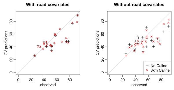
Out-of-sample predictions for the long-term averages at the AQS and MESA fixed sites. Results for the model both including the road covariates (left) and without the road covariates (right) are given; for both cases predictions without and with Caline are shown.

Figure 6.

Example of out-of-sample predictions of the log-transformed 2-week average NO_x concentrations at three AQS monitors and one home site in the Los Angeles area. Observations, predictions, and 95% prediction intervals are shown.

Figure 2.

Map illustrating the location of our measurements. The collocated AQS and MESA fixed site are north of the Lynwood AQS site; the MESA fixed site is partially obscured by the AQS sites.

For the two models (3 and 4) that excluded the GIS road covariates the model including Caline performed uniformly better in cross-validation (see Table 6 and Figure 5). In fact, predictions from model 4 are nearly comparable to those obtained with models 1 and 2. This suggests that Caline may provide an interpretable replacement for GIS road covariates.

Table 6.

Cross-validation results for the model without and with Caline, but excluding all road covariates. The table gives RMSE, R², and coverage for 95% predictions intervals for the out-of-sample predictions. For the Home sites the three adjusted R²:s, showing improvement over simple temporal models, are also provided. All values are computed on the back transformed scale (ppb NO_x)

	Without road covariates
	No Caline			Caline
	RMSE	R 2	cov.	RMSE	R 2	cov.
AQS and MESA fixed
2-week	20.42	0.74	0.91	18.40	0.79	0.92
long-term avg.	15.77	0.27		12.74	0.52
Snapshot
2006-07-05	9.68	0.29	0.93	8.26	0.48	0.95
2006-10-25	16.51	0.51	0.98	14.90	0.60	0.95
2007-01-31	20.45	0.43	0.98	18.19	0.55	0.96
Home sites	11.00	0.85	0.97	9.31	0.89	0.95
average		0.54			0.67
closest		0.65			0.75
smooth		0.64			0.75

In all four cases uncertainty estimates are reasonable, with the coverage for 95% prediction intervals varying from 90% to 99%.

6 Discussion

In this paper we have expanded the spatio-temporal framework introduced by (Sampson et al, 2011; Szpiro et al, 2010) to allow for spatio-temporally varying covariates, such as the output from a deterministic air pollution model. The computational feasibility of the model has been improved through the use of profile likelihood, and by rewriting the log-likelihood to exploit the model structure. The cost of evaluating the simplified likelihood depends primarily on the number of observation locations, rather than the total number of observations.

The proposed model assumes that the temporal basis functions and spatio-temporal covariates in (2) account for the temporal structure in data. This assumption is reasonable since 1) our focus is on prediction of long term averages and 2) Sampson et al (2011) showed that, for a 2-week time scale, the basis functions capture most of the temporal structure in our data. Expanding the model to allow for temporal dependencies in the residual ν-fields is possible, but would remove the block structure of Σ_ν(θ_ν). However, any method (e.g. tapering, see Furrer et al, 2006) that leaves us with a sparse Σ_ν(θ_ν) matrix would allow for efficient computations of the inverse, thus benefiting from the rewrite in (9).

The complex spatio-temporal structure of the data in our example (Figure 1) raised questions of how to validate models in the presence of unbalanced observations. The issue is further complicated by MESA Air’s primary interest in predictions of long term averages. To address this a cross-validation setup, that accounts for the temporal variability, was introduced. The resulting model provides a flexible way of combining observations with the output from deterministic air quality models.

The model was applied to ambient MESA Air NO_x data in Los Angeles. In a cross-validation study the model showed good predictive power, especially at participant home locations. The study also indicated that the inclusion of Caline did not improve overall prediction accuracy, but did suggest that Caline may provide an efficient replacement for GIS road covariates.

That Caline provided essentially no improvement, when combined with traditional road covariates, came as somewhat of a surprise to the authors, especially since a previous pilot study (Wilton et al, 2010) indicated improved prediction performance for the summer snapshot. Our results also contrast with other studies that have shown improvement in air quality predictions by combining observations with output from deterministic models (Fuentes and Raftery, 2005; Berrocal et al, 2010). These studies do not use any GIS covariates, but do use output from grid based models over large geographic areas, often several states. These differences make it difficult to translate their results to our limited geographic areas and study design.

The overall prediction results are encouraging and indicate that the model will be able to provide the basis for high quality predicted exposures in MESA Air health analyses.

A Proof of Equivalence for the Simplified Likelihood

To prove the equivalence of the two likelihood forms (9) and (10) we need the following:

Lemma 1

If Σ₁ and Σ₂ are two nonsingular matrices of size n₁-by-n₁ and n₂-by-n₂ respectively, and A is a n₂-by-n₁ matrix, then:

$$\mid A{\Sigma }_1{A}^{⊺}+{\Sigma }_2\mid =\mid {\Sigma }_1\mid \mid {\Sigma }_2\mid \mid {\Sigma }_1^{-1}+A^{⊺}{\Sigma }_2^{-1}A\mid .$$

(Thm. 18.1.1 Harville, 1997)

Lemma 2

The Woodbury identity (Thm. 18.2.8 Harville, 1997):

If A and B are two invertable matrices of size n-by-n and p-by-p respectively, and C is an arbitrary n-by-p matrix, then

$${\left(A+{\mathit{CBC}}^{⊺}\right)}^{-1}=A^{-1}-A^{-1}C{\left(B^{-1}+C^{⊺}{A}^{-1}C\right)}^{-1}{C}^{⊺}{A}^{-1}.$$

Rearranging the terms and multiplying with A from both sides, Lemma 2 becomes

$$C{\left(B^{-1}+C^{⊺}{A}^{-1}C\right)}^{-1}{C}^{⊺}=A-A{\left(A+{\mathit{CBC}}^{⊺}\right)}^{-1}A.$$ (13)

Lemma 3

The Searle identity (Thm. 18.2.3 Harville, 1997):

If A, B are matrices of size p-by-n and n-by-p respectively, I denotes identity matrices of appropriate size, and (I + AB) is nonsingular, then

$${(\mathbf{I}+\mathit{AB})}^{-1}A=A{(\mathbf{I}+\mathit{BA})}^{-1}.$$

Lemma 4

Blockwise inversion (Thm. 8.5.11 Harville, 1997):

Let A, B, C, and D be block matrices, with A and (D – CA⁻¹B) being nonsingular, then

$${\left[\begin{array}{cc}\hfill A\hfill & \hfill B\hfill \\ \hfill C\hfill & \hfill D\hfill \end{array}\right]}^{-1}=\left[\begin{array}{cc}\hfill A^{-1}+A^{-1}B{(D-{\mathit{CA}}^{-1}B)}^{-1}{\mathit{CA}}^{-1}\hfill & \hfill -A^{-1}B{(D-{\mathit{CA}}^{-1}B)}^{-1}\hfill \\ \hfill -{(D-{\mathit{CA}}^{-1}B)}^{-1}{\mathit{CA}}^{-1}\hfill & \hfill {(D-{\mathit{CA}}^{-1}B)}^{-1}\hfill \end{array}\right].$$

To make the notation clearer we suppress the dependence on Ψ. Superscripts above equality signs denote the identities used in each step.

For the determinant in (9) we have

$$\mid \tilde{\Sigma }\mid \stackrel{\left(7\right)}{=}\mid {\Sigma }_{\nu }+F{\Sigma }_B{F}^{⊺}\mid \stackrel{\mathrm{Lem}.1\&\left(11a\right)}{=}\mid {\Sigma }_{\nu }\mid \mid {\Sigma }_B\mid \mid {\Sigma }_{B\mid Y}^{-1}\mid ,$$

proving equality with the determinants in (10).

For the quadratic form in (9) we first note that

$${\tilde{\Sigma }}^{-1}\stackrel{\mathrm{Lem}.2}{=}{\Sigma }_{\nu }^{-1}-{\Sigma }_{\nu }^{-1}F{\Sigma }_{B\mid Y}{F}^{⊺}{\Sigma }_{\nu }^{-1},$$ (14a)

$$F^{⊺}{\tilde{\Sigma }}^{-1}F\stackrel{\left(13\right)}{=}{\Sigma }_B^{-1}-{\Sigma }_B^{-1}{\Sigma }_{B\mid Y}{\Sigma }_B^{-1},$$ (14b)

$${\tilde{\Sigma }}^{-1}F\stackrel{\left(7\right)}{=}{\left(\mathit{I}+{\Sigma }_{\nu }^{-1}F{\Sigma }_B{F}^{⊺}\right)}^{-1}{\Sigma }_{\nu }^{-1}F\stackrel{\mathrm{Lem}.3}{=}{\Sigma }_{\nu }^{-1}F{\Sigma }_{B\mid Y}{\Sigma }_B^{-1}.$$ (14c)

Using (14) we have that

$${\Sigma }_{\alpha \mid Y}^{-1}\stackrel{\left(11b\right)\&\left(14\mathrm{b}\right)}{=}{X}^{⊺}{F}^{⊺}{\tilde{\Sigma }}^{-1}\mathit{FX}$$ (15a)

$$\widehat{\Sigma }\stackrel{\left(11\mathrm{c}\right)\&\left(14\mathrm{a}\right)\&\left(14\mathrm{c}\right)}{=}-{\tilde{\Sigma }}^{-1}\mathit{FX}{\Sigma }_{\alpha \mid Y}{X}^{⊺}{F}^{⊺}{\tilde{\Sigma }}^{-1}+{\tilde{\Sigma }}^{-1}.$$ (15b)

For the quadratic form in (9) we have

$$\begin{array}{cc}\hfill & Y^{⊺}{\tilde{\Sigma }}^{-1}\tilde{X}{\left({\tilde{X}}^{⊺}{\tilde{\Sigma }}^{-1}\tilde{X}\right)}^{-1}{\tilde{X}}^{⊺}{\tilde{\Sigma }}^{-1}Y-Y^{⊺}{\tilde{\Sigma }}^{-1}Y\hfill \\ \hfill \stackrel{\left(7\right)\&\left(15\mathrm{a}\right)}{=}& Y^{⊺}{\tilde{\Sigma }}^{-1}\tilde{X}{\left[\begin{array}{cc}\hfill {\Sigma }_{\alpha \mid Y}^{-1}\hfill & \hfill {\mathcal{M}}^{⊺}{\tilde{\Sigma }}_{\nu }^{-1}\mathit{FX}\hfill \\ \hfill X^{⊺}{F}^{⊺}{\tilde{\Sigma }}_{\nu }^{-1}\mathcal{M}\hfill & \hfill {\mathcal{M}}^{⊺}{\tilde{\Sigma }}_{\nu }^{-1}\mathcal{M}\hfill \end{array}\right]}^{-1}{\tilde{X}}^{⊺}{\tilde{\Sigma }}^{-1}Y-Y^{⊺}{\tilde{\Sigma }}^{-1}Y\hfill \\ \hfill \stackrel{\mathrm{Lem}.4\&\left(15\mathrm{b}\right)}{=}& Y^{⊺}{\tilde{\Sigma }}^{-1}[\mathit{FX}{\Sigma }_{\alpha \mid Y}{X}^{⊺}{F}^{⊺}+\left(\mathbf{I}-\mathit{FX}{\Sigma }_{\alpha \mid Y}{X}^{⊺}{F}^{⊺}{\tilde{\Sigma }}^{-1}\right)\phantom{]}\hfill \\ \hfill & \phantom{[}\mathcal{M}{\left({\mathcal{M}}^{⊺}\widehat{\Sigma }\mathcal{M}\right)}^{-1}{\mathcal{M}}^{⊺}\left(\mathbf{I}-{\tilde{\Sigma }}^{-1}\mathit{FX}{\Sigma }_{\alpha \mid Y}{X}^{⊺}{F}^{⊺}\right)]{\tilde{\Sigma }}^{-1}Y\hfill \\ \hfill & -Y^{⊺}{\tilde{\Sigma }}^{-1}Y\hfill \\ \hfill =& Y^{⊺}[\left({\tilde{\Sigma }}^{-1}-{\tilde{\Sigma }}^{-1}\mathit{FX}{\Sigma }_{\alpha \mid Y}{X}^{⊺}{F}^{⊺}{\tilde{\Sigma }}^{-1}\right)\mathcal{M}{\left({\mathcal{M}}^{⊺}\widehat{\Sigma }\mathcal{M}\right)}^{-1}{\mathcal{M}}^{⊺}\phantom{]}\hfill \\ \hfill & \left({\tilde{\Sigma }}^{-1}-{\tilde{\Sigma }}^{-1}\mathit{FX}{\Sigma }_{\alpha \mid Y}{X}^{⊺}{F}^{⊺}{\tilde{\Sigma }}^{-1}\right)\hfill \\ \hfill & -\phantom{[}\left({\tilde{\Sigma }}^{-1}-{\tilde{\Sigma }}^{-1}\mathit{FX}{\Sigma }_{\alpha \mid Y}{X}^{⊺}{F}^{⊺}{\tilde{\Sigma }}^{-1}\right)]Y\hfill \\ \hfill \stackrel{\left(15\mathrm{b}\right)}{=}& Y^{⊺}\widehat{\Sigma }\mathcal{M}{\left({\mathcal{M}}^{⊺}\widehat{\Sigma }\mathcal{M}\right)}^{-1}{\mathcal{M}}^{⊺}\widehat{\Sigma }Y-Y^{⊺}\widehat{\Sigma }Y,\hfill \end{array}$$

showing that the quadratic forms in (9) and (10) are equal.

References

- Appel KW, Bhave PV, Gilliland AB, Sarwar G, Roselle SJ. Evaluation of the community multiscale air quality (CMAQ) model version 4.5: Sensitivities impacting model performance; part II-particulate matter. Atmo Environ. 2008;42(24):6057–6066. [Google Scholar]
- Banerjee S, Carlin BP, Gelfand AE. Hierarchical Modeling and Analysis for Spatial Data. Chapman & Hall/CRC; 2004. [Google Scholar]
- Banerjee S, Gelfand AE, Finley AO, Sang H. Gaussian predictive process models for large spatial data sets. J Roy Statist Soc Ser B. 2008;70:825–848. doi: 10.1111/j.1467-9868.2008.00663.x. [DOI] [PMC free article] [PubMed] [Google Scholar]
- Basu R, Woodruff TJ, Parker JD, Saulnier L, Schoendorf KC. Particulate air pollution and mortality: Findings from 20 U.S.cities. N Engl J Med. 2000;343(24):1742–1749. doi: 10.1056/NEJM200012143432401. [DOI] [PubMed] [Google Scholar]
- Berrocal VJ, Gelfand AE, Holland DM. A spatio-temporal downscaler for output from numerical models. J Agric Bio and Environ Statist. 2010 doi: 10.1007/s13253-009-0004-z. [DOI] [PMC free article] [PubMed] [Google Scholar]
- Bild DE, Bluemke DA, Burke GL, R D, Diez Roux AV, Folsom AR, Greenland P, Jacob DR, Jr, Kronmal R, Liu K, Nelson JC, O’Leary D, Saad MF, Shea S, Szklo M, Tracy RP. Multi-ethnic study of atherosclerosis: Objectives and design. American Journal of Epidemiology. 2002;156(9):871–881. doi: 10.1093/aje/kwf113. [DOI] [PubMed] [Google Scholar]
- Brauer M, Hoek G, van Vliet P, Meliefste K, Fischer P, Gehring U, Heinrich J, Cyrys J, Bellander T, Lewne M, Brunekreef B. Estimating long-term average particulate air pollution concentrations: Application of traffic indicators and geographic information systems. Epidemiology. 2003;14(2):228–239. doi: 10.1097/01.EDE.0000041910.49046.9B. [DOI] [PubMed] [Google Scholar]
- Byrd R, Lu P, Nocedal J, Zhu C. A limited memory algorithm for bound constrained optimization. SIAM J Sci Comput. 1995;(16):1190–1208. [Google Scholar]
- Calder CA. A dynamic process convolution approach to modeling ambient particulate matter concentrations. Environmetrics. 2008;19(1):39–48. [Google Scholar]
- Cameletti M, Lindgren F, Simpson D, Rue H. Spatio-temporal modeling of particulate matter concentration through the SPDE approach. AStA Adv Stat Anal. 2013;97(2):109–131. [Google Scholar]
- Carroll RJ, Ruppert D, Stefanski LA, Crainiceanu CM. Measurement Error in Nonlinear Models: A Modern Perspective. 2nd edn Chapman and Hall, CRC; 2006. [Google Scholar]
- Cohen MA, Adar SD, Allen RW, Avol E, Curl CL, Gould T, Hardie D, Ho A, Kinney P, Larson TV, Sampson PD, Sheppard L, Stukovsky KD, Swan SS, Liu LJS, Kaufman JD. Approach to estimating participant pollutant exposures in the Multi-Ethnic Study of Atherosclerosis and air pollution (MESA air) Environ Sci Technol. 2009;43(13):4687–4693. doi: 10.1021/es8030837. [DOI] [PMC free article] [PubMed] [Google Scholar]
- Cressie N. Statistics for Spatial Data. John Wiley & Sons Ltd; 1993. revised edn. [Google Scholar]
- Cressie N, Johannesson G. Fixed rank kriging for very large spatial data sets. J Roy Statist Soc Ser B. 2008;70(1):209–226. [Google Scholar]
- Cressie N, Wikle CK. Statistics for Spatio-Temporal Data. Wiley; 2011. [Google Scholar]
- De Iaco S, Posa D. Predicting spatio-temporal random fields: Some computational aspects. Comput and Geosci. 2012;41(0):12–24. [Google Scholar]
- Dockery DW, Pope CA, Xu X, Spangler JD, Ware JH, Fay ME, Ferris BG, Speizer FE. An association between air pollution and mortality in six cities. N Engl J Med. 1993;329(24):1753–1759. doi: 10.1056/NEJM199312093292401. [DOI] [PubMed] [Google Scholar]
- Eckhoff P, Braverman T. Tech. rep. U.S. Environmental Protection Agency, Office of Air Quality Planning and Standards; Research Triangle Park, NC, USA: 1995. Addendum to the user’s guide to CAL3QHC version 2.0 (CAL3QHCR user’s guide) [Google Scholar]
- Fanshawe TR, Diggle PJ, Rushton S, Sanderson R, Lurz PWW, Glinianaia SV, Pearce MS, Parker L, Charlton M, Pless-Mulloli T. Modelling spatio-temporal variation in exposure to particulate matter: a two-stage approach. Environmetrics. 2008;19(6):549–566. [Google Scholar]
- Finley AO, Banerjee S, Gelfand AE. Bayesian dynamic modeling for large space-time datasets using gaussian predictive processes. J Geogr Syst. 2012;14(1):29–47. [Google Scholar]
- Fuentes M, Raftery AE. Model evaluation and spatial interpolation by Bayesian combination of observations with outputs from numerical models. Biometrics. 2005;61(1):34–45. doi: 10.1111/j.0006-341X.2005.030821.x. [DOI] [PubMed] [Google Scholar]
- Fuentes M, Guttorp P, Sampson PD. Using transforms to analyze space-time processes. In: Finkenstädt B, Held L, Isham V, editors. Statistical Methods for Spatio-Temporal Systems. Chapman & Hall/CRC; 2006. pp. 77–150. [Google Scholar]
- Furrer R, Genton MG, Nychka D. Covariance tapering for interpolation of large spatial datasets. J Comput Graph Statist. 2006;15(3):502–523. [Google Scholar]
- Gamerman D. Dynamic spatial models including spatial time series. In: Gelfand AE, Diggle P, Guttorp P, Fuentes M, editors. Handbook of Spatial Statistics. Chapman & Hall/CRC; 2010. pp. 437–448. [Google Scholar]
- Gneiting T, Guttorp P. Continuous parameter spatio-temporal processes. In: Gelfand AE, Diggle P, Guttorp P, Fuentes M, editors. Handbook of Spatial Statistics. Chapman & Hall/CRC; 2010. pp. 427–436. [Google Scholar]
- Gryparis A, Paciorek CJ, Zeka A, Schwartz J, Coull BA. Measurement error caused by spatial misalignment in environmental epidemiology. Biostatistics. 2009;10(2):258–274. doi: 10.1093/biostatistics/kxn033. [DOI] [PMC free article] [PubMed] [Google Scholar]
- Harville DA. Matrix Algebra From a Statistician’s Perspective. 1st edn Springer; 1997. [Google Scholar]
- Hoek G, Beelen R, de Hoogh K, Vienneau D, Gulliver J, Fischer P, Briggs D. A review of land-use regression models to assess spatial variation of outdoor air pollution. Atmo Environ. 2008;42(3):7561–7578. [Google Scholar]
- Hogrefe C, Porter P, Gego E, Gilliland A, Gilliam R, Swall J, Irwin J, Rao S. Temporal features in observed and simulated meteorology and air quality over the eastern united states. Atmo Environ. 2006;40(26):5041–5055. [Google Scholar]
- Jerrett M, Arain A, Kanaroglou P, Beckerman B, Potoglou D, Sahsuvaroglu T, Morrison J, Giovis C. A review and evaluation of intraurban air pollution exposure models. J Exposure Anal Environ Epidemiol. 2005;15:185–204. doi: 10.1038/sj.jea.7500388. [DOI] [PubMed] [Google Scholar]
- Kang EL, Cressie N, Shi T. Using temporal variability to improve spatial mapping with application to satellite data. Canad J Statist. 2010;38(2):271–289. [Google Scholar]
- Kaufman JD, Adar SD, Allen RW, Barr RG, Budoff MJ, Burke GL, Casillas AM, Cohen MA, Curl CL, Daviglus ML, Roux AVD, Jacobs DR, Kronmal RA, Larson TV, Liu SLJ, Lumley T, Navas-Acien A, O’Leary DH, Rotter JI, Sampson PD, Sheppard L, Siscovick DS, Stein JH, Szpiro AA, Tracy RP. Prospective study of particulate air pollution exposures, sub-clinical atherosclerosis, and clinical cardiovascular disease: The multi-ethnic study of atherosclerosis and air pollution (MESA Air) Am J Epidemiology. 2012;176(9):825–837. doi: 10.1093/aje/kws169. [DOI] [PMC free article] [PubMed] [Google Scholar]
- Lindgren F, Rue H, Lindström J. An explicit link between Gaussian fields and Gaussian Markov random fields: the stochastic partial differential equation approach. J Roy Statist Soc Ser B. 2011;73(4):423–498. [Google Scholar]
- Lindström J, Szpiro AA, Sampson PD, Sheppard L, Oron A, Richards M, Larson T. Incorporating output from source dispersion models into the spatio-temporal modelling of outdoor pollutant concentrations. Tech. Rep. 2011 Working Paper 370, UW Biostatistics Working Paper Series, URL http://www.bepress.com/uwbiostat/paper370. [Google Scholar]
- Mercer LD, Szpiro AA, Sheppard L, Lindström J, Adar SD, Allen RW, Avol EL, Oron AP, Larson T, Liu LJS, Kaufman JD. Comparing universal kriging and land-use regression for predicting concentrations of gaseous oxides of nitrogen (NOx) for the multi-ethnic study of atherosclerosis and air pollution (MESA air) Atmo Environ. 2011;45(26):4412–4420. doi: 10.1016/j.atmosenv.2011.05.043. [DOI] [PMC free article] [PubMed] [Google Scholar]
- Miller KA, Sicovick DS, Sheppard L, Shepherd K, Sullivan JH, Anderson GL, Kaufman JD. Long-term exposure to air pollution and incidence of cardiovascular events in women. N Engl J Med. 2007;356(5):447–458. doi: 10.1056/NEJMoa054409. [DOI] [PubMed] [Google Scholar]
- Paciorek CJ. The importance of scale for spatial-confounding bias and precision of spatial regression estimators. Statist Sci. 2010;25(1):107–125. doi: 10.1214/10-STS326. [DOI] [PMC free article] [PubMed] [Google Scholar]
- Paciorek CP, Yanosky JD, Puett RC, Laden F, Suh HH. Practical large-scale spatio-temporal modeling of particulate matter concentrations. Ann Statist. 2009;3(1):370–397. [Google Scholar]
- Pinheiro J, Bates D. Mixed-Effects Models in S and S-PLUS. Statistics and Computing, Springer; 2009. [Google Scholar]
- Pope CA, Thun MJ, Namboodiri MM, Dockery DW, Evans JS, Speizer FE, Heath CW., Jr Particulate air pollution as a predictor of mortality in a prospective study of U.S. adults. Am J Respir Crit Care med. 1995;151:669–674. doi: 10.1164/ajrccm/151.3_Pt_1.669. [DOI] [PubMed] [Google Scholar]
- Pope CA, Burnett RT, Thun MJ, Calle EE, Krewski D, Ito K, Thurston GD. Lung cancer, cardiopulmonary mortality, and long-term exposure to fine particulate air pollution. J Am Med Assoc. 2002;9(287):1132–1141. doi: 10.1001/jama.287.9.1132. [DOI] [PMC free article] [PubMed] [Google Scholar]
- Puett RC, Hart JE, Yanosky JD, Paciorek CJ, Schwartz J, Suh H, Speizer FE, Laden F. Chronic fine and coarse particulate exposure, mortality and coronary heart disease in the nurses’ health study. Environ Health Persp. 2009;117:1697–1701. doi: 10.1289/ehp.0900572. [DOI] [PMC free article] [PubMed] [Google Scholar]
- R Development Core Team . R: A Language and Environment for Statistical Computing. R Foundation for Statistical Computing; Vienna, Austria: 2008. URL http://www.R-project.org, ISBN 3-900051-07-0. [Google Scholar]
- Sahu SK, Gelfand AE, Holland D. Spatio-temporal modeling of fine particulate matter. J Agric Bio and Environ Statist. 2006;11(1):61–86. [Google Scholar]
- Sampson PD, Szpiro AA, Sheppard L, Lindström J, Kaufman JD. Pragmatic estimation of a spatio-temporal air quality model with irregular monitoring data. Atmo Environ. 2011;45(36):6593–6606. [Google Scholar]
- Sheppard L, Burnett RT, Szpiro AA, Kim SY, Jerrett M, Pope CA, III, Brunekreef B. Confounding and exposure measurement error in air pollution epidemiology. Air Qual Atmos Health. 2012;5(2):203–216. doi: 10.1007/s11869-011-0140-9. [DOI] [PMC free article] [PubMed] [Google Scholar]
- Smith RL, Kolenikov S, Cox LH. Spatio-temporal modeling of PM2.5 data with missing values. J Geophys Res. 2003;108(D24):9004. [Google Scholar]
- Stein ML, Chi Z, Welty LJ. Approximating likelihoods for large spatial data sets. J Roy Statist Soc Ser B. 2004;66(2):275–296. [Google Scholar]
- Szpiro AA, Sampson PD, Sheppard L, Lumley T, Adar S, Kaufman J. Predicting intra-urban variation in air pollution concentrations with complex spatio-temporal dependencies. Environmetrics. 2010;21(6):606–631. doi: 10.1002/env.1014. [DOI] [PMC free article] [PubMed] [Google Scholar]
- Szpiro AA, Paciorek C, Sheppard L. Does more accurate exposure prediction necessarily improve health effect estimates? Epidemiology. 2011a;22(5):680–685. doi: 10.1097/EDE.0b013e3182254cc6. [DOI] [PMC free article] [PubMed] [Google Scholar]
- Szpiro AA, Sheppard L, Lumley T. E cient measurement error correction with spatially misaligned data. Biostatistics. 2011b;12(4):610–623. doi: 10.1093/biostatistics/kxq083. [DOI] [PMC free article] [PubMed] [Google Scholar]
- US Census Bureau . Tech. rep. U.S. Census Bureau; Washington, DC: 2002. UA census 2000 TIGER/line files technical documentation. URL https://www.census.gov/geo/www/tiger/tigerua/ua2ktgr.pdf. [Google Scholar]
- Wilton D, Szpiro AA, Gould T, Larson T. Improving spatial concentration estimates for nitrogen oxides using a hybrid meteorological dispersion/land use regression model in Los Angeles, CA and Seattle, WA. Sci Total Environ. 2010;408(5):1120–1130. doi: 10.1016/j.scitotenv.2009.11.033. [DOI] [PubMed] [Google Scholar]