Bayesian Modeling of Haplotype Effects in Multiparent Populations

Abstract

A general Bayesian model, Diploffect, is described for estimating the effects of founder haplotypes at quantitative trait loci (QTL) detected in multiparental genetic populations; such populations include the Collaborative Cross (CC), Heterogeneous Socks (HS), and many others for which local genetic variation is well described by an underlying, usually probabilistically inferred, haplotype mosaic. Our aim is to provide a framework for coherent estimation of haplotype and diplotype (haplotype pair) effects that takes into account the following: uncertainty in haplotype composition for each individual; uncertainty arising from small sample sizes and infrequently observed haplotype combinations; possible effects of dominance (for noninbred subjects); genetic background; and that provides a means to incorporate data that may be incomplete or has a hierarchical structure. Using the results of a probabilistic haplotype reconstruction as prior information, we obtain posterior distributions at the QTL for both haplotype effects and haplotype composition. Two alternative computational approaches are supplied: a Markov chain Monte Carlo sampler and a procedure based on importance sampling of integrated nested Laplace approximations. Using simulations of QTL in the incipient CC (pre-CC) and Northport HS populations, we compare the accuracy of Diploffect, approximations to it, and more commonly used approaches based on Haley–Knott regression, describing trade-offs between these methods. We also estimate effects for three QTL previously identified in those populations, obtaining posterior intervals that describe how the phenotype might be affected by diplotype substitutions at the modeled locus.

AN increasingly well-established paradigm for investigating the genetics of complex traits is the multiparent cross (Churchill et al. 2004; Cavanagh et al. 2008; Kover et al. 2009; Johannesson et al. 2009; Huang et al. 2012; King et al. 2012a; Svenson et al. 2012; Bandillo et al. 2013; Mackay et al. 2014), and an increasingly popular target for genetic and phenotypic analysis is its result, the multiparent population (e.g., Talbot et al. 1999; Valdar et al. 2006a,b; Huang et al. 2009; Aylor et al. 2011; Huang et al. 2011; Collaborative Cross Consortium 2012; Baud et al. 2013; Marriage et al. 2014; Tsaih et al. 2014). In a multiparent cross, a select set of known founders is combined and bred to an advanced generation to create a population of individuals whose genomes are mosaics of the original founder haplotypes; this multiparent population is then well suited for detection of quantitative trait loci (QTL) mapping through linkage disequilibrium (LD) mapping—that is, QTL mapping based on inferred descent. The development of statistical methods for LD mapping in these populations has largely focused on QTL detection (e.g., Mott et al. 2000; Valdar et al. 2009; Durrant and Mott 2010; Huang and George 2011; Yuan et al. 2011; Zhang et al. 2012). Methods to characterize the effects at detected QTL, however, namely those estimating how inheritance of alternate founder haplotypes drives phenotypic outcome (a key step in the design of follow-up studies), are relatively underdeveloped. This is particularly so for populations in which the identity of the haplotypes at the QTL is probabilistically inferred, where estimation of haplotype effects must proceed despite the fact that haplotype composition is itself uncertain.

Uncertainty in haplotype composition arises because haplotypes are not themselves the direct target of genotyping or sequencing assays. In a multiparent population, where the number of founders is J > 2, the markers used to genotype individuals will not be fully informative for descent at all (or often any) loci, and so the underlying haplotype mosaic of each individual must be inferred. Inference of the haplotype mosaic is typically performed using a suitably constructed hidden Markov model (HMM) (e.g., Mott et al. 2000; Liu et al. 2010; King et al. 2012b; Gatti et al. 2014) and produces for each individual at each locus a list of probabilities describing likely descent. For a diploid organism, this list enumerates the posterior probability of having inherited each haplotype pair (diplotype), given available genotype information on the individual and its founders.

Use of inferred haplotype composition rather than observed genotypes when testing for genetic association confers important advantages, including: automatic modeling of all ungenotyped, incompletely determined, or entirely uncharacterized genetic variants; increased robustness to genotyping errors due to borrowing of information across markers; implicit modeling of LD decay, leading to a clearer picture of available mapping resolution; and automatic modeling of local epistasis. This last benefit arises from the fact that the heritable range of allelic combinations of all variants within a QTL region is concisely circumscribed by local haplotype descent; this provides a more comprehensive account of genetic variation and thereby allows QTL to be detected with increased power.

Strictly speaking, QTL mapping based on inferred haplotypes should account for haplotype uncertainty (Lander and Botstein 1989), an idealized framework inferring both association and composition simultaneously (Lin and Zeng 2006). For large-scale detection of QTL, however, such combined inference is usually computationally impractical; it is also largely unnecessary given the existence of fast and powerful regression-based alternatives. Specifically, rapid and highly flexible detection of QTL can be achieved by treating the inferred diplotype probabilities, or transformations thereof, as fixed covariates in an ordinary regression (Haley and Knott 1992; Mott et al. 2000; Zaykin et al. 2002). In particular, under additive genetic assumptions, the J(J − 1) diplotype probabilties (or J² if phase is distinguished) can be condensed into a (J − 1)-d.f. vector of expected haplotype counts; these “haplotype dosages” can then be used to detect additive “haplotype effects.” This general approach, which we term regression on probabilities (ROP), is not only highly scalable but also, due to the ubiquity and flexibility of linear modeling software, relatively simple to implement, at least once diplotype probabilities are provided. Indeed, for LD mapping in multiparent populations, ROP has become the dominant approach (Kover et al. 2009; Aylor et al. 2011; Svenson et al. 2012).

Although ROP is powerful for QTL detection, it is problematic when applied to subsequent characterization of QTL effects. Treating probabilities of unobserved diplotypes as if they were observed fractional dosages means that uncertainty about haplotype composition fails to propagate into haplotype effect estimation; although this has minimal (or at least controllable) impact on significance testing (e.g., Broman and Sen 2009; Rönnegård and Valdar 2011), it can lead to estimates of effects that are inflated, unstable, and misleading. An artificial example is given in Table 1, in which at a given QTL each of two individuals has one of two diplotypes, A or B. Regression on the diplotypes (if known) would estimate the substitution effect as 1; regression on inferred diplotype probabilities, which in this example are highly uncertain but nonetheless accurate in placing more probability on the correct answer, leads to the difference in the estimated effects of diplotype A and B being 50. Both estimations fit their input data equally well; applied to new inputs of the same form (specifically, the same degree of uncertainty), they would give equally accurate predictions. However, using the ROP estimate of 50 to predict phenotype for individuals where diplotype is known (e.g., by design), or even where it is inferred with greater certainty, would clearly result in poor accuracy.

Table 1. Illustrative example of true diplotype state vs. inferred diplotype probabilities for two individuals at a QTL.

	True diplotype		Inferred diplotype probability
Individual	A	B	A	B	Phenotype
1	1	0	0.51	0.49	1
2	0	1	0.49	0.51	0

As the number of possible diplotype states grows (e.g., J = 8 founders implies 36 states, ignoring phase), the problem of inflated estimates increases and is compounded with additional problems of multicollinearity, whereby higher-order confounding in diplotype inference leads to linear dependence that in turn reduces the effective number of parameters estimable by ordinary regression. Although this multicollinearity can be circumvented by full rank factorization (e.g., appendix A of Valdar et al. 2009) or ridge-type penalization (e.g., Solberg Woods et al. 2012), such fixes severely limit the interpretability and/or validity of downstream inference.

Estimating effects of latent genetic states has been considered by a number of authors. For example, Sillanpaa and Arjas (1998, 1999) advanced a fully Bayesian treatment for multilocus interval mapping in inbred and outbred populations derived from two founders. More recently, and directly relevant to multiparent populations, Kover et al. (2009), after using ROP to detect QTL in the Arabidopsis multiparent recombinant inbred population, estimated additive haplotype effects using multiple imputation: Sampling unobserved diplotypes from the inferred diplotype probabilities and then averaging least-squares estimates of haplotype effects from the imputed data sets. That approach was extended by Durrant and Mott (2010), who describe a partially Bayesian mixed model of QTL mapping: By focusing on additive effects of QTL for normally distributed traits with no additional covariates or population structure, they provided an efficient method for combined multiple imputation and shrinkage estimation via complete factorization of a pseudo-posterior.

Here we build on work of Kover et al. (2009), Durrant and Mott (2010), and others, developing a flexible framework for estimating haplotype-based additive and dominance effects at QTL detected in multiparent populations in which haplotype descent has been previously inferred. Our Bayesian hierarchical model, Diploffect, induces variable shrinkage to obtain full posterior distributions for additive and dominance effects that take account of both uncertainty in the haplotype composition at the QTL and confounding factors such as polygenic or sibship effects. In basing our model around existing, extendable software, we describe a flexible framework that accommodates non-normal phenotypes. In addition, by using a model that is fully Bayesian, at least once conditioning on HMM-inferred diplotype probabilities, we exploit an opportunity untapped by earlier methods: The potential, when phenotypes and uncertain haplotypes are modeled jointly, for phenotypic data to inform and improve inference about haplotype configuration at the QTL as well as vice versa. To provide practical solutions and perspectives on relative trade-offs, we demonstrate two implementations of our model and compare their performance in terms of accuracy and running time to simpler procedures.

Statistical Models and Methods

We consider the following increasingly common scenario. A complex trait y = (y₁, … , y_n) has been measured in n individuals i = 1, …, n from a multiparent population derived from J ≥ 2 founders j = 1, … , J. Both the individuals and founders have been genotyped at high density, and, based on this information, for each individual descent across the genome has been probabilistically inferred. A one-dimensional genome scan of the trait has been performed using a variant of Haley–Knott regression, whereby a linear model (LM) or, more generally, a generalized linear mixed model (GLMM) tests at each locus m = 1, … , M for a significant association between the trait and the inferred probabilities of descent. (Note that it is assumed that the GLMM could be controlling for multiple experimental covariates and effects of genetic background and that its repeated application for large M, both during association testing and in establishment of significance thresholds, may incur an already substantial computational burden.) This scan identifies one or more QTL; and for each such detected QTL, initial interest then focuses on reliable estimation of its marginal effects—specifically, the effect on the trait of substituting one type of descent for another, this being most relevant to follow-up experiments in which, for example, haplotype combinations may be varied by design.

To address estimation in this context, we start by describing a haplotype-based decomposition of QTL effects under the assumption that descent at the QTL is known. We then describe a Bayesian hierarchical model, Diploffect, for estimating such effects when descent is unknown but is available probabilistically. To estimate the parameters of this model, two alternate procedures are presented, representing different trade-offs between computational speed, required expertise of use, and modeling flexibility. A selection of alternative estimation approaches is then described, including a partially Bayesian approximation to Diploffect and several non-Bayesian estimators that use regression on probabilities. (A summary list of all estimation procedures evaluated is given in Table 2.)

Table 2. Summary of the estimation procedures evaluated in this article.

Model	Description	ROP
partial.lm	Each haplotype (additive) effect estimated by single predictor regression	Yes
ridge.add	Ridge regression modeling additive effects	Yes
ridge.dom	Ridge regression modeling both additive and dominance effects	Yes
DF.IS.noweight	Approx. Diploffect using INLA and multiple imputation	No
DF.IS	Diploffect using INLA and importance sampling	No
DF.IS.kinship	DF.IS including a polygenic effect	No
DF.MCMC.pseudo	Approx. Diploffect model using partial MCMC and multiple imputation	No
DF.MCMC	Diploffect using MCMC	No

Haplotypes and diplotype states

The genetic state at locus m in each individual of a multiparent population can be described in terms of the pair of founder haplotypes present, that is, the diplotype state. We encode the diplotype state for individual i at locus m, using the J × J indicator matrix D_i(m), defined as follows. For maternally inherited founder haplotype j ∈ {1, … , J} and paternally inherited haplotype k ∈ {1, … , J}, which together correspond to diplotype jk, the entry in the jth row and the kth column of D_i(m) is {D_i(m)}_jk = 1, with all other elements being zero. Diplotype jk is defined as homozygous when j = k and heterozygous when j ≠ k. Under the heterozygote diplotype, when parent of origin is unknown or disregarded, jk ≡ kj and it is assumed that {D_i(m)}_jk + {D_i(m)}_kj = 1.

Haplotype effects, diplotype effects, and dominance deviations

The effect at locus m of substituting one diplotype for another on the trait value can be expressed using a GLMM of the form y_i ∼ Target(Link⁻¹(η_i), ξ), where Target is the sampling distribution, Link is the link function, η_i models the expected value of y_i and in part depends on diplotype state, and ξ represents other parameters in the sampling distribution; for example, with a normal target distribution and identity link, y_i ∼ N(η_i, σ²), and E(y_i) = η_i. In what follows, it is assumed that effects of other known influential factors, including other QTL, polygenes, and experimental covariates, are modeled to an acceptable extent within the GLMM itself, either implicitly in the sampling distribution or explicitly through additional terms in η_i.

Under the assumption that haplotype effects combine additively to influence the phenotype, the linear predictor can be minimally modeled as

$${\eta }_i=\mu +{\beta }^{\text{T}}\mathbf{add}\left({\mathbf{D}}_i\left(m\right)\right),$$ (1)

where add(X) = 1^T(X + X^T) such that β is a zero-centered J-vector of (additive) haplotype effects, and μ is an intercept term. The assumption of additivity can be relaxed to admit effects of dominance by introducing a dominance deviation:

$${\eta }_i=\mu +{\beta }^{\mathsf{T}}\mathbf{add}\left({\mathbf{D}}_i\left(m\right)\right)+{\gamma }^{\mathsf{T}}\mathbf{dom}\left({\mathbf{D}}_i\left(m\right)\right).$$ (2)

The definitions of dom(X) and γ depend on whether the reciprocal heterozygous diplotypes jk and kj are modeled to have equivalent effects. If so, then dominance is symmetric: dom(X) is defined as dom.sym(X) = vec(upper.tri(X + X^T)), where upper.tri() returns only elements above the diagonal of a matrix, and zero-centered effects vector γ has length J(J − 1)/2. Otherwise, if diplotype effects are modeled to differ by parent of origin, then dominance is asymmetric: dom(X) is defined as dom.asym(X) = vec(off-diag(X)), where off-diag returns all off-diagonal elements, and zero-centered γ has length J² − J. Throughout the remainder of the article, for simplicity, dominance is modeled as symmetric. For notational convenience, we further define the diplotype effects, δ, as composed of

$${\delta }_{jk}={\beta }_j+{\beta }_k+I\left(j\ne k\right){\gamma }_{\left(jk\right)}$$ (3)

for all distinguishable jk. Definitions of β and δ (if instead estimated directly) are analogous to “additive” and “full” models defined in Yalcin et al. (2005).

Haplotype inference and diplotype probabilities

In practice, the diplotype state at a locus m cannot be observed directly, but it can be inferred probabilistically from genotype data (e.g., Broman and Sen 2009). Denoting available genotype data on individuals as $\mathcal{G}=\left\{{\mathcal{G}}_1,\dots ,{\mathcal{G}}_n\right\}$ and genotype information on the founders as $\mathrm{\mathscr{H}}=\left\{{\mathrm{\mathscr{H}}}_1,\dots ,{\mathrm{\mathscr{H}}}_J\right\},$ haplotype reconstruction algorithms based on a hidden Markov model typically seek to estimate for each individual i at each locus m = 1, … , M a J × J matrix of inferred diplotype probabilities,

$${\mathbf{P}}_i\left(m\right)=p\left({\mathbf{D}}_i\left(m\right)|{\mathcal{G}}_i,\mathrm{\mathscr{H}}\right),$$ (4)

where each element {P_i(m)}_jk contains the probability that diplotype jk is present and where in more sophisticated algorithms additional terms may be present in the conditioning statement (e.g., $\mathcal{G}$ in place of ${\mathcal{G}}_i$). Diplotype state is therefore modeled as if drawn from a categorical distribution with probability parameter P_i(m), i.e.,

$${\mathbf{D}}_i\left(m\right)\sim \text{Cat}\left({\mathbf{P}}_i\left(m\right)\right),i=1,\dots ,n.$$ (5)

In the HAPPY formulation of Mott et al. (2000), which we adopt here, element {P_i(m)}_jk is the HMM-derived Baum–Welsh probability of diplotype jk, averaged over the interval between two adjacent markers m and m + 1. In other words, {P_i(m)}_jk is approximately the probability that a randomly chosen point within the interval inherits from the diplotype jk. When descent is both constant within the interval and unambiguous, P_i(m) = D_i(m); otherwise P_i(m) represents a hedged bet on which diplotype is present, and typically becomes less informed as a function of marker sparsity, recombination density, and genotyping error.

Diploffect: Bayesian inference of QTL effects conditional on diplotype probabilities

When haplotype composition at a QTL, Δ = {D₁(m), … , D_n(m)}, is available only as inferred diplotype probabilities, Ψ = P_i(m), … , P_n(m), estimation of QTL effects can be naturally framed as a Bayesian integration. Defining for convenience all parameters relating to the QTL effect (and not to diplotype state) as θ = {β, γ, …}, diplotype states Δ and effects θ can be considered latent variables in the joint posterior

$$p\left(\mathit{\theta },\Delta |\Psi ,y\right)\propto p\left(y|\mathit{\theta },\Delta \right)p\left(\Delta |\Psi \right)p\left(\mathit{\theta }\right).$$ (6)

Here, the phenotype is modeled in the likelihood p(y|θ, Δ) as a function of the effects θ and the diplotypes Δ; the diplotype states Δ are in turn modeled as latent categorical variables with prior p(Δ|Ψ). Two important consequences follow. First, the posterior distribution of effects

$$p\left(\mathit{\theta }|\Psi ,y\right)={\displaystyle \int p\left(\mathit{\theta },\Delta |\Psi ,y\right)\text{d}\Delta },$$ (7)

from which can be obtained all estimates and intervals of haplotype effects, dominance deviations, and diplotype effects, averages over plausible diplotype configurations; this leads to effect estimates of θ, including interval estimates, that incorporate uncertainty in diplotype state. Second, a posterior distribution conditional on the phenotype y is generated for the diplotype state Δ:

$$p\left(\Delta |\Psi ,y\right)={\displaystyle \int p\left(\mathit{\theta },\Delta |\Psi ,y\right)\text{d}\mathit{\theta }}.$$ (8)

This posterior is a Bayesian update of prior $\Psi =p\left(\Delta |\mathcal{G},\mathrm{\mathscr{H}}\right)$ from Equation 4. Specifically, since the prior of diplotypes is a categorical distribution, the marginal posterior of the diplotype is also categorical,

$$\begin{array}{l}p\left(D_i\left(m\right)|\Theta ,\Psi ,y\right)\\ \sim \text{Cat}(Q\left(D_i{\left(m\right)}_{11}\right),Q\left(D_i{\left(m\right)}_{12}\right),\dots ,Q\left(D_i{\left(m\right)}_{JJ}\right),\end{array}$$ (9)

where

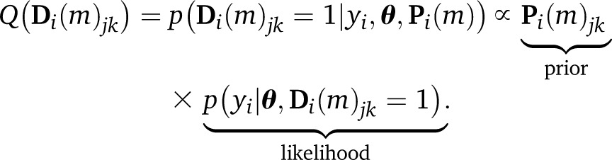(10)

This updating of diplotype state for each individual i = 1, … , n in light of phenotypic information reflects the following intuition: Suppose that prior to observing y, diplotype probabilities P₁, … , P_n−1 are well informed but P_n is not; if analysis with y reveals a clear pattern of effects (e.g., high phenotype values associated with particular diplotype states), then y_n provides information to update P_n. Moreover, it implies that different phenotypes could in theory promote different underlying diplotype states Δ—a useful feature when locus m is defined broadly enough to contain multiple recombinants and therefore multiple configurations of Δ, of which only one is relevant to the interrogated QTL.

The likelihood conditional on diplotype states, p(y|θ, Δ), is specified in terms of a GLMM with linear predictor

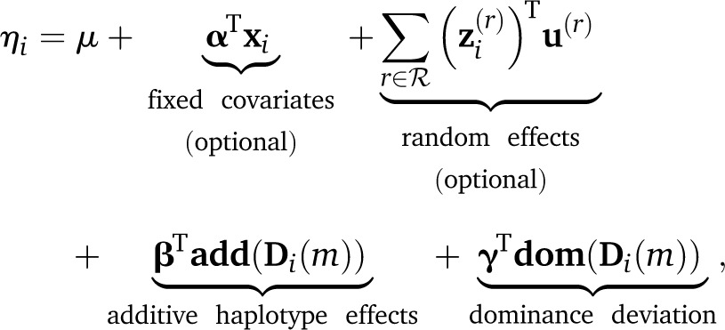(11)

where terms are included above for fixed effects α based on covariates in x_i and for an arbitrary set of variance components ℛ, each with incidence vector $z_i^{\left(r\right)}$ and effect vector modeled as $u^{\left(r\right)}\sim \text{N}\left(\mathbf{0},R^{\left(r\right)}{\tau }_r^2\right).$ Such additional terms are here defined loosely because our model is deliberately presented within established, extensible software that allows bespoke specification. In the current study, we demonstrate use of the following variance components: cage, where for c cages, R^(cage) = I_c; sibship, where for s sibships, R^(sibship) = I_s; and polygenic effects approximated by an animal model (hereafter, a “kinship” effect), where R^(kinship) = K is the s × s additive relationship matrix estimated from the pedigree (Kennedy et al. 1992). Haplotype effects β and dominance deviations γ are modeled hierarchically as $\beta \sim \text{N}\left(0,I{\tau }_{\text{add}}^2\right)$ and $\gamma \sim \text{N}\left(0,I{\tau }_{\text{dom}}^2\right)$; this hierarchical modeling benefits estimation in two ways—it allows information to be borrowed across effects on related scales, and it provides robustness to data sets where the sampling of diplotypes is sparse. The remaining parameters are given weak, conjugate priors: Fixed effects (μ, α) are given independent normal priors N(0, c), where c is large relative to the phenotype scale [e.g., c = 1000 for Var(y) = 1]; and dispersions σ², ${\tau }_{\text{add}}^2,$ ${\tau }_{\text{dom}}^2,$ and each ${\tau }_r^2$ are given inverse-gamma priors as in, e.g., Lenarcic et al. (2012). The complete Diploffect model, shown with a polygenic effect, is summarized using plate notation in Figure 1.

Figure 1.

The Diploffect model depicted as a directed acyclic graph. Dashed arrows indicate deterministic relationships and solid arrows indicate stochastic relationships. Shaded nodes are observed variables, and open nodes are unobserved variables, with a double circle representing the remaining parameters; priors are omitted. The number of instances of each variable is shown using plate notation.

The posterior of effects integrated in Equation 7 involves integrating over a J²ⁿ-dimensional space. We consider two alternatives for sampling from this posterior below.

Diploffect estimation by MCMC: DF.MCMC

Posteriors for all parameters in the Diploffect model can be estimated by Markov chain Monte Carlo (MCMC) by iterating two basic Gibbs sampling steps. At each iteration, k = 1, … , K:

• 1.
  Sample all effect variables θ^(k+1) given the previous iteration’s diplotypes Δ^(k),

  $${\mathit{\theta }}^{\left(k+1\right)}\sim p\left(\mathit{\theta }|y,{\Delta }^{\left(k\right)}\right).$$ (12)
• 2.
  Sample diplotypes Δ^(k+1) given effect variables θ^(k+1),

  $${\Delta }^{\left(k+1\right)}\sim p\left({\Delta }^{\left(k+1\right)}|\Psi ,{\mathit{\theta }}^{\left(k+1\right)},y\right).$$ (13)

Initial values for k = 1 are randomly sampled from their priors.

Although relatively efficient Gibbs sampling schemes for step 1 are well established (we use those provided in Plummer 2003; see Implementation details), step 2 requires special consideration. A straightforward approach is to sample from the full conditional, evaluating all diplotypes’ posterior probabilities in D_i(m) by Equation 10 and drawing a diplotype state for each individual in turn. Per individual, however, this incurs O(J²) computational time because it requires evaluating the function Q for all diplotypes. For the sake of efficiency, we develop an optimization, discrete slice sampling with prior reordering, described in Appendix A, which makes this sampling more efficient. Hereafter we refer to this method as Diploffect estimation by MCMC (DF.MCMC).

Diploffect estimation by importance sampling: DF.IS and DF.IS.kinship

Seeking a noniterative estimation procedure that is more efficient for standard GLMMs, we also provide a strategy based on Importance Sampling (IS) of integrated nested Laplace approximations (INLA). INLA provides a deterministic estimate of the multivariate posterior distribution of a GLMM (Rue et al. 2009), giving analytic approximations for effects and sampling approximations for variances. In our IS procedure, these posteriors are estimated conditional on diplotype for many possible diplotype configurations; they are then combined through reweighting to give a final mixture distribution that resembles more closely the integration of the full posterior in Equation 7. Specifically, the procedure is

• 1.Sample diplotypes Δ^(k) from their prior, Δ^(k) ∼ p(Ψ).
• 2.Obtain an INLA estimate of posterior p(θ|y, Δ^(k)) for effect variables θ^(k).
• 3.Obtain an INLA estimate of the marginal likelihood w^(k) = p(y|Δ^(k)).
• 4.Repeat steps 1–3 K times.
• 5.
  Estimate the posterior of any statistic of interest T(θ), using the weighted mixture

  $${\widehat{T}}_{\text{IS}}\left(\mathit{\theta }\right)=\frac{{\displaystyle {\sum }_{k}T\left({\mathit{\theta }}^{\left(k\right)}\right)w^{\left(k\right)}}}{{\displaystyle {\sum }_k{w}^{\left(k\right)}}},$$ (14)

  • where for each k, statistic T(θ^(k)) is calculated from the corresponding posterior p(θ|y, Δ^(k)) calculated in step 2.

Calculation of the weighting function w⁽¹⁾, … , w^(K) uses the marginal likelihood obtained from INLA and is described more fully in Appendix B. The statistic T(θ) is defined in this study according to the following requirements: for point estimation is needed, we use the posterior mean T(θ) = E(θ|y, Δ); for obtaining highest posterior density (HPD) intervals of effects parameters, T(θ) records the analytic approximation of p(θ|y, Δ); and for estimating the additive vs. dominance proportion, p(π_add|y), where ${\pi }_{\text{add}}={\tau }_{\text{add}}^2/\left({\tau }_{\text{add}}^2+{\tau }_{\text{dom}}^2\right),$ T(θ) records 1000 posterior samples from p(π_add|y, Δ).

Importance sampling of the above mixture model can be highly inefficient and lead to unstable results when the mixture prior p(Φ) is uninformed; in particular, a large number of samples drawn from the prior may, after reweighting, translate into a comparatively tiny number of samples from the posterior (Carlin and Louis 2008). To track sampling efficiency, we therefore use the effective sample size (ESS) metric of Liu et al. (2001) equivalent to $\text{ESS}={\left[{\displaystyle {\sum }_k{w}^{\left(k\right)}}\right]}^2/\left[{\displaystyle {\sum }_k{\left(w^{\left(k\right)}\right)}^2}\right]$ (Robert and Casella 2009).

Application of the IS procedure is denoted Diploffect estimation by importance sampling (DF.IS) in all cases except when the GLMM includes a kinship effect, in which case it is denoted DF.IS.kinship. This distinction is made in light of the fact that fitting kinship effects (as opposed to approximating them with, e.g., sibship effects) can incur significant additional computation.

Partial Bayesian approximation: DF.MCMC.pseudo and DF.IS.noweight

In cases where it can be assumed that p(Δ|Ψ) ≈ p(Δ|Ψ, y), for example, where the QTL effect is weak or the posteriors of the diplotypes are consistently vague across individuals, integration of the joint posterior in Equation 7 can be approximated as

$$p\left(\mathit{\theta }|\Psi ,y\right)\approx {\displaystyle \int p\left(\mathit{\theta }|\Delta ,\Psi ,y\right)\hspace{0.17em}p\left(\Delta |\Psi \right)\text{d}\Delta }.$$ (15)

This approximation, essentially a form of unweighted multiple imputation, is used by Durrant and Mott (2010) to estimate haplotype effects at QTL in populations of recombinant inbreds. By restricting attention to normally distributed traits with no covariates or structure, they develop a method to sample from the above pseudoposterior directly. To explore the utility of this approximation, we implement versions of it based on both DF.MCMC and DF.IS. In DF.MCMC.pseudo, the sampling of the posterior of Δ conditional on the current value of θ in Equation 13 is replaced by a draw from the prior, Δ^(k) ∼ p(Ψ); this method was recently used by us in the analysis of immune phenotypes in the pre-CC (Phillippi et al. 2014). In DF.IS.noweight, DF.IS is modified so that weights are uniform, i.e., w^(k) = 1 for all k; this approach is similar to that used in the Arabidopsis study of Kover et al. (2009), who instead estimate β via a fixed-effects regression.

Non-Bayesian approximations using regression on probabilities: partial.lm, ridge.add, and ridge.dom

ROP methods model the phenotype in a regression where diplotype states (and functions thereof) are represented by their corresponding probabilities of being present. Use of probabilities in this way, substituting functions of D_i(m) with functions of P_i(m), can provide stable estimation when P_i(m) probabilities are well informed; otherwise, when uncertainty is present, the design matrix can become multicollinear, making some effects nonidentifiable and thus ineligible for a fair comparison with the truth. Rather than providing a comprehensive survey of ROP, we therefore consider three illustrative examples that at least guarantee identifiability under all possible levels of haplotype uncertainty: a marginal estimator, partial.lm; and two ridge regression estimators, ridge.add and ridge.dom.

The marginal estimator partial.lm uses a single predictor linear model to estimate, for each founder haplotype in turn, the effect of that haplotype’s dosage on the phenotype; i.e.,

$${\eta }_i={\mu }_j+{\beta }_j{\left\{add\left(P_i\left(m\right)\right)\right\}}_j,$$

where β_j is the jth element of β. This method was used to estimate effects in the pre-CC study of Aylor et al. (2011).

In ridge.add, ridge regression (Hoerl and Kennard 1970) is applied to a ROP form of the additive model of Equation 1,

$${\eta }_i=\mu +{\beta }^{\mathsf{T}}add\left(P_i\left(m\right)\right),$$ (16)

with β estimated by minimizing ${\displaystyle {\sum }_i{\left(y_i-{\eta }_i\right)}^2+\lambda {\beta }^{\mathsf{T}}\beta },$ where tuning parameter λ is set by 10-fold cross-validation. In ridge.dom, an analogous model is fitted based on the additive plus dominance model of Equation 2,

$${\eta }_i=\mu +{\beta }^{\mathsf{T}}add\left(P_i\left(m\right)\right)+{\gamma }^{\mathsf{T}}dom\left(P_i\left(m\right)\right).$$ (17)

Implementation details

MCMC-based approaches (DF.MCMC and DF.MCMC.pseudo) were implemented in R (R Development Core Team 2011), JAGS (Plummer 2003), and rjags (Plummer 2014). JAGS is an open-source general MCMC sampling package; we implemented add-on code to support the partially Bayesian prior sampling of DF.MCMC.pseudo (see code in File S4). MCMC was performed for 5000 time steps, of which the first 1000 were discarded as burn-in, and the remaining 4000 were thinned at 1/10 to give 400 usable samples. Importance sampling approaches (DF.IS, DF.IS.noweight, and DF.IS.kinship) were implemented using the R package INLA (Rue et al. 2009). In each application of the IS methods we used 1000 independent samples directly drawn from the haplotype probabilities inferred by HAPPY (Mott et al. 2000; Mott 2009). Estimation of the additive relationship matrix was performed using the R package pedigreemm (Vazquez et al. 2010). Ridge regression was performed using the R package GLMNet (Friedman et al. 2010), with tuning parameters selected by 10-fold cross-validation. All other analysis was performed in R.

Data and Simulations

We use simulation to evaluate the ability of our Diploffect model to estimate haplotype and diplotype effects at a single QTL segregating in a multiparent population. It is assumed that the QTL location has been determined already and phenotype information per individual is available, but diplotype state at the QTL for each individual is available only as inferred diplotype probabilities. For methods in Table 2, we assess subsequent estimation in terms of both numerical accuracy and ability to rank effects under a range of QTL effect sizes and in different genetic contexts. Practical use of the Diploffect model is then illustrated through application to real, previously mapped QTL. Both simulation and application use data from two real populations: the incipient strains of the Collaborative Cross (pre-CC) (Aylor et al. 2011) and the Northport HS mice (Valdar et al. 2006a). These data sets are described below.

Pre-CC data set

The Collaborative Cross (Collaborative Cross Consortium 2012) is a large panel of recombinant inbred lines bred from a set of eight inbred founder mouse strains (abbreviated names in parentheses): 129S1/SvlmJ (129S1), A/J (AJ), C57BL/6J (B6), NOD/ShiLtJ (NOD), NZO/HILtJ (NZO), CAST/EiJ (CAST), PWK/PhJ (PWK), and WSB/EiJ (WSB). Breeding of the CC is an ongoing effort, and at the time of this writing a relatively small number of finalized lines are available. Nonetheless, partially inbred lines taken from an early stage of the CC breeding process, the so-called pre-CC population, have been studied and used for QTL identification (Aylor et al. 2011; Kelada et al. 2012; Ferris et al. 2013; Phillippi et al. 2014). The pre-CC data set analyzed here is that from the study of Aylor et al. (2011). This comprises data for 184 mice from 184 independent pre-CC lines (i.e., one replicate per line); these lines had attained on average 6.7 generations of inbreeding following the initial eight-way cross and as a result have genomes with ∼16% residual heterozygosity. Aylor et al. (2011) used HAPPY (Mott et al. 2000) to generate diplotype probability matrices for all 184 mice based on genotype information for 16,159 markers across the genome. For simulation purposes, we use the originally analyzed probability matrices for a subset of 50 loci spaced approximately evenly throughout the genome (provided in Supporting Information, File S1, and File S2). For data analysis, we consider the white head-spotting phenotype mapped by Aylor et al. (2011) to a QTL with a peak at 95.0 Mb on chromosome 10. This QTL data set comprises a binary phenotype value (presence or absence of a white head spot) defined for 110 nonalbino mice and diplotype probability matrices for the QTL peak.

HS data set

The heterogeneous stocks are an outbred population of mice also derived from eight inbred strains: AJ, AKR/J (AKR), BALBc/J (BALB), CBA/J (CBA), C3H/HeJ (C3H), B6, DBA/2J (DBA), and LP/J (LP). We used data from the study of Valdar et al. (2006a), which includes mice from approximately generation 50 of the cross and comprises genotypes and phenotypes for 1762 mice from 180 families, with family sizes varying from 8 to 48. Valdar et al. (2006a) also used HAPPY to generate diplotype probability matrices based on 10,148 markers across the genome. For simulation purposes, we use the originally analyzed probability matrices for a subset of 50 loci spaced approximately evenly throughout the genome (provided in File S1). For data analysis, we consider two phenotypes: total cholesterol (CHOL: 1656 observations), mapped by Valdar et al. (2006a) to a QTL at 171.5–172.0 Mb on chromosome 1; and the total startle time to a loud noise [fear potentiated startle (FPS): 1508 observations], which was mapped to a QTL at 91.37–92.62 Mb on chromosome 15. In each case, we use the original probability matrices defined at the peak loci; partial pedigree information; per-individual values for phenotype; and per-individual values for pre-determined covariates (defined in Valdar et al. 2006b)—sibship, cage, sex, testing chamber (FPS only), and date of birth (CHOL only) (all provided in File S3).

Simulating QTL effects

The ability of the Diploffect-based methods to estimate and rank haplotype and diplotype effects is assessed by simulation: We apply those methods, and their competitors listed in Table 2, to simulated single QTL for which the true effects are known. This is performed first using pre-CC data, which emphasizes estimation of haplotype (i.e., additive) effects, potentially in the presence of dominance from residual heterozygotes, and then separately using the HS data, which emphasizes estimation of diplotype effects that could arise from both additive and dominance genetics. In either population, simulation of QTL involves four basic steps: selecting a locus; assigning true diplotypes; assigning QTL effects; and simulating a phenotype based on the QTL effect, polygenic factors, and noise. This is described in detail below.

Let ℬ be a set of 50 representative haplotype effects (listed in File S1): 25 of these are binary alleles distributed among the eight founders [e.g., (0, 0, 0, 0, 1, 1, 1, 1), (0, 1, 1, 1, 1, 1, 1, 1)]; the remaining 25 were drawn from N(0, I₈). Let $\mathcal{V}=\left\{2.5,5,10,20,30,40\right\}$ be the set of percentages of variance explained considered to be attributable to the QTL effect. Simulations are performed in the following (factorial) manner: For each data set (pre-CC or HS), for each locus m from the 50 defined in that data set, for $\beta \in \mathbf{ℬ},$ and for dominance effects being either included or excluded, we perform the following simulation trial for every QTL effect size $v\in \mathcal{V}:$

• 1.For each individual i ∈ {1, … , n}, assign a true diplotype state by sampling D_i(m) ∼ p(P_i(m)).
• 2.If including dominance effects, draw γ ∼ N(0, I); otherwise, set γ = 0.
• 3.Calculate QTL contribution for each individual i as q_i = β^Τadd(D_i(m) + γ^Τdom(D_i(m)).
• 4.If HS, draw polygenic effect as n-vector u ∼ N(0, K_IBS) (see below); otherwise, if pre-CC, set u = 0.
• 5.Draw individual-specific noise as n-vector ε ∼ N(0, I_n).
• 6.Calculate the phenotype for each individual i as y_i = aq_i + bu_i + cε_i, where a, b, and c are constants used to adjust relative contributions of each term to the total phenotypic variance, ensuring that the QTL accounts for v%, polygenic effects account for 50% (in HS) or 0% (in pre-CC), and the remainder is attributed to individual-specific noise.
• 7.Assess the ability of each method to estimate QTL effects given only y and P₁(m), … , P_n(m).

In step 4, K_IBS is the realized genomic relationship matrix calculated using EMMA (Kang et al. 2008), applied to the entire set of HS genotypes. This polygenic effect, which represents potentially confounding effects of other QTL, is simulated only for the HS; the pre-CC lines are (in expectation) genetically exchangeable, and it is therefore assumed (for simulation purposes) that polygenic effects in the pre-CC would be indistinguishable from individual-specific noise. Also, because of this, in the pre-CC simulations we do not evaluate method DF.IS.kinship.

The above simulation scheme describes 2 × 50 × 50 × 6 × 2 = 60 × 10³ distinct experimental conditions; this makes evaluating some methods in some populations impractical—specifically, DF.MCMC and DF.MCMC.pseudo are not evaluated in simulations involving the HS.

Evaluating estimation of QTL effects

Methods are evaluated based on their accuracy in determining two types of information: (1) the relative shift in phenotype value associated with a given diplotype substitution, which we measure across all such substitutions using an adjusted mean square error (the “effect MSE”), and (2) the relative ordering of the diplotype effect series, which we measure by agreement of ranks (the “effect rank accuracy”). Both types of information we consider highly relevant to subsequent experimental and/or bioinformatic characterization of QTL detected in multiparent populations.

Effect MSE and effect rank accuracy are defined as follows. Let θ denote the p-vector of simulated effects (the target) after mean centering, and let $\widehat{\theta }$ be the p-vector of point estimates for the target, also after mean centering. Note that mean centering is performed both to adjust for the fact that the estimation models are naturally overspecified (e.g., the intercepts are redundant) and to reflect the fact that scientific interest is more meaningfully focused on substitution effects relative to each other (both in magnitude and in rank) than in absolute terms. The estimator $\widehat{\theta }$ is defined according to the method used: For Bayesian or partially Bayesian methods in Table 2 (DF.IS, DF.IS.kinship, DF.IS.noweight, DF.MCMC, and DF.MCMC.pseudo) it is defined as the posterior mean; for the remaining methods (partial.lm, ridge.add, and ridge.dom) it is the standard point estimate (i.e., that maximizing the likelihood or penalized likelihood). The effect MSE is then defined as the average squared difference between parameters in target and estimate, normalized by the variance of the target; i.e.,

$$\text{Effect}\hspace{0.5em}\text{MSE}=\frac{{\left(\widehat{\theta }-\mathit{\theta }\right)}^{\mathsf{T}}\left(\widehat{\theta }-\mathit{\theta }\right)}{p\times \text{Var}\left(\mathit{\theta }\right)}.$$ (18)

The effect rank accuracy is measured by Spearman’s rank correlation of θ and $\widehat{\theta }.$

The set of effects included in the target θ differs according to the population. For the pre-CC, which is almost inbred, the target includes only the haplotype (additive) effects, i.e., θ = β; dominance effects may be present, but the infrequency of heterozygotes in the pre-CC precludes their meaningful estimation, making them akin to a type of confounding noise in the pre-CC. For the HS, many heterozygous diplotype states will be present at a given QTL, although overall some diplotype states may be absent; the target is therefore the J × (J + 1)/2 vector of diplotype effects; i.e., θ = δ.

Evaluating improvement in diplotype inference

Application of the Diploffect model leads not only to posteriors for QTL effects but also to updated probabilities for each individual’s diplotype state (see Statistical Models and Methods, Equation 8, and Figure A1); because the simulations described above actually generate diplotype states for each individual (step 1), in postsimulation analysis it is possible to observe to what extent these updated probabilities are closer to the truth. We quantify this using a summary statistic, the true diplotype improvement (TDI). Letting jk[i] index the true diplotype for individual i, such that {D_i(m)}_jk[i] ≡ D_i(m)_jk[i] = 1, the TDI measures, over all true diplotypes, the average increase in probability from prior to posterior, i.e.,

$$\text{TDI}=\frac{1}{n}{\displaystyle \sum _{i=1}^n\left[p\left(D_i{\left(m\right)}_{jk\left[i\right]}|\Psi ,y\right)-P_i{\left(m\right)}_{jk\left[i\right]}\right]}.$$ (19)

Results

Pre-CC simulations

Methods were evaluated on their ability to estimate additive (haplotype) effects at simulated QTL in the pre-CC. Figure 2 shows performance when the QTL effect simulated was entirely additive; Figure 3 shows performance when the simulated effect also included dominance. In the latter case, dominance was not the target of inference as such—the mostly inbred pre-CC can manifest dominance only through residual heterozygosity; rather, it was included as a form of noise, potentially disrupting additive effect estimation. Comparison of Figure 2 and Figure 3 reveals this disruptive effect to be slight (at least for dominance effects simulated here), causing an overall increase in effect MSE and a decrease in effect rank accuracy; otherwise there were few qualitative differences in relative performance across methods.

Figure 2.

(A and B) Estimation of additive effects for a simulated additive-acting QTL in the pre-CC population, judged by (A) prediction error and (B) rank accuracy. For a given combination of QTL effect size and estimation method, each point indicates the mean of the evaluation metric based on 2500 simulation trials, and each vertical line indicates the 95% confidence interval of that mean. Points and lines are grouped by the corresponding QTL effect sizes and also are shifted slightly to avoid overlap. At the same QTL effect size, left to right jittering of the methods reflects relative performance from better to worse.

Figure 3.

(A and B) Estimation of additive effects for a QTL simulated to have both additive and dominant effects in the pre-CC population. Symbols are defined as in Figure 2.

For both types of QTL effect, strong performance was seen across all effect sizes and metrics by implementations of Diploffect DF.MCMC (best) and DF.IS and ridge estimator ridge.add. Other methods produced competitive performance only in some settings and by some criteria. In particular, although the MSE of ridge.dom was worse than that of most other methods, and the MSE of partial.lm was worst of all (especially for QTL effect sizes <10%), both achieved competitive rank accuracy; this suggests that under this setting, and relative to a full probabilistic model, these ROP methods give estimates that are inflated (and therefore strongly penalized by MSE) but not necessarily poorly ordered.

Comparison of Bayesian methods DF.MCMC and DF.IS with their partially Bayesian approximations DF.MCMC.pseudo and DF.IS.noweight reflected some advantages of the Bayesian methods. DF.IS outperformed its approximation DF.IS.noweight in terms of MSE when the QTL effect was strong and matched it when the QTL effect was weak; similarly, DF.MCMC consistently outperformed approximation DF.MCMC.pseudo in rank accuracy for all QTL effect sizes. Both these observations can be explained in part by the fact that the Diploffect model when implemented fully makes more efficient use of phenotype data—not only using those data to inform the QTL effects, but also then using those QTL effects to help resolve uncertainty in diplotype state. This phenomenon is reflected in Figure 4, which uses results from DF.MCMC to demonstrate that as the strength of the QTL is increased, the posterior distribution of diplotype state at the QTL is moved consistently closer to the truth.

Figure 4.

Increased posterior probability placed on the true diplotype at QTL simulated in the pre-CC, as analyzed using DF.MCMC.

Heterogeneous Stock simulations

The HS population represents a far more challenging target for inference of QTL effects than the pre-CC largely because its haplotype composition, inferred from a smaller number of genotyped markers on a more highly recombinant genome, is far more uncertain. This increased uncertainty is illustrated in Figure 5, which plots the distribution of the scaled selective information content (SIC) (a rescaling of the negated Shannon entropy, previously used for this purpose in, e.g., Rönnegård and Valdar 2011). Although locus information varies in both populations, and the pre-CC manifests uncertainty for some individuals even at those loci that are overall most informed, the HS has many individuals whose diplotype state is almost uninformed.

Figure 5.

Certainty of inferred diplotype assignments across all marker loci in the pre-CC and HS.

Methods were evaluated on their ability to estimate simultaneously 36 diplotype effects for QTL simulated in the HS, with separate simulation studies for QTL with effects of additive vs. effects of additive plus dominance. Excluded from these simulations were the MCMC methods, owing to their impractically slow mixing: The time required for acceptable MCMC convergence on this relatively large data set (1762 individuals) made performing 5000 trials at each QTL effect size unfeasible (see Table 3 and Data and Simulations section). The Diploffect model was therefore represented by importance samplers DF.IS, DF.IS.noweight, and DF.IS.kinship. Of these, genetic background effects arising from unequal relatedness were represented in two ways: DF.IS.kinship, which used a pedigree-derived animal model; and DF.IS and DF.IS.noweight, which used instead a simple random intercept for sibship—an approximation that reduced their running time by more than fourfold (Table 3). We note that the polygenic effect used to generate the simulated phenotypes corresponded to neither of these estimation models, but was instead based on realized genomic relationships in the HS (see Data and Simulations).

Table 3. Running time in seconds of different methods applied to simulated QTL in the pre-CC and HS data sets.

Population	Pre-CC	Heterogeneous stock
partial.lm	0.056	2.72
ridge.add	0.124	2.80
ridge.dom	0.151	2.92
DF.MCMC.pseudo	27.96	NA
DF.MCMC	92.77	NA
DF.IS.noweight	580.7	3,727
DF.IS	580.9	3,724
DF.IS.kinship	NA	16,231

As shown in Figure 6 and Figure 7, methods based on the Diploffect model strongly outperformed ROP-based competitors. This is somewhat expected: In the face of uncertainty, ROP will lead to often highly inflated estimates and resulting poor MSE (see discussion of Table 1 in Statistical Models and Methods). In this context, ridge regression should improve considerably over standard least-squares multivariable regression. Nonetheless, ridge.add produced effect estimates that were considerably dispersed relative to their true values, and ridge.dom performed so poorly (prediction error >2000 for 2.5%; see File S1) that it had to be excluded from Figure 6A and Figure 7A for legibility.

Figure 6.

(A and B) Estimation of diplotype effects for an additive-only QTL simulated in the HS. Symbols are defined as in Figure 2.

Figure 7.

(A and B) Estimation of diplotype effects for QTL simulated to have both additive and dominance effects in the HS. Symbols are defined as in Figure 2.

The addition of dominance effects to the simulated QTL reduced rank accuracy among all methods (Figure 8B) but did not alter relative performance. The plots showing MSE in the HS for different types of QTL effect (i.e., Figure 6A and Figure 8A) are not directly comparable in scale because of the way in which this metric is normalized (i.e., the denominator in Equation 18 is greater owing to greater variance of the target estimand); nonetheless, the pattern of performance among methods changes little between the additive setting and additive plus dominance—this is perhaps most surprising for ridge.dom, whose performance benefits so little from its additional dominance parameterization.

Figure 8.

Density plot of the effective sample size (ESS) of posterior samples for the DF.IS method (maximum possible is 1000) applied to HS and pre-CC when analyzing a 10% QTL with additive and dominance effects. The plot shows that ESS is more efficient in the pre-CC data set than in the HS, reflecting the much larger dimension of the posterior in modeling QTL for the larger and less informed HS population.

For QTL effect sizes of ≥10%, MSE was controlled best by Diploffect models DF.IS and DF.IS.kinship; for smaller effect QTL, however, the less informed, partially Bayesian method DF.IS.noweight was seen to retain its accuracy while that of the more fully Bayesian models deteriorated. As with the pre-CC simulations above, this may reflect a trade-off between modeling sophistication and computational stability: DF.IS allows phenotype to inform descent, but to do so it must reweight each of its 1000 prior samples using an importance function, which, when the posterior is far from the prior, can drastically reduce sampling efficiency, leading to erratic results when sampling is capped, as in these simulations; DF.IS.noweight does not allow phenotype to inform descent but also does not require its samples to be reweighted, leading to pseudo-posteriors that are nonetheless well estimated. The need for using many more importance samples when applying DF.IS to the HS rather than to the pre-CC is illustrated in Figure 8, which shows for DF.IS analysis of 10% QTL the distribution of the effective sample size (ESS) statistic (see Statistical Models and Methods).

Finally, we note that in estimating both types of QTL effects, modeling genetic background using a kinship-specified polygenic effect, as in DF.IS.kinship, was not clearly superior to using a sibship-based approximation—indeed, at least in this context, it performed worse on rank accuracy while requiring substantially more computation. We speculate that this relative robustness of the sibship approximation could reflect either the circular-mated breeding scheme of the HS leading to kinship being well approximated by sibship, or/and computational efficiencies associated with estimating random effects with more complex covariance structures (which may lead to, for example, smaller ESS values), rather than any advantage of sibship approximations in general.

Haplotype effects on a binary outcome: white head spotting in the pre-CC

The pre-CC study of Aylor et al. (2011) identified a Mendelian trait locus on chromosome 10 (at 92.0 Mb) for white head spotting. White head spotting is a characteristic of the inbred CC founder strain WSB, and this phenotype was visibly present in 6 of the 110 nonalbino pre-CC mice. Because the identified locus was dominant Mendelian, associated with the presence of either one or two WSB haplotypes, it was straightforward to identify by LD mapping using a ROP model as in Equation 16. Estimating meaningful strain effects was not, in this case, necessary, because the effect was obvious. Such estimation would, however, have been awkward statistically because proper treatment of the binary outcome is most naturally modeled as a binary logistic regression, which in a standard maximum-likelihood estimation would have quickly become problematic due to separation (see, e.g., Gelman and Hill 2007). We considered estimation using Diploffect, which, as a GLMM with hierarchical shrinkage on the strain effects, models the white spot data without further development. Figure 9 plots 95% highest posterior density (HPD) intervals for all haplotype effects at the QTL estimated by both DF.MCMC and DF.IS. Both models report a similar result for this QTL: The non-WSB posteriors are similar to each other and broad, reflecting high uncertainty about the relative effects of these strains; the WSB posterior distribution is shifted above the others, reflecting its positive effect. The HPD of the contrast WSB vs. the other strains, calculated by applying this contrast to each MCMC sample from DF.MCMC, is 1.35–36.18, further reflecting the positive effect of the WSB haplotype but also the fact that uncertainty about this effect remains because the sample size is not infinite.

Figure 9.

Highest posterior density intervals (95%, 50% and mean) for the haplotype effects of the binary trait white spotting in the pre-CC.

Haplotype and diplotype effects at QTL in the HS: FPS and CHOL

To demonstrate Diploffect-based estimation of additive and dominance effects, we examined two previously detected QTL from the HS mapping study of Valdar et al. (2006a). The first QTL examined was for fear potentiated startle (a conditioned test of anxiety), located between 91.37 and 92.62 Mb on chromosome 15. To the central marker interval of the FPS QTL (rs3722990–rs3716673), we fitted a Diploffect linear mixed model (LMM) using DF.IS that included fixed effects of sex and testing chamber and random effects of cage and sibship, and where FPS was subject to a cube root transformation; this model specification follows that described in the parallel HS study of Valdar et al. (2006b). The results of the DF.IS analysis are shown in Figure 10 and Figure 11. Figure 10A shows HPD intervals for the haplotype effects. Dominance effects, which comprise 28 deviations from the additive haplotype model, are harder to graph intuitively; instead we plot the posterior predictive means of the 36 possible diplotype effects, i.e., E(δ|y), as a symmetric grayscale matrix in Figure 10B. Both plots suggest that effects are driven by C57BL/6J, and the consistent banding pattern of the diplotype effect plot suggests these effects are mainly additive. Figure 11 more directly quantifies the extent to which the QTL effects are additive vs. dominant: It plots the posterior of the proportion of hyperparameter variance attributable to additive effects (see Statistical Models and Methods). The mode of this distribution is close to 1 but, as expected for a quantity defined using hyperparameters, the distribution itself is very broad (posterior mean 0.546), reflecting a high degree of uncertainty.

Figure 10.

(A and B) Haplotype (A) and diplotype (B) effects estimated by DF.IS for phenotype FPS in the HS.

Figure 11.

Posteriors of the fraction of effect variance due to additive rather than dominance effects at QTL for phenotypes FPS and CHOL in the HS data set.

The second QTL examined in the HS was for total cholesterol concentration, located between 171.15 and 171.51 Mb on chromosome 1. To the central marker interval of the CHOL QTL (rs13476229–rs3657320), we fitted a Diploffect LMM using DF.IS that included fixed effects of sex and birth month, and random intercepts for cage and sibship (again following Valdar et al. 2006b). Results of this analysis are shown in Figure 11 and Figure 12. Unlike the FPS QTL, the HPD intervals for CHOL (Figure 12A) cluster into three different groups: the highest effect from LP, a second group comprising C3H and CBA with positive mean effects, and the remaining five strains having negative effects. This pattern is consistent with a multiallelic QTL, potentially arising through multiple, locally epistatic biallelic variants. In the diplotype effect plot (Figure 12B), although most of the effects are additive, off-diagonal patches provide some evidence of dominance effects—in particular, the haplotype combinations AKR × DBA and C3H × CBA deviate from the banding otherwise expected under additive genetics. The fraction of additive QTL effect variance for CHOL in Figure 11 is, however, strongly skewed toward additivity (posterior mean 0.717, with a sharp peak near 1), suggesting that additive effects predominate.

Figure 12.

(A and B) Haplotype (A) and diplotype (B) effects estimated by DF.IS for phenotype CHOL in the HS.

Discussion

We present here a statistical model and associated computational techniques for estimating the marginal effects of alternating haplotype composition at QTL detected in multiparent populations. Our statistical model is intuitive in its construction, connecting phenotype to underlying diplotype state through a standard hierarchical regression model. Its chief novelty, and the source of greatest statistical challenge, is that diplotype state, although efficiently encapsulating multiple facets of local genetic variation, cannot be observed directly and is typically available only probabilistically—meaning that statistically coherent and predictively useful description of QTL action requires estimating effects of haplotype composition from data where composition is itself uncertain. We frame this problem as a Bayesian integration, in which both diplotype states and QTL effects are latent variables to be estimated, and provide two computational approaches to solving it: one based on MCMC, which provides great flexibility but is also heavily computationally demanding, and the other using importance sampling and noniterative Bayesian GLMM fits, which is less flexible but more computationally efficient. Importantly, in theory and simulation, we describe how simpler, approximate methods for estimating haplotype effects relate to our model and how the trade-offs they make can affect inference.

An important comparison is made between Diploffect and approaches based on Haley–Knott regression, which regress on the diplotype probabilities themselves (or functions of them, such as the haplotype dosage) rather than the latent states those probabilities represent. In the context of QTL detection, where the need to scan potentially large numbers of loci makes fast computation essential, we believe that such ROP-based approaches are typically well justified and often the only practical solution. But for estimating effects at detected QTL, where the number of loci interrogated will be fewer by several orders of magnitude and the amount of time and energy devoted to interpretation will be far greater, there is room for a different trade-off.

We do expect ROP to provide accurate effect estimates under some circumstances. When, for example, descent can be determined with near certainty (as may become more common as marker density is increased), a design matrix of diplotype probabilities (and haplotype dosages) will reduce to zeros and ones (and twos); in this case, although hierarchical modeling of effects would induce useful shrinkage, modeling diplotypes as latent variables would produce comparatively little benefit. This is demonstrated in the results of ridge regression (ridge.add) on the pre-CC: In this context, with only moderate uncertainty for most individuals at most loci, the performance of a simple ROP-based eight-allele ridge model (which we consider an optimistic equivalent to an unpenalized regression of the same model) approaches that of the best Diploffect-based method. Adding dominance effects to this ridge regression (which again we consider a more stable equivalent to doing so with an ordinary regression) produces effect estimates that are far more dispersed. Applying these stabilized ROP approaches to the HS data set, whose higher ratio of recombination density to genotype density implies a less certain haplotype composition, leads to effect estimates that can be erratic; indeed, such point estimates should not be taken at face value without substantial caveats or examining (if possible) likely estimator variance. In populations and studies where this ratio is lower, and haplotype reconstruction is more advanced (e.g., in the DO population of Svenson et al. 2012 and Gatti et al. 2014), or where the number of founders is small relative to the sample size, we expect that additive ROP models will often be adequate, if suboptimal. Only in extreme cases, however, do we expect that reliable estimation of additive plus dominance effects will not require some form of hierarchical shrinkage.

A strong motivation for developing Diploffect, and in particular to use a Bayesian approach to its estimation, is to facilitate design of follow-up studies—in particular, the ability to obtain for any future combination of haplotypes, covariates, and concisely specified genetic background effects a posterior predictive distribution for some function of the phenotype. This could be, for example, a cost or utility function whose posterior predictive distribution can inform decisions about how to prioritize subsequent experiments. Such predictive distributions are easily obtained from our MCMC procedure and can also be extracted with only slightly more effort [via specification of T(θ) in Equation 14] from our importance sampling methods. We anticipate that, applied to (potentially multiple) independent QTL, Diploffect models could provide more robust out-of-sample predictions of the phenotype value in, e.g., proposed crosses of multiparental recombinant inbred lines than would be possible using ROP-based models.

Use of the Bayesian procedures proposed here nonetheless has several potential drawbacks, foremost among which is computation time: Although our modified slice sampler (DF.MCMC; Appendix A) makes MCMC sampling of both diplotypes and effects feasible, it is highly computationally intensive. For large outbred populations, especially those with a high degree of diplotype uncertainty, we therefore prefer our importance sampler (DF.IS). For either method, however, a high degree of diplotype uncertainty and weak QTL effects result in computational inefficiency, since the posterior distribution that must be traversed (in MCMC) or sampled (in IS) is much more diffuse: For DF.MCMC this means convergence must be carefully monitored; for DF.IS, this means many more samples must be taken to achieve a reasonable picture of the posterior.

In light of the additional computational costs incurred by jointly modeling diplotypes and effects, it is worth considering the utility of partially Bayesian approaches in which diplotypes are multiply imputed, as in, for example, Kover et al. (2009) or Durrant and Mott (2010). Indeed, in discussing their partially Bayesian but highly computationally efficient random haplotype effects model, Durrant and Mott (2010) warn that Bayesian updating of the joint model described here would likely suffer from the label-switching problem (Stephens 1997). We consider this somewhat pessimistic: The label-switching problem usually occurs when the prior on the mixture components (in this case, the set of diplotype probabilities in Ψ) is uniform or nearly uniform; in practice, diplotype probabilities from modern haplotype reconstructions tend to be well informed enough for most individuals (even in the HS data set reported here) that label switching will be minimal, negligibly impact inference. Nonetheless, although our more fully Bayesian modeling adds value to inference when QTL effect sizes are large, when QTL effect sizes are small (≤10%), the partially Bayesian approximations DF.MCMC.pseudo and DF.IS.noweight become more competitive. Indeed, we observe that when analyzing small effect QTL (≤10%) in the high-dimensional/low-information setting of the HS data set, DF.IS.noweight outperformed its fully Bayesian counterpart, reflecting a potential trade-off between statistical and computational efficiency.

At greater computational cost, our modeling of QTL effects could be more comprehensive. At one extreme, we could consider a complete probabilistic treatment, for example in the spirit of Lin and Zeng (2006), whereby QTL effects and diplotypes are estimated conditional on raw genotype data, rather than, as here, conditional on diplotype probabilities that have been inferred previously and independently. Alternatively, and more realistically, we could attempt to model diplotype states explicitly at all contributing QTL, rather than, as here, focusing on marginal effects at a single QTL and presuming that all other effects can be can be well approximated by covariates and structured noise. Instead we provide a starting point—one that, while somewhat computationally demanding, relies on previously computed results (HMM output) and standard simplifying assumptions. In implementing Diploffect through an adaptation of existing, flexible modeling software (JAGS and INLA), we further aim that other researchers will be able to extend the model to better suit the specifics of a given phenotype, covariate structure, or experimental setting.

Appendix A

Discrete Slice Sampling with Reordering of Prior Probabilities

To help efficiently traverse the space of possible diplotype states during sampling of each D_i(m) in Equation 13, we propose an optimization of the discrete slice sampling algorithm of Neal (2003). First, we describe the original algorithm, which adapts slice sampling on a continuous density to the discrete case. Let T(jk) represent diplotype jk’s order in the range 1, … , J × (J + 1)/2, and define two boundary diplotypes for T(L) = 0 and T(R) = J × (J + 1)/2 + 1, with posterior probabilities for these set to zero. For the previous diplotype sampled, x′, first evaluate $S=Q\left(D_i{\left(m\right)}_{T^{-1}\left(x^{\prime }\right)}\right),$ and then sample an auxiliary variable q ∼ U(0, S). After that, expand a region [l, u] satisfying Q(l) ≥ q and Q(l − l) < q and Q(u) < q and Q(u) ≥ q. From the uniform distribution defined on [u, l], continue sampling the new diplotype status x^new until one is reached for which $Q\left(D_i{\left(m\right)}_{T^{-1}\left(x\right)}\right)\ge q.$ The diplotype posterior in Equation 10 is evaluated only a few times during each iteration, and thus it is much faster than full sampling.

Directly applying discrete slice sampling as above with the diplotype states ordered arbitrarily (e.g., alphabetically) will typically produce a prior and a posterior that are highly multimodal; this leads to extremely slow mixing, with posterior updates remaining stuck for many MCMC iterations within islands of higher-probability diplotypes separated by barrier-forming groups of lower-probability diplotypes (Figure A1A). To improve mixing, we introduce a small modification: Before applying slice sampling, we first reorder all J × (J + 1)/2 entries in matrix D_i(m) according to their prior probabilities in P_i(m). As shown in Figure A1B, this creates a prior that is monotone decreasing, removes the barrier, and results in posteriors that are more efficiently mixed (Figure A1C).

Figure A1.

Reordering of prior probabilities in the discrete slice sampler, using as an example the diplotype probabilities from haplotype reconstruction on the pre-CC. Diplotypes are represented by different letters, and 23 diplotypes with very low probabilities are omitted. The true diplotype, selected during simulation, is shaded black. An arbitrary ordering of diplotypes is shown in A and illustrates the problem to be addressed: If the initially sampled diplotype is M, the slice sampler cannot easily cross the barrier region to sample other high-probability diplotypes. Reordering the diplotypes by their prior probabilities to create a smoother distribution, as in B, removes this barrier region and allows the sampler to move easily between its initial value and all other values of high to moderate probability. C shows the posterior of this distribution given phenotype data (from the DF.MCMC procedure), in which the true diplotype’s posterior probability is increased.

Appendix B

Importance Sampling Using the Diplotype Prior and the Conditional Effects Posterior

Method DF.IS approximates statistics on the joint posterior p(Δ, β|y) by importance sampling. The IS procedure it uses owes its efficiency to INLA (Rue et al. 2009) and, in particular, to deterministic results for p(β|Δ, y) and p(y|Δ). This approach is explained in more detail here. Importance sampling, when used to estimate posterior statistics on disjoint parameter sets a and b whose joint posterior density p(a, b|y) is hard to sample from directly, describes the following general strategy: Sample a large number of times from a more tractable density g(a, b) (the importance function) and then reweight each sample relative to the others using importance weight w(a, b) = p(a, b|y)/g(a, b). In this article, a ≡ Δ, b ≡ β, with independent priors p(a, b) = p(a)p(b); additionally, due to INLA, deterministic approximations are available for both the conditional effects posterior p(b|y, a) and the conditional marginal likelihood p(y|a). Considered together, these features suggest an importance function g(a, b) = p(b|a, y)p(a), whereby each importance sample $\left(a_{\text{IS}}^{\left(k\right)},b_{\text{IS}}^{\left(k\right)}\right)$ for k = 1, … , K is generated by first sampling $a_{\text{IS}}^{\left(k\right)}$ from diplotype prior p(a) and then sampling $b_{\text{IS}}^{\left(k\right)}$ from conditional effects posterior $p\left(b|a_{\text{IS}}^{\left(k\right)},y\right).$ Since only the difference between sampling from g(a, b) and sampling from p(a, b|y) is the use of p(a) rather than p(a|y), the importance weight for each $\left(a_{\text{IS}}^{\left(k\right)},b_{\text{IS}}^{\left(k\right)}\right)$ pair is proportional only to $p\left(y|a_{\text{IS}}^{\left(k\right)}\right);$ that is,

$$\begin{array}{c}w\left(a,b\right)=\frac{p\left(a,b|y\right)}{g\left(a,b\right)}=\frac{p\left(a,b|y\right)}{p\left(b|y,a\right)p\left(a\right)}=\frac{p\left(a,b|y\right)}{\frac{p\left(a,b|y\right)p\left(a\right)}{p\left(a|y\right)}}\\ =\frac{p\left(a|y\right)}{p\left(a\right)}\times \frac{p\left(y\right)}{p\left(y\right)}=\frac{p\left(a,y\right)}{p\left(a\right)p\left(y\right)}=\frac{p\left(\mathbf{y}|a\right)}{p\left(y\right)}\propto p\left(\mathbf{y}|a\right).\end{array}$$

These proportionally defined weights can then be renormalized by their sum and used to appropriately reweight statistics on each sampled $\left(a_{\text{IS}}^{\left(k\right)},b_{\text{IS}}^{\left(k\right)}\right),$ as in Equation 14 (refer to Statistical Models and Methods).

Literature Cited

- Aylor D. L., Valdar W., Foulds-Mathes W., Buus R. J., Verdugo R. A., et al. , 2011. Genetic analysis of complex traits in the emerging Collaborative Cross. Genome Res. 21(8): 1213–1222 [DOI] [PMC free article] [PubMed] [Google Scholar]
- Bandillo N., Raghavan C., Muyco P. A., Sevilla M. A. L., Lobina I. T., et al. , 2013. Multi-parent advanced generation inter-cross (MAGIC) populations in rice: progress and potential for genetics research and breeding. Rice 6(1): 11. [DOI] [PMC free article] [PubMed] [Google Scholar]
- Baud A., Hermsen R., Guryev V., Stridh P., Graham D., et al. , 2013. Combined sequence-based and genetic mapping analysis of complex traits in outbred rats. Nat. Genet. 45(7): 767–775 [DOI] [PMC free article] [PubMed] [Google Scholar]
- Broman K. W., Sen S., 2009. A Guide to QTL Mapping with R/qtl. Springer-Verlag, New York [Google Scholar]
- Carlin B. P., Louis T. A., 2008. Bayesian Methods for Data Analysis, Ed. 3 Chapman & Hall/CRC, Boca Raton, FL [Google Scholar]
- Cavanagh C., Morell M., Mackay I., Powell W., 2008. From mutations to MAGIC: resources for gene discovery, validation and delivery in crop plants. Curr. Opin. Plant Biol. 11(2): 215–221 [DOI] [PubMed] [Google Scholar]
- Churchill G. A., Airey D. C., Allayee H., Angel J. M., Attie A. D., et al. , 2004. The Collaborative Cross, a community resource for the genetic analysis of complex traits. Nat. Genet. 36(11): 1133–1137 [DOI] [PubMed] [Google Scholar]
- Collaborative Cross Consortium , 2012. The genome architecture of the Collaborative Cross mouse genetic reference population. Genetics 190: 389–401 [DOI] [PMC free article] [PubMed] [Google Scholar]
- Durrant C., Mott R., 2010. Bayesian quantitative trait locus mapping using inferred haplotypes. Genetics 184: 839–852 [DOI] [PMC free article] [PubMed] [Google Scholar]
- Ferris M. T., Aylor D. L., Bottomly D., Whitmore A. C., Aicher L. D., et al. , 2013. Modeling host genetic regulation of influenza pathogenesis in the collaborative cross. PLoS Pathog. 9(2): e1003196. [DOI] [PMC free article] [PubMed] [Google Scholar]
- Friedman J., Hastie T., Tibshirani R., 2010. Regularization paths for generalized linear models via coordinate descent. J. Stat. Softw. 33(1): 1. [PMC free article] [PubMed] [Google Scholar]
- Gatti, D. M., K. L. Svenson, A. Shabalin, L. Wu, W. Valdar et al., 2014 Quantitative trait locus mapping methods for diversity outbred mice. G3 9: 1623–1633 [DOI] [PMC free article] [PubMed] [Google Scholar]
- Gelman A., Hill J., 2007. Data Analysis Using Regression and Multilevel/Hierarchical Models. Cambridge University Press, New York [Google Scholar]
- Haley C. S., Knott S. A., 1992. A simple regression method for mapping quantitative trait loci in line crosses using flanking markers. Heredity 69(4): 315–324 [DOI] [PubMed] [Google Scholar]
- Hoerl A. E., Kennard R. W., 1970. Ridge regression: biased estimation for nonorthogonal problems. Technometrics 12(1): 55–67 [Google Scholar]
- Huang B. E., George A. W., 2011. R/mpMap: a computational platform for the genetic analysis of multiparent recombinant inbred lines. Bioinformatics 27(5): 727–729 [DOI] [PubMed] [Google Scholar]
- Huang B. E., George A. W., Forrest K. L., Kilian A., Hayden M. J., et al. , 2012. A multiparent advanced generation inter-cross population for genetic analysis in wheat. Plant Biotechnol. J. 10(7): 826–839 [DOI] [PubMed] [Google Scholar]
- Huang G.-J., Shifman S., Valdar W., Johannesson M., Yalcin B., et al. , 2009. High resolution mapping of expression QTLs in heterogeneous stock mice in multiple tissues. Genome Res. 19(6): 1133–1140 [DOI] [PMC free article] [PubMed] [Google Scholar]
- Huang X., Paulo M.-J., Boer M., Effgen S., Keizer P., et al. , 2011. Analysis of natural allelic variation in Arabidopsis using a multiparent recombinant inbred line population. Proc. Natl. Acad. Sci. USA 108(11): 4488–4493 [DOI] [PMC free article] [PubMed] [Google Scholar]
- Johannesson M., Lopez-Aumatell R., Stridh P., Diez M., Tuncel J., et al. , 2009. A resource for the simultaneous high-resolution mapping of multiple quantitative trait loci in rats: the NIH heterogeneous stock. Genome Res. 19(1): 150–158 [DOI] [PMC free article] [PubMed] [Google Scholar]
- Kang H. M., Zaitlen N. A., Wade C. M., Kirby A., Heckerman D., et al. , 2008. Efficient control of population structure in model organism association mapping. Genetics 178: 1709–1723 [DOI] [PMC free article] [PubMed] [Google Scholar]
- Kelada S. N. P., Aylor D. L., Peck B. C. E., Ryan J. F., Tavarez U., et al. , 2012. Genetical analysis of hematological parameters in incipient lines of the Collaborative Cross. G3 2: 157–165 [DOI] [PMC free article] [PubMed] [Google Scholar]
- Kennedy B. W., Quinton M., van Arendonk J. A., 1992. Estimation of effects of single genes on quantitative traits. J. Anim. Sci. 70(7): 2000–2012 [DOI] [PubMed] [Google Scholar]
- King E. G., Merkes C. M., McNeil C. L., Hoofer S. R., Sen S., et al. , 2012a. Genetic dissection of a model complex trait using the Drosophila Synthetic Population Resource. Genome Res. 22: 1558–1566 [DOI] [PMC free article] [PubMed] [Google Scholar]
- King E. G., Macdonald S. J., Long A. D., 2012b. Properties and power of the Drosophila Synthetic Population Resource for the routine dissection of complex traits. Genetics 191: 935–949 [DOI] [PMC free article] [PubMed] [Google Scholar]
- Kover P. X., Valdar W., Trakalo J., Scarcelli N., Ehrenreich I. M., et al. , 2009. A multiparent advanced generation inter-cross to fine-map quantitative traits in Arabidopsis thaliana. PLoS Genet. 5(7): e1000551. [DOI] [PMC free article] [PubMed] [Google Scholar]
- Lander E. S., Botstein D., 1989. Mapping Mendelian factors underlying quantitative traits using RFLP linkage maps. Genetics 121: 185–199 [DOI] [PMC free article] [PubMed] [Google Scholar]
- Lenarcic A. B., Svenson K. L., Churchill G. A., Valdar W., 2012. A general Bayesian approach to analyzing diallel crosses of inbred strains. Genetics 190: 413–435 [DOI] [PMC free article] [PubMed] [Google Scholar]
- Lin D. Y., Zeng D., 2006. Likelihood-based inference on haplotype effects in genetic association studies. J. Am. Stat. Assoc. 101(473): 89–104 [Google Scholar]
- Liu E. Y., Zhang Q., McMillan L., Pardo-Manuel de Villena F., Wang W., 2010. Efficient genome ancestry inference in complex pedigrees with inbreeding. Bioinformatics 26(12): i199–i207 [DOI] [PMC free article] [PubMed] [Google Scholar]
- Liu, J., R. Chen, and T. Logvinenko, 2001 A theoretical framework for sequential importance sampling with resampling, pp. 225–246 in Sequential Monte Carlo Methods in Practice, edited by A. Doucet, N. Freitas, and N. Gordon. Springer-Verlag, New York. [Google Scholar]
- Mackay I. J., Bansept-Basler P., Barber T., Bentley A. R., Cockram J., et al. , 2014. An eight-parent multiparent advanced generation inter-cross population for winter-sown wheat: creation, properties, and validation. G3 (Bethesda) 4: 1603–1610 [DOI] [PMC free article] [PubMed] [Google Scholar]
- Marriage T. N., King E. G., Long A. D., Macdonald S. J., 2014. Fine-mapping nicotine resistance loci in Drosophila using a multiparent advanced generation intercross population. Genetics 198: 45–57 [DOI] [PMC free article] [PubMed] [Google Scholar]
- Mott, R., 2009 happy.hbrem: quantitative trait locus genetic analysis in heterogeneous stocks. R package version 2.3. http://www.r-project.org, http://www.well.ox.ac.uk/happy
- Mott R., Talbot C. J., Turri M. G., Collins A. C., Flint J., 2000. A method for fine mapping quantitative trait loci in outbred animal stocks. Proc. Natl. Acad. Sci. USA 97(23): 12649–12654 [DOI] [PMC free article] [PubMed] [Google Scholar]
- Neal R., 2003. Slice sampling. Ann. Stat. 31(3): 705–741 [Google Scholar]
- Phillippi J., Xie Y., Miller D. R., Bell T. A., Zhang Z., et al. , 2014. Using the emerging Collaborative Cross to probe the immune system. Genes Immun. 15(1): 38–46 [DOI] [PMC free article] [PubMed] [Google Scholar]
- Plummer, M., 2003 JAGS: a program for analysis of Bayesian graphical models using Gibbs sampling. Proceedings of the 3rd International Workshop on Distributed Statistical Computing (DSC 2003), Vienna, Austria. ISSN 1609-395X. [Google Scholar]
- Plummer, M., 2014 rjags: Bayesian graphical models using MCMC. R package version 3–13. http://CRAN.R-project.org/package=rjags
- R Development Core Team, 2011 R: A Language and Environment for Statistical Computing R Foundation for Statistical Computing, Vienna. [Google Scholar]
- Robert C. P., Casella G., 2009. Introducing Monte Carlo Methods with R. Springer-Verlag, New York [Google Scholar]
- Rönnegård, L., and W. Valdar, 2011 Detecting major genetic loci controlling phenotypic variability in experimental crosses. Genetics 188: 435–447. [DOI] [PMC free article] [PubMed]
- Rue H. v., Martino S., Chopin N., 2009. Approximate Bayesian inference for latent Gaussian models by using integrated nested Laplace approximations. J. R. Stat. Soc. B 71(2): 319–392 [Google Scholar]
- Sillanpaa M. J., Arjas E., 1998. Bayesian mapping of multiple quantitative trait loci from incomplete inbred line cross data. Genetics 148: 1373–1388 [DOI] [PMC free article] [PubMed] [Google Scholar]
- Sillanpaa M. J., Arjas E., 1999. Bayesian mapping of multiple quantitative trait loci from incomplete outbred offspring data. Genetics 151: 1605–1619 [DOI] [PMC free article] [PubMed] [Google Scholar]
- Solberg Woods L. C., Holl K. L., Oreper D., Xie Y., Tsaih S.-W., et al. , 2012. Fine-mapping diabetes-related traits, including insulin resistance, in heterogeneous stock rats. Physiol. Genomics 44(21): 1013–1026 [DOI] [PMC free article] [PubMed] [Google Scholar]
- Stephens, M., 1997 Bayesian methods for mixtures of normal distributions. Ph.D. Thesis, University of Oxford, Oxford. [Google Scholar]
- Svenson K. L., Gatti D. M., Valdar W., Welsh C. E., Cheng R., et al. , 2012. High-resolution genetic mapping using the mouse Diversity Outbred population. Genetics 190: 437–447 [DOI] [PMC free article] [PubMed] [Google Scholar]
- Talbot C. J., Nicod A., Cherny S. S., Fulker D. W., Collins C., et al. , 1999. High-resolution mapping of quantitative trait loci in outbred mice. Nat. Genet. 21(3): 305–308 [DOI] [PubMed] [Google Scholar]
- Tsaih S., Holl K., Jia S., Kaldunski M., Tschannen M., et al. , 2014. Identification of a Novel Gene for Diabetic Traits in Rats, Mice, and Humans. Genetics 198: 17–29 [DOI] [PMC free article] [PubMed] [Google Scholar]
- Valdar W., Solberg L. C., Gauguier D., Burnett S., Klenerman P., et al. , 2006a Genome-wide genetic association of complex traits in heterogeneous stock mice. Nat. Genet. 38: 879–887 [DOI] [PubMed] [Google Scholar]
- Valdar W., Solberg L. C., Gauguier D., Cookson W. O., Rawlins J. N. P., et al. , 2006b Genetic and environmental effects on complex traits in mice. Genetics 174: 959–984 [DOI] [PMC free article] [PubMed] [Google Scholar]
- Valdar W., Holmes C. C., Mott R., Flint J., 2009. Mapping in structured populations by resample model averaging. Genetics 182: 1263–1277 [DOI] [PMC free article] [PubMed] [Google Scholar]
- Vazquez A. I., Bates D. M., Rosa G. J. M., Gianola D., Weigel K. A., 2010. Technical note: an R package for fitting generalized linear mixed models in animal breeding. J. Anim. Sci. 88(2): 497–504 [DOI] [PubMed] [Google Scholar]
- Yalcin B., Flint J., Mott R., 2005. Using progenitor strain information to identify quantitative trait nucleotides in outbred mice. Genetics 171: 673–681 [DOI] [PMC free article] [PubMed] [Google Scholar]
- Yuan Z., Zou F., Liu Y., 2011. Bayesian multiple quantitative trait loci mapping for recombinant inbred intercrosses. Genetics 188: 189–195 [DOI] [PMC free article] [PubMed] [Google Scholar]
- Zaykin D. V., Westfall P. H., Young S. S., Karnoub M. a., Wagner M. J., et al. , 2002. Testing association of statistically inferred haplotypes with discrete and continuous traits in samples of unrelated individuals. Hum. Hered. 53(2): 79–91 [DOI] [PubMed] [Google Scholar]
- Zhang Z., Zhang X., Wang W., 2012. HTreeQA: using semi-perfect phylogeny trees in quantitative trait loci study on genotype data. G3 2: 175–189 [DOI] [PMC free article] [PubMed] [Google Scholar]
Associated Data
This section collects any data citations, data availability statements, or supplementary materials included in this article.