An Algorithm for Fast Mono-exponential Fitting Based on Auto-Regression on Linear Operations (ARLO) of Data

Abstract

Purpose

To develop a fast and accurate mono-exponential fitting algorithm based on AutoRegression on Linear Operations (ARLO) of data, and to validate its accuracy and computational speed by comparing it with the conventional Levenberg-Marquardt (LM) and Log-Linear (LL) algorithms.

Methods

ARLO, LM and LL performances for T2^* mapping were evaluated in simulation and in vivo imaging of liver (n=15) and myocardial (n=1) iron overload patients and the brain (2 healthy volunteers).

Results

In simulations, ARLO consistently delivered accuracy similar to LM and significantly superior to LL. In in vivo mapping of T₂^* values, ARLO showed excellent agreement with LM, while LL showed only limited agreements with ARLO and LM. Compared to LM and LL in the liver, ARLO was 125 and 8 times faster using our Matlab implementations, and 156 and 13 times faster using our C++ implementations. In C++ implementations, ARLO reduced the online whole-brain processing time from 9 min 15 sec of LM and 35 sec of LL to 2.7 sec, providing T₂^* maps approximately in real time.

Conclusion

Due to comparable accuracy and significantly higher speed, ARLO can be considered as a valid alternative to the conventional LM algorithm for online T₂^* mapping.

INTRODUCTION

The use of mono-exponential fitting of the MR signal has been central to the development of many quantitative MR methods for mapping tissue properties. For example, the rate of signal decay in gradient echo (GRE) MRI (R₂^* = 1/T₂^*), which is normally determined by fitting the GRE signal amplitudes recorded at various echo times (TEs), has been widely used to quantify iron deposition in the brain (1–3), heart (4,5) and liver (6–10). Currently, the non-linear least squares based Levenberg-Marquardt (LM) (4,6,7,10) and the linear Log-Linear (LL) (8,11,12) are the most commonly used methods for mono-exponential fitting. The iterative LM is generally regarded as more accurate but computationally more expensive than the non-iterative LL (13). Moreover, LM requires a good initial guess to avoid convergence to local minima. LL, which simply performs a linear fit of the decay curve after a log transformation, is much faster and has been widely implemented by scanner vendors to provide quick T₂^* maps. Unfortunately, it is known to be quite sensitive to noise and may not work well when T₂^* is short (13).

In this paper, we report on a novel alternative method for calculating T₂^*, based on applying a linear operation (e.g., integration) on the exponential decay curve and estimating T₂^* via a maximum-likelihood fit of an autoregressive model. We named our method Auto Regression on Linear Operations (ARLO) on MRI data. We assessed ARLO’s accuracy and speed by comparing its performance with the ones of LM and LL in mapping T₂^* in computer simulations and in in vivo MRI of both healthy volunteers and iron-overloaded patients.

METHODS

The ARLO Algorithm

In the absence of noise, the measured GRE signal magnitude m(t), acquired at echo time t can be expressed by a mono-exponential decay:

$$m(t)=M_0\mathit{exp}(-t/T_2^{\ast })$$ [1]

where M₀ is the proton density (weighted by T₁, RF receiver coil sensitivity and other sequence parameters). Integrating m(t) over J consecutive echoes after the i^th one (at echo time t_i) yields the following integrated signal:

$$s_i=\underset{t_i}{\overset{t_{i+J}}{\int }}m(t)dt=T_2^{\ast }[m(t_i)-m(t_{i+J})]\equiv T_2^{\ast }{\delta }_i$$ [2]

where N is the number of measured data points, δ_i = m(t_i) − m(t_i+J), and i = 1,…, N–J. For simplicity, we consider the case J = 2 with an equidistant echo interval ΔTE, in which case Eq.2 becomes:

$$s_i=T_2^{\ast }[m(t_i)-m(t_{i+2})]$$ [3]

The integral in Eq.2 can be computed numerically using the Simpson’s rule to the 4^th order accuracy (14):

$$s_i\cong \frac{\mathrm{\Delta }TE}{3}[m(t_i)+4m(t_{i+1})+m(t_{i+2})]$$ [4]

By equating the right-hand sides of Eqs.3 and 4 and then solving for m(t_i+2), we obtain the following linear recurrence relation for the signal m(t_i+2):

$$m(t_{i+2})=-\frac{\frac{4\mathrm{\Delta }TE}{3}}{T_2^{\ast }+\frac{\mathrm{\Delta }TE}{3}}m(t_{i+1})+\frac{T_2^{\ast }-\frac{\mathrm{\Delta }TE}{3}}{T_2^{\ast }+\frac{\mathrm{\Delta }TE}{3}}m(t_i)$$ [5]

So far we have considered the case of a noiseless signal, whereas in reality the measured magnitude signal m(t_i) of Eq.1 is always contaminated by some noise n(t_i). When the signal-to-noise ratio (SNR) ≥ 3, this noise is well approximated by a Gaussian distribution (15,16), whose mean varies with the signal magnitude, thus introducing a signal-dependent bias in each data point (16), which can be corrected for if the noise statistics are known. The noise in the corrected signal can then be approximated as zero-mean, independent and identically distributed (i.i.d.) Gaussian noise, in which case the measured signal m(t_i+2) follows an autoregressive (AR) time series model of order 2:

$$m(t_{i+2})=-\frac{\frac{4\mathrm{\Delta }TE}{3}}{T_2^{\ast }+\frac{\mathrm{\Delta }TE}{3}}m(t_{i+1})+\frac{T_2^{\ast }-\frac{\mathrm{\Delta }TE}{3}}{T_2^{\ast }+\frac{\mathrm{\Delta }TE}{3}}m(t_i)+n(t_{i+2}),$$ [6]

The AR model coefficients can be obtained as a maximum-likelihood estimate by minimizing the following cost function (17):

$$\underset{T_2^{\ast }}{min}\sum _{i=1}^{N-2}{\left(m(t_{i+2})+\frac{4\mathrm{\Delta }TE/3}{T_2^{\ast }+\mathrm{\Delta }TE/3}m(t_{i+1})-\frac{T_2^{\ast }-\mathrm{\Delta }TE/3}{T_2^{\ast }+\mathrm{\Delta }TE/3}m(t_i)\right)}^2$$ [7]

Thus, T₂^* can be obtained by the following minimizer:

$$T_2^{\ast }=\underset{T_2^{\ast }}{argmin}\frac{1}{{(T_2^{\ast }+\mathrm{\Delta }TE/3)}^2}\sum _{i=1}^{N-2}{(s_i-T_2^{\ast }{\delta }_i)}^2$$ [8]

whose analytical solution gives us the value of T₂^*:

$$T_2^{\ast }=\frac{{\sum }_{i=0}^{N-2}{s}_i^2+\mathrm{\Delta }TE/3{\sum }_{i=0}^{N-2}{s}_i{\delta }_i}{\mathrm{\Delta }TE/3{\sum }_{i=0}^{N-2}{s}_i^2+{\sum }_{i=0}^{N-2}{s}_i{\delta }_i}$$ [9]

Algorithm Implementation

ARLO was implemented according to Eq.9 on multi-echo GRE data with equidistant echo spacing. For comparison, the conventional LM and LL methods were also implemented as described in the literature (4,6–8,10–12). The initial guess of T₂^* in LM was 5 ms. Two strategies were used simultaneously to mitigate the detrimental effect of Rician noise, following a central chi statistic (16), in the magnitude image obtained with sum-of-squares reconstruction: 1) Data truncation (4,7,8,10,18,19), in which only the first consecutive M data points were kept (M≥3), whose values were above a preset threshold (mean plus twice the standard deviation of the noise measured in a background region of the magnitude image); 2) Rician noise bias correction applied to the remaining data points, using a look-up table method (16,20). Data truncation and noise bias correction were applied to all three algorithms.

All simulations, as well as in vivo liver GRE data, were processed using Matlab 7 R2010a (Mathworks, Natick, MA) on a Windows 7 desktop computer (Intel Core i7 2.8 GHz processor, 18 GB memory). In vivo brain and cardiac data were processed using custom C++ implementations of all three algorithms on the host computer of a GE HDxt scanner running 15.0 software (General Electric, Milwaukee, WI, USA).

Simulation Study

In order to assess the accuracies of ARLO, LM and LL, we performed computer simulations using known T₂^* values. The effects of T₂^* (which affects the number of data points used for the fit after data truncation), of SNR, and of the number of receiver coils (which introduces different noise biasing conditions) were considered. More specifically, T₂^* was set to 1.5, 10 and 20 ms, SNR was varied from 20 to 100, and the number of receiver coils was set to 1 and 8, while assuming 16 equidistant echoes in the 1.3 – 23.3 ms range (same as the one used in our liver protocol). The relative T2^* bias was computed as [mean(T2^*_estimated) − T2^*_true] / T2^*_true × 100%.

To model Rician noise, a zero-mean i.i.d. Gaussian noise (with a standard deviation σ₀) was added to the real and imaginary channels of each receiver coil and the T₂^* decay curve was computed as the square root of the sum-of-squares of the signals from all receivers. SNR was defined as M₀/σ₀ (16,21), where M₀ is the preset signal amplitude at TE=0. Ten thousand trials were repeated for each combination of SNR, T₂^* value and number of receivers to estimate the mean and standard deviation of T₂^* errors.

MRI Study

This retrospective study was approved by the local Institutional Review Board. Liver MR images were obtained from 15 patients (6 men and 9 women, mean age = 27 years ± 10, of whom 12 had known hemochromatosis and 3 had β thalassemia) on a 1.5 T scanner (General Electric, Milwaukee, WI, USA), equipped with an 8-channel body phased-array coil. A breath-hold 2D GRE sequence was used with the following imaging parameters: TR = 27.4 ms, TE = 1.3 to 23.3 ms (16 uniformly spaced echoes with echo spacing = 1.47 ms), flip angle = 20°, FOV = 48 cm, matrix size = 256×256, slice thickness = 10 mm with a 5 mm gap, 4 transversal slices. Parallel imaging was not used. To further demonstrate the generality of the proposed method, multi-echo GRE data were also acquired at 3T from the brains of 2 healthy volunteers (isotropic 3D acquisition, 7 and 12 echoes with echo spacing = 6.5 ms and 4.1 ms, respectively, flip angle = 20°, FOV = 23 cm, matrix size = 328×328 interpolated to 512×512, phase FOV factor = 0.75, partial echo factor = 0.75, slice thickness = 0.7 mm, 206 axial slices) and at 1.5T from the heart of one patient with myocardial iron overload (2D acquisition, TR = 19.0 ms, TE = 2.8 to 16.8 ms, 8 echoes with echo spacing = 2.0 ms, flip angle = 35°, FOV = 36 cm, matrix size = 192×128, slice thickness = 8 mm, 4 short-axis slices). All multi-echo GRE data were acquired with monopolar readout gradients.

Liver regions-of-interest (ROIs) were first manually traced by an experienced radiologist on the first echo image and then eroded by 2 pixels to remove partial voxels near the liver/blood and liver/fat interfaces. Liver T₂^* maps obtained with ARLO, LM and LL were compared on a mean ROI basis in all subjects and on a voxel basis in one subject. Liver SNR was calculated for each subject from a middle slice by dividing the mean liver signal measured within the ROI at the first TE by the noise standard deviation in the real/imaginary channel, estimated from the background noise statistics for an 8-channel phased array coil (16). For brain images, skull stripping was performed before T2^* fitting. The basal ganglia in the brain and the myocardium were manually traced and processed for T2^* comparison analysis. Statistical analyses included linear regression, Bland-Altman analysis and two-tailed paired sample t-test applied to liver, brain and heart data.

RESULTS

The results of our simulation are shown in Fig.1. ARLO and LM delivered lower bias (higher accuracy) and smaller standard deviation (higher precision) than LL over the investigated range of SNR (20–100) and for the chosen number of receivers (1 and 8), and for T₂^* between 1.5 and 10 ms. Compared with LM at a very short T2^* of 1.5ms, ARLO had a slightly larger bias and a slightly smaller standard deviation. At T2^* = 20 ms, ARLO still yielded the lowest bias, although with a slightly larger standard deviation. The relative T₂^* biases of ARLO and LM remained consistently within 4%. However, the bias delivered by LL resulted in greater sensitivity to T₂^*, SNR and the number of receivers (5.2–13.9% range), and increased sharply for short T₂^* and a high number of receiver coils. Compared to LM, ARLO provided slightly lower biases and slightly higher standard deviations, although these differences were virtually negligible.

Figure 1.

Comparison of mean and standard deviation of relative T₂^* error as a function of SNR obtained with log-linear (LL), Levenberg-Marquardt (LM) and ARLO methods, using numerical simulations for T₂^* = 1.5, 10 and 20 ms and number of coil receivers = 1 and 8.

Figure 2 compares the mean ROI analyses obtained with the three fitting methods in the iron-overloaded liver (n=15). The range as well as the mean and standard deviation of T₂^* values (in ms), averaged over all patients were [2.3 – 7.2, 4.6 ± 1.4] for LL, [1.6 – 7.1, 3.6 ± 1.7] for LM, and [1.6 – 7.2, 3.6 ± 1.7] for ARLO. LM showed limited correlation and agreement with both LM (R² = 0.699) and ARLO (R² = 0.688), while ARLO agreed well with LM (R² = 0.998, slope of regression line = 1.007, −0.03 ms bias and −0.18 – 0.11 ms confidence interval) (P < 0.01). The average liver SNR was 87 ± 18. The T₂^* fitting time in Matlab for 4 slices averaged over 15 subjects was 87.6 ± 28.9 s for LM and 5.8 ± 1.7 s for LL, which decreased to 0.7 ± 0.2 s for the proposed ARLO method. On a per-voxel basis, the fitting time was 8.81 ± 1.00, 0.57 ± 0.04 and 0.07 ± 0.02 ms for LM, LL and ARLO, respectively, representing a 125 and 8 times gain in computational speed by ARLO.

Figure 2.

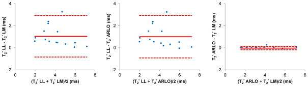
Bland-Altman plots of liver T₂^* values (in ms) obtained by mean ROI analysis over 15 liver patients at 1.5 T using the conventional log-linear (LL) and Levenberg-Marquardt (LM) methods and the proposed ARLO method (also see linear regression plots in the supplemental material).

Figure 3 shows an example of liver source images, the derived T₂^* maps, and voxel-based comparisons of the three methods using linear regression and Bland-Altman plots within one subject. Range, mean and standard deviation of T₂^* values (in ms) within the liver were [2.1 – 15.3, 4.0 ± 1.3] for LL, [2.7 – 5.3, 3.7 ± 0.3] for LM, and [2.8 – 5.6, 3.8 ± 0.3] for ARLO. Similar to the mean ROI analysis (Fig.2), LL had a rather poor linear correlation and limited agreement with both LM (R² = 0.294) and ARLO (R² = 0.194). Unlike LL, ARLO had instead an excellent linear correlation with LM (R² = 0.946, slope of regression line = 0.922) and a very narrow range of agreement (mean bias of −0.04 ms and −0.19 – 0.11 ms confidence interval) (P < 0.01).

Figure 3.

Example of a) multi-echo gradient echo source images and b) derived T₂^* maps (in ms) obtained from a patient with liver iron overload using log-linear (LL), Levenberg-Marquardt (LM) and ARLO algorithms. Note the increased noise in the map obtained with LL method. Bland-Altman plots and scatter plots (with linear regression lines) comparing liver T2^* are shown in c and d, respectively. The total fitting time of four slices for LM, LL, and ARLO was 94, 8, and 0.9 s using our Matlab implementations and 313, 26 and 2 msec using our C++ implementations.

Figure 4 shows a comparison of brain T2^* maps obtained from a healthy volunteer at 3 T. Figure 5 shows an example of cardiac T2^* maps obtained from a patient with myocardial iron overload. Using LM as the reference method, T2^* values obtained with ARLO in both the basal ganglia and the heart had a higher correlation (R² = 0.95 and 0.96, respectively) and narrower limits of agreement than that obtained with LL (R² = 0.89 and 0.80, respectively) (Figs.4&5). On the average (n=2), the processing time for the whole brain (approximately 11 million voxels) using our C++ implementations on a GE scanner was 35 sec and 9 min 15 sec for LL and LM, respectively, while ARLO took 2.7 sec.

Figure 4.

Example of a) T2^* weighted gradient echo images and b) extracted brain T₂^* maps (in ms) obtained from a healthy volunteer at 3 T using log-linear (LL), Levenberg-Marquardt (LM) and ARLO algorithms. Note the reduced T2^* in the basal ganglia due to iron storage in this area. Bland-Altman plots and scatter plots (with linear regression lines) comparing T2^* in the basal ganglia are shown in c and d, respectively. The total fitting time of this whole brain 0.7 mm isotropic 3D data set with 12 echoes (using our C++ implementations on the host computer of a GE HDxt scanner) was 41 sec and 10 min for LL and LM, respectively, while ARLO took only 3.4 sec.

Figure 5.

Example of a) T2^* weighted gradient echo images and b) cardiac T₂^* maps (in ms) obtained from a patient with myocardial iron overload at 1.5 T using log-linear (LL), Levenberg-Marquardt (LM) and ARLO algorithms. Myocardial regions with markedly decreased T2^* indicate the presence of iron (arrows). Bland-Altman plots and scatter plots (with linear regression lines) comparing myocardial T2^* are shown in c and d, respectively. The C++ fitting time for the myocardium shown in this example was 4, 0.2 and 0.02 sec for LM, LL and ARLO, respectively.

DISCUSSION

Our data demonstrate that ARLO is more robust against noise than LL in mapping T₂^*, while delivering an accuracy similar to LM. However, ARLO’s most striking improvement over the other two methods is represented by its computational speed, as ARLO proved about 100 times faster than LM and 10 times faster than LL. This characteristic allowed us to obtain an accurate whole-organ T₂^* mapping in a very short time and our in vivo evaluation in healthy volunteers and iron-overloaded patients showed that ARLO delivers T₂^* maps very similar to those obtained with LM.

The processing speed advantage can be understood in terms of computational cost estimates. ARLO uses a single-variable linear regression with a computational cost O(N), where N is the number of data points. LL uses a two-variable linear regression with a computational cost O(6N). In LM, the number of iterations needed for solving the non-linear least squares problem has a computational cost of O(N³). Thus, one expects ARLO to be faster than LL, and both ARLO and LL to be much faster than LM. Our experimental observations confirmed these predictions.

Noise propagation is a major cause of error in T₂^* mapping, particularly for iron-overloaded cases, where the short T₂^* leads to poor SNR. LL is very sensitive to noise, as its log operation amplifies noise effects (13). LM solves a non-linear least squares problem and provides the optimal maximum likelihood estimate when noise is Gaussian (18). The maximum likelihood estimate for Rician noise has been previously derived elsewhere (20). However, minimizing non-linear cost functions using iterative methods, such as LM, in the presence of noise is prone to errors due to the need for an initial guess and to convergence issues as well as requires significant computational power. ARLO provides an effective linearization of the nonlinear estimation problem, therefore providing a near-optimal solution in significantly reduced processing time. Unlike LM, ARLO provides a closed-form solution and requires simple arithmetics to compute T2^* from the multi-echo data (Eq.9). As such, ARLO does not require an initial guess and is immune to convergence issues commonly associated with iterative methods such as LM. In this study, we used the well-known Simpson rule (Eq.4) to approximate the definite integral in Eq.2. This formula is derived from a quadratic approximation and provides a 4^th order accuracy (14). By using computer simulations (data not shown), we found that this approximation provides much improved accuracy when compared to the 4^th order approximation (i.e., using the trapezoidal rule), while higher order approximations (e.g., cubic approximation using the 3/8 Simpson rule) yielded little benefit.

It is worth noticing that, in addition to integration, differentiation of Eq.1 using the central difference method is an alternative way to generate a signal magnitude time series. Higher order approximations are also possible using more points, as for example the 4^th order accuracy with 5 points (14). 1/T₂^* is obtained as the maximum-likelihood estimate of the resulting AR model. In this study, we chose integration (Eq.2) over differentiation because it provides higher accuracy with large sampling intervals and low SNRs, in agreement with error analysis of numerical implementation of integration and differentiation (14). However, with higher SNRs and adequate sampling intervals, differentiation becomes as accurate as integration (results not shown).

The integration of the signal equation with an exponential factor uniquely generates a time series, an issue that has been well studied in signal processing. Accordingly, time series analysis techniques, including auto-regression, can be applied on measured data. The exponential coefficient can be optimally determined by using the maximal likelihood estimation (17). This auto-regression on linear operations approach can also be applied for determining exponential coefficients in other MRI experiments and other signals outside MRI. ARLO applications in other MRI studies include estimating the spin-spin relaxation time T₂ from data measured at various TEs, m(t) = M₀ exp(− t/T₂); estimating off-resonance field b and $T_2^{\ast }$ from data measured at various TEs, $m(t)=M_0\mathit{exp}\left(-t(\frac{1}{T_2^{\ast }}+i\gamma b)\right)$; estimating the diffusion coefficient D from data measured at various gradient b values, m(t) = M₀ exp(−Db); and estimating the spin-lattice relaxation time T₁ from data measured at various timing parameters, such as TR or TI, m(t) = M_Z0 exp(− t/T₁) + M₀ (1− exp(− t/T₁)). For the case of $\frac{1}{T_2^{\ast }}+i\gamma b$ estimation, complex data has to be used in linear regression. For the case of T₁ estimation, which usually requires fitting a three-parameter mono-exponential model, a constant term may be needed in the linear regression. The ARLO approach may be modified to handle such constant offset, in addition to the noise baseline in the magnitude data obtained with a multiple-receiver coil, in order to avoid bias (20).

It is important to note that while the ARLO algorithm proposed in this work (Eq.9) is only suited for mono-exponential fitting, i.e., for a single chemical species, it can be generalized to handle multi-exponential or multi-spectral T2/T2^* decay data when multiple tissue compartments and/or multiple chemical species occupy the same imaging voxel, as in the case of fat and water in-voxel coexistence in the liver. However, more sophisticated fitting algorithms have been developed recently to deal with these problems (9,22,23).

A potential limitation of the method implemented in this work is the minimum detectable T2^*, which can be important for patients with severe iron overload. In our liver scans, we used a monopolar (instead of bipolar) readout gradient to avoid the time shift between even and odd echoes, resulting in an echo spacing of 1.5 ms. Furthermore, our ARLO implementation requires a minimum of 3 data points (compared to 2 by LM and LL). Our simulations indicate that these limitations in echo spacing and number of required data points result in a minimum detectable T2^* of approximately 1.5 ms by ARLO. Further reducing both the first TE and the echo spacing is therefore critical for the detection of species with very short T2^* (≤ 1.5 ms).

In conclusion, our proposed ARLO algorithm provides fast and accurate T₂^* maps and is therefore well-suited for whole-organ T₂^* mapping in iron overload diseases, besides showing potential also in other quantitative MRI studies. ARLO can replace the LL algorithm for accurate online T₂^* mapping, and replace the LM algorithm for accurate fast analysis of exponential signal behaviors.

Supplementary Material

Supp Fig S1

Figure 1 (supplemental). a) Bland-Altman plots of liver T₂^* values (in ms) obtained by mean ROI analysis over 15 liver patients at 1.5 T using the conventional log-linear (LL) and Levenberg-Marquardt (LM) methods and the proposed ARLO method. b) Corresponding scatter plots (with linear regression lines).

References

- 1.Aquino D, Bizzi A, Grisoli M, Garavaglia B, Bruzzone MG, Nardocci N, Savoiardo M, Chiapparini L. Age-related iron deposition in the basal ganglia: quantitative analysis in healthy subjects. Radiology. 2009;252:165–172. doi: 10.1148/radiol.2522081399. [DOI] [PubMed] [Google Scholar]
- 2.Ropele S, Wattjes MP, Langkammer C, Kilsdonk ID, de Graaf WL, Frederiksen JL, Fuglo D, Yiannakas M, Wheeler-Kingshott CA, Enzinger C, Rocca MA, Sprenger T, Amman M, Kappos L, Filippi M, Rovira A, Ciccarelli O, Barkhof F, Fazekas F. Multicenter R2* mapping in the healthy brain. Magn Reson Med. 2013 doi: 10.1002/mrm.24772. [DOI] [PubMed] [Google Scholar]
- 3.Khalil M, Langkammer C, Ropele S, Petrovic K, Wallner-Blazek M, Loitfelder M, Jehna M, Bachmaier G, Schmidt R, Enzinger C, Fuchs S, Fazekas F. Determinants of brain iron in multiple sclerosis: a quantitative 3T MRI study. Neurology. 2011;77:1691–1697. doi: 10.1212/WNL.0b013e318236ef0e. [DOI] [PubMed] [Google Scholar]
- 4.He T, Gatehouse PD, Smith GC, Mohiaddin RH, Pennell DJ, Firmin DN. Myocardial T2* measurements in iron-overloaded thalassemia: An in vivo study to investigate optimal methods of quantification. Magn Reson Med. 2008;60:1082–1089. doi: 10.1002/mrm.21744. [DOI] [PMC free article] [PubMed] [Google Scholar]
- 5.Carpenter JP, He T, Kirk P, Roughton M, Anderson LJ, de Noronha SV, Sheppard MN, Porter JB, Walker JM, Wood JC, Galanello R, Forni G, Catani G, Matta G, Fucharoen S, Fleming A, House MJ, Black G, Firmin DN, St Pierre TG, Pennell DJ. On T2* magnetic resonance and cardiac iron. Circulation. 2011;123:1519–1528. doi: 10.1161/CIRCULATIONAHA.110.007641. [DOI] [PMC free article] [PubMed] [Google Scholar]
- 6.Wood JC, Enriquez C, Ghugre N, Tyzka JM, Carson S, Nelson MD, Coates TD. MRI R2 and R2* mapping accurately estimates hepatic iron concentration in transfusion-dependent thalassemia and sickle cell disease patients. Blood. 2005;106:1460–1465. doi: 10.1182/blood-2004-10-3982. [DOI] [PMC free article] [PubMed] [Google Scholar]
- 7.Hankins JS, McCarville MB, Loeffler RB, Smeltzer MP, Onciu M, Hoffer FA, Li CS, Wang WC, Ware RE, Hillenbrand CM. R2* magnetic resonance imaging of the liver in patients with iron overload. Blood. 2009;113:4853–4855. doi: 10.1182/blood-2008-12-191643. [DOI] [PMC free article] [PubMed] [Google Scholar]
- 8.Henninger B, Kremser C, Rauch S, Eder R, Zoller H, Finkenstedt A, Michaely HJ, Schocke M. Evaluation of MR imaging with T1 and T2* mapping for the determination of hepatic iron overload. Eur Radiol. 2012;22:2478–2486. doi: 10.1007/s00330-012-2506-2. [DOI] [PubMed] [Google Scholar]
- 9.Taylor BA, Loeffler RB, Song R, McCarville MB, Hankins JS, Hillenbrand CM. Simultaneous field and R2 mapping to quantify liver iron content using autoregressive moving average modeling. J Magn Reson Imaging. 2012;35:1125–1132. doi: 10.1002/jmri.23545. [DOI] [PMC free article] [PubMed] [Google Scholar]
- 10.Langkammer C, Krebs N, Goessler W, Scheurer E, Ebner F, Yen K, Fazekas F, Ropele S. Quantitative MR imaging of brain iron: a postmortem validation study. Radiology. 2010;257:455–462. doi: 10.1148/radiol.10100495. [DOI] [PubMed] [Google Scholar]
- 11.Hoppe S, Quirbach S, Mamisch TC, Krause FG, Werlen S, Benneker LM. Axial T2* mapping in intervertebral discs: a new technique for assessment of intervertebral disc degeneration. Eur Radiol. 2012;22:2013–2019. doi: 10.1007/s00330-012-2448-8. [DOI] [PubMed] [Google Scholar]
- 12.Mamisch TC, Hughes T, Mosher TJ, Mueller C, Trattnig S, Boesch C, Welsch GH. T2 star relaxation times for assessment of articular cartilage at 3 T: a feasibility study. Skeletal Radiol. 2012;41:287–292. doi: 10.1007/s00256-011-1171-x. [DOI] [PubMed] [Google Scholar]
- 13.Otto R, Ferguson MR, Marro K, Grinstead JW, Friedman SD. Limitations of using logarithmic transformation and linear fitting to estimate relaxation rates in iron-loaded liver. Pediatr Radiol. 2011;41:1259–1265. doi: 10.1007/s00247-011-2082-7. [DOI] [PubMed] [Google Scholar]
- 14.Abramowitz M, Stegun IA. Handbook of mathematical functions: with formulas, graphs, and mathematical tables. xiv. New York: Dover; 1970. p. 1046. [Google Scholar]
- 15.Gudbjartsson H, Patz S. The Rician distribution of noisy MRI data. Magn Reson Med. 1995;34:910–914. doi: 10.1002/mrm.1910340618. [DOI] [PMC free article] [PubMed] [Google Scholar]
- 16.Constantinides CD, Atalar E, McVeigh ER. Signal-to-noise measurements in magnitude images from NMR phased arrays. Magn Reson Med. 1997;38:852–857. doi: 10.1002/mrm.1910380524. [DOI] [PMC free article] [PubMed] [Google Scholar]
- 17.Hamilton JD. Time series analysis. xiv. Princeton, N.J: Princeton University Press; 1994. p. 799. [Google Scholar]
- 18.Bonny JM, Zanca M, Boire JY, Veyre A. T2 maximum likelihood estimation from multiple spin-echo magnitude images. Magn Reson Med. 1996;36:287–293. doi: 10.1002/mrm.1910360216. [DOI] [PubMed] [Google Scholar]
- 19.Beaumont M, Odame I, Babyn PS, Vidarsson L, Kirby-Allen M, Cheng HL. Accurate liver T2* measurement of iron overload: a simulations investigation and in vivo study. J Magn Reson Imaging. 2009;30:313–320. doi: 10.1002/jmri.21835. [DOI] [PubMed] [Google Scholar]
- 20.Hardy PA, Andersen AH. Calculating T2 in images from a phased array receiver. Magn Reson Med. 2009;61:962–969. doi: 10.1002/mrm.21904. [DOI] [PMC free article] [PubMed] [Google Scholar]
- 21.Yin X, Shah S, Katsaggelos AK, Larson AC. Improved R2* measurement accuracy with absolute SNR truncation and optimal coil combination. NMR Biomed. 2010;23:1127–1136. doi: 10.1002/nbm.1539. [DOI] [PMC free article] [PubMed] [Google Scholar]
- 22.Yu H, Shimakawa A, McKenzie CA, Brodsky E, Brittain JH, Reeder SB. Multiecho water-fat separation and simultaneous R2* estimation with multifrequency fat spectrum modeling. Magn Reson Med. 2008;60:1122–1134. doi: 10.1002/mrm.21737. [DOI] [PMC free article] [PubMed] [Google Scholar]
- 23.Berglund J, Kullberg J. Three-dimensional water/fat separation and T2* estimation based on whole-image optimization--application in breathhold liver imaging at 1. 5 T. Magn Reson Med. 2012;67:1684–1693. doi: 10.1002/mrm.23185. [DOI] [PubMed] [Google Scholar]
Associated Data
This section collects any data citations, data availability statements, or supplementary materials included in this article.
Supplementary Materials