Impact of Correlation on Predictive Ability of Biomarkers

Summary

In this paper we investigate how the correlation structure of independent variables affects the discrimination of risk prediction model. Using multivariate normal data and binary outcome we prove that zero correlation among predictors is often detrimental for discrimination in a risk prediction model and negatively correlated predictors with positive effect sizes are beneficial. A very high multiple R-squared from regressing the new predictor on the old ones can also be beneficial. As a practical guide to new variable selection, we recommend to select predictors that have negative correlation with the risk score based on the existing variables. This step is easy to implement even when the number of new predictors is large. Our results are illustrated using real-life Framingham data suggesting that the conclusions hold outside of normality. The findings presented in this paper might be useful for preliminary selection of potentially important predictors, especially is situations where the number of predictors is large.

1. Introduction

Risk assessment plays an important role in modern clinical and preventive medicine. Lifestyle, genetic predisposition, age and medical test results affect the risk of developing a disease. Medical practitioners prescribe appropriate treatment based on this risk, while a patient can modify his or her lifestyle to mitigate the it. Statistical models are the primary tool in risk assessment. For example, in cardiovascular research, Cox regression was used to estimate the 10-year risk of coronary heart disease and the model is called the Framingham Risk Score (FRS) [1] as it was developed based on the Framingham Heart Study data [2-4]. Age, total and HDL cholesterol, systolic blood pressure, smoking status and other factors were used to predict the 10-year risk of CHD. The FRS became a routine tool in physician's offices in the US and led to the development of similar scales in other countries. In cancer research, Gail et al., [5][6] developed a model for the 5-year risk of breast cancer and it became the tool based on which high-risk patients are referred to undergo more precise but also more invasive tests. This risk score is based on a number of statistical techniques including logistic regression.

There is an ongoing search to develop new and improve existing risk prediction models. For instance, as of today original article which introduced 10-year risk model for coronary heart disease [1] was cited more than five thousand times. All these publications applied, compared or worked on improving the 10-year risk model for coronary heart disease. This quest to improve existing models is further fueled by recent advancements in genetics and modern medicine, including electronic medical record keeping. All of these result in an enormous amount of new data and consequently a large number of promising new predictors of risk. For example, in the Leukemia Microarray Study 7,128 genetic risk factors were considered as potential predictors of the outcome [7]. When the number of predictors is so large simple search for informative predictors becomes an onerous job. Therefore, it is very important to look for good predictors intelligently. We need to understand the underlying statistical principles that distinguish good predictors from those that are uninformative.

A common notion in the search for new risk markers is that variables with large univariate effect size and uncorrelated with the ones already included in the model should lead to the largest increase in model discrimination. In this paper we investigate the impact of effect size and covariance structure of predictors on discrimination in the context of multivariate normality. We show that contrary to common assumptions, correlation (especially negative correlation) between predictors can be beneficial for discrimination. We present model formulation in Section 2. In Sections 3 and 4 we show that under bivariate normality, negative conditional correlation of the two predictors leads to a more pronounced improvement in discrimination than zero conditional correlation. Furthermore, in some settings, very high positive correlation can also be beneficial. We then proceed to extend the results to the multivariate normal case and any covariance structure between predictors. In Section 5 we illustrate our findings using real-life Framingham Heart Study data and numerical simulations. We also argue that the assumption of normality may not be overly restrictive. Additional theoretical insight and generalizations of our findings are discussed in Section 6, where we also discuss practical implications of our findings.

2. Model Formulation

Let D be an outcome of interest: with D=1 for events and D=0 for non-events. Our goal is to predict the event status using p test results which we denote as x=x₁, …, x_p. Assume D and x are available for N individuals. Let P(D=1|x₁,…,x_p) denote the probability (or risk) of the outcome for each person given their risk factor status. A common choice for estimating this risk includes assuming a generalized linear model and estimating the coefficients denoted by a using logistic regression, linear discriminant analysis or other regression technique for binary outcomes. In this paper we will use the area under the receiver operating characteristics curve as a measure of the quality of the risk prediction (AUC of ROC) [8-10]. The AUC can be interpreted as the probability that a randomly selected event has a higher risk than a randomly selected non-event [11][12]. It is due to this interpretation that the AUC gained so much popularity in the field. The AUC is invariant to monotone transformations of the risk and therefore can be based on a linear combination of predictors [8], which we will call the risk score:

$$\text{rs}=\mathrm{a}\prime \mathrm{x}.$$ (1)

Suppose we want to improve the risk prediction model with p-1 predictors by adding one new predictor. We want the risk prediction model with p predictors to discriminate between the two subgroups (events versus non-events) better than the model with only the first p-1 predictors. To make theoretical developments possible, we assume multivariate normality of predictors conditional on the disease status: x|D=0 ∼ N(μ₀, Σ₀) and x|D=1 ∼ N(μ₁, Σ₁), where μ₀ and μ₁ are vectors of means for the p test results among non-events and events, respectively and Σ₀, Σ₁ are the corresponding variance-covariance matrices. We further denote differences in group means between events and non-events as Δμ = μ₁ −μ₀.

Without loss of generality we can assume that the mean differences are all non-negative:

$$\Delta \mathbf{\mu }\mathbf{\ge }\mathbf{0}.$$

This assumption will play an important role in our paper. If observed mean difference is negative we can always multiply predictor by -1.0 to assure non-negativity. Because the distribution of predictors can be quite different in the event and non-event subgroups, it is preferable to calculate all variances and covariances conditional on the event status as was done in [13]. Throughout this paper the covariance properties are described conditional on the events status.

In the next section we study factors that improve the AUC when covariance matrices are equal: Σ₀= Σ₁= Σ. We extend our results to a general case of unequal covariance matrices in the subsequent sections.

3. Improvement of Discrimination under Assumptions of Normality and Equal Covariance Matrices

Under the assumption of normality and equal covariance matrices logistic regression solution and traditional Linear Discriminant Analysis (LDA) solution converge in probability to the same mean. In addition, the LDA solution is optimal in a sense that it produces dominating ROC curve [13], it is more efficient [14] and can be written explicitly. Therefore we use the LDA as a way to construct risk scores and to derive our main results. Results are not restricted to LDA but will hold asymptotically with sample size for logistic regression. LDA allows us to write the risk scores explicitly as rs = a′x , where a is calculated as

$$\mathrm{a}=\Delta \mathrm{\mu }\prime {\sum }^{-1}.$$ (2)

The AUC of the LDA model also can also be written explicitly [13]:

$$\text{AUC}=\mathrm{\Phi }\left(\sqrt{\frac{\Delta \mathrm{\mu }\prime {\sum }^{-1}\Delta \mathrm{\mu }}{2}}\right)=\mathrm{\Phi }\left(\sqrt{\frac{{\mathrm{M}}^2}{2}}\right)$$ (3)

where Φ(·) is a standard normal cumulative distribution function and M² is the squared Mahalanobis distance - a measure of separation between two multivariate normal distributions [15]. Since the AUC is a monotone function of Mahalanobis' M² , then the AUC and M² are equivalent metrics of discrimination. Hence, we can measure improvement in discrimination either by the AUC or the Mahalanobis M².

Our ultimate goal is to evaluate factors that influence ΔAUC=ΔAUC_p -ΔAUC_p-1: improvement in the AUC after adding a new variable to p-1 predictors. Denoting squared Mahalanobis distance of the reduced and full models as M_p-1² and M_p² we can rewrite ΔAUC as:

$$\Delta \mathit{\text{AUC}}={\mathit{\text{AUC}}}_p-{\mathit{\text{AUC}}}_{p-1}=\mathrm{\Phi }\left(\sqrt{\frac{M_p^2}{2}}\right)-\mathrm{\Phi }\left(\sqrt{\frac{M_{p-1}^2}{2}}\right)=\mathrm{\Phi }\left(\sqrt{\frac{M_{p-1}^2+\Delta M^2}{2}}\right)-\mathrm{\Phi }\left(\sqrt{\frac{M_{p-1}^2}{2}}\right),$$ (4)

where we used Mahalanobis distance decomposition (M_p²=M_p-1²+ΔM², ΔM²>0) [15] to arrive at the last equality.

Note that M_p-1² does not contain any information pertinent to the new predictor variable. Thus, if the reduced model has been developed a priori and our goal is to find new predictors that improve it, the M_p-1² in (4) is predefined and we cannot do anything about it. In this situation, we need to find the mechanisms that make ΔM² as large as possible. In the Appendix we provide formal expression for ΔM² and rigorously prove all results summarized below in sections 3 through 6.

3.1 Improvement of Discrimination over a Univariate Model. Equal Covariance Matrices

First let us consider the case where p=2. In this situation we have an “old” predictor variable x₁ and we want to understand better what statistical properties of a new predictor x₂ make its contribution to the AUC as large as possible. When p=2 ΔM² can be written as (see Appendix for full derivation):

$$\Delta {\mathrm{M}}^2=\frac{{({\mathrm{\delta }}_2-\mathrm{\rho }{\mathrm{\delta }}_1)}^2}{1-{\mathrm{\rho }}^2},$$ (5)

where ρ is the correlation between x₁, x₂ conditional on event status and is the same in the two event groups and δ₁, δ₂ denote the effect sizes of the old and new predictor, respectively,

$$\mathrm{i}.\mathrm{e}.{\mathrm{\delta }}_{\mathrm{i}}=\frac{\Delta {\mathrm{\mu }}_{\mathrm{i}}}{{\mathrm{\sigma }}_{{\mathrm{x}}_{\mathrm{i}}}},\mathrm{i}=1,2.$$ (6)

Note that effect size in (6) is defined as mean difference divided by standard deviation. Throughout this paper we do not condition it on the variables already in the model as is sometimes done in the field. It allows us to express explicitly model improvement through correlation structure of the data and analyze directly the impact of the correlation structure on model performance. However for consistency of formulation [14] some parameters such as covariance structure are conditional on disease status. We address this further in Section 5. As can be seen from the Appendix, the following three factors influence improvement in discrimination:

1. Any negative correlation improves discrimination.

2. If the effect sizes of the old and new predictors are not equal, then conditional correlation sufficiently close to -1 and 1 improves discrimination. If the effect sizes are equal, then the improvement in discrimination is a decreasing function of ρ.

3. As long as δ₂, the effect size of the new predictor, satisfies δ₂>ρδ₁, its increase improved discrimination.

These results are illustrated in Figure1 where we plot the AUC of the full model as a function of the correlation between the new and old predictor. We consider three different effect sizes of the new predictor and assume that the baseline model has an AUC of 0.70. We observe that increasingly negative correlation leads to an increasing improvement in the AUC, regardless of the effect size of the added predictor. More unexpectedly, however, but consistently with formula (5), we observe that very large positive correlation can also lead to substantial increases in the AUC. We will come back to this phenomenon later. Looking at Figure 1 we also observe that there is no particular advantage to having zero correlation between predictors: the value of zero, contrary to popular perceptions in the medical literature, does not indicate a local maximum, unless we restrict our attention only to non-negative correlations. Finally, we note that for each value of the effect size in Figure 1, there is a correlation that implies no improvement in the AUC; based on formula (5), this correlation is equal to the ratio of the effect sizes.

Figure1.

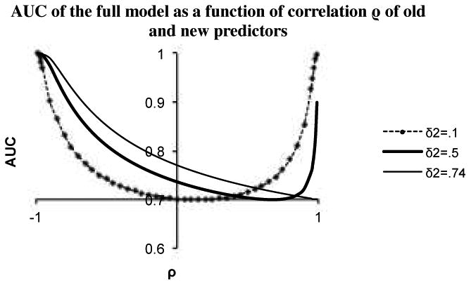
AUC of full model as function of correlation ρ of new and old predictors. New predictor is added to a model with AUC of 0.70 (δ₁=.74).

Impact of the effect size is illustrated by Figure 2. We plot the AUC of the full model as a function of the effect size of the new predictor for positive, negative and zero correlation. We note the largest gains in discrimination are achieved with negative correlation. For zero and negative correlation, the amount of increases in the AUC is a monotone function of effect size. This is not true for the positive correlation, where larger increases are observed for very small or very large effect sizes. Thus, the common notion that larger effect size must mean more improvement in discrimination is not always true. In Figure 2 AUC is a decreasing function of effect size for positive correlation if effect size is in between 0 and argmin(AUC).

Figure 2.

AUC of the full model as a function of the effect size of new predictor (δ₂). New predictor was added to a baseline model with AUC of 0.70. Correlation between old and new predictors is denoted as ρ.

We note that the results of this section are consistent with Cochran [16] who in 1964 studied factors that reduce probability of misclassification of the LDA. Because probability of misclassification is calculated as $\mathrm{P}=1-\mathrm{\Phi }\left(\frac{\sqrt{{\mathrm{M}}^2}}{2}\right)$ and $\text{AUC}=\mathrm{\Phi }\left(\sqrt{\frac{{\mathrm{M}}^2}{2}}\right)$, minimizing P is equivalent to maximizing AUC and his results could be applied to our situation.

3.3 Improvement of Discrimination over a Multivariate Model. Equal Covariance Matrices

In this section we extend the results of the previous section and that of Cochran [16] by considering the case of adding one new predictor to p-1 old predictors, p>2. We show that there exists a direct link between the improvement in discrimination and two characteristics of the new predictor: its conditional correlation with the linear predictor (or “risk score”) obtained in a model based on the first p-1 variables as well as the multiple R-square from regression of the new predictor on the first p-1 variables calculated conditional on the event status.

Without loss of generality we can assume that the new predictor has a unit variance. We show in the Appendix that ΔM² takes the form:

$$\Delta {\mathrm{M}}^2=\frac{{({\mathrm{\delta }}_{\mathrm{p}}-\text{cov}({\mathrm{x}}_{\mathrm{p}},{\text{rs}}_{\mathrm{R}}))}^2}{1-{\mathrm{R}}^2},$$ (7)

where R² is coefficient of determination obtained when regressing x_p on x₁,…, x_p-1 conditional on event status.

It follows from formula (7) that if it were possible to hold all other parameters constant, ΔM² and therefore ΔAUC, would be positively affected by:

1. Negative correlation between the new predictor and the risk score of the “old” model based on the first p-1 variables. Similarly to the univariate case, a negative association between the new predictor and the old ones is always beneficial for discrimination. In the multivariate case, the negative association is measured by the covariance of the new variable and the risk score from the model based on the first p-1 variables defined in (1). When this covariance is negative, the numerator of (5) increases, leading to improved discrimination; when the covariance is positive, its effect is detrimental to discrimination.

2. High multiple R² from the regression of the new predictor on the first p-1 variables. As the R² approaches 1, the denominator in formula (5) becomes unbounded and the improvement in discrimination measured by ΔM² increases. Because the effect of correlation in the numerator is always bounded, predictors that regress almost perfectly on the first p-1 variables have a great theoretical potential of improving model performance.

3. Effect size δ_p. This quantity is in the numerator of (5) and its increase leads to better discrimination as long as δ₂ > cov(x_p, rs_R).

Note that in order for the R² to have a discernible impact, the new predictor should regress strongly on the variables already included in the model. Based on the plot in Figure 3, R² should be roughly greater than 0.6; otherwise its effect is minimal.

Figure 3.

Effect of multiple R² on ΔM².

4. Improvement of Discrimination under Assumptions of Normality and Unequal Covariance Matrices

When covariance structure of predictors is not the same in events and non-events subgroups (Σ₀≠Σ₁) most of the results from the previous section still hold. First note that the traditional LDA solution given by (2) assumes equality or proportionality of covariance matrices. Su and Liu [13] proposed modifying the traditional LDA solution for unequal and non-proportional covariance matrices in the following way:

$$\mathrm{a}=\Delta \mathrm{\mu }\prime {({\sum }_0+{\sum }_1)}^{-1},$$ (8)

where Σ₀ and Σ₁ are variance-covariance matrices among non-events and events, respectively. They showed that the proposed solution produces the maximum AUC over all linear models and when matrices are equal or proportional, their solution (8) reduces to the traditional LDA solution given by (2).

A linear model with the coefficients estimated by (8) results in the following AUC:

$$\text{AUC}=\mathrm{\Phi }\left(\sqrt{\Delta \mathrm{\mu }\prime {({\sum }_0+{\sum }_1)}^{-1}\Delta \mathrm{\mu }}\right).$$ (9)

The right hand side of (9) can be expressed in a form similar to an equal-covariance form given in formula (3), except that the matrix Σ in (3) is replaced with the average of Σ₀ and Σ₁:

$$\text{AUC}=\mathrm{\Phi }\left(\sqrt{\frac{\Delta \mathrm{\mu }\prime {\left(\frac{{\sum }_0+{\sum }_1}{2}\right)}^{-1}\Delta \mathrm{\mu }}{2}}\right)$$ (10)

We show in the Appendix that the conclusions of previous sections can be extended to any unequal within-group covariance matrices by replacing all covariances with their averages in all formulas, including the formula (6) for calculation of effect size. First, to simplify our presentation, without the loss of generality we can assume that the new variable is always rescaled by an inverse of the square root of the average of its event group variances:

$$\frac{x}{\sqrt{\frac{{\mathrm{\sigma }}_{D=0}^2+{\mathrm{\sigma }}_{D=1}^2}{2}}}.$$

Then the following correspondence between the results for equal and unequal covariance matrices holds:

5. Connection between Covariance Matrices Conditional on Event Status and Unconditional Covariance Matrix

Results of previous sections were formulated in terms of covariance matrices of the predictors conditional on event status. However, we want to stress that conditional matrices are different from covariance matrix of the predictors calculated in the whole sample (also called unconditional variance-covariance matrix). In this section we discuss the difference between the two types of matrices and how it affects our results. In a bivariate case (p=2), if the matrices are equal, a negative correlation between predictors remains beneficial even if it is calculated in the whole sample (unconditional). In the Appendix we show that when the number of predictors p=2 and the conditional matrices are equal, the within-group ρ of Section 2 is a linearly increasing function of ρ_uncond. and negative ρ_uncond. also leads to an improvement in the AUC. In Figure 4 we plot AUC as a function of conditional and unconditional ρ.

Figure 4.

AUC as a function of conditional and unconditional correlation between new and old predictors for different effect sizes.

Figure 4 shows that in general the two correlations are different even in this simple case of a bivariate model with equal covariance matrices. This figure illustrates that general relationships discussed in previous sections from conditional case hold in the unconditional case. However in the case of more than two predictor variables there is no clear relationship and it is not possible to explicitly write the functional form when the matrices are unequal (see more details in the Appendix). This means that in general there is a fundamental difference between the two definitions and in order to correctly apply the results of this paper one must operate with conditional covariance matrices.

6. Application to Framingham Heart Study Data and Simulations

We use the Framingham Heart Study data to illustrate our findings from the previous sections. In particular, we will show situations where negative and high positive correlations are beneficial for discrimination. A total of 8,365 observations on people free of cardiovascular disease at a baseline examination in the 1970s were available. Measurements of risk factors and results of medical tests were obtained, including age, total and HDL cholesterol (tot and hdl), systolic and diastolic blood pressure (sbp and dpf). Participants of the study were followed for 12 years for the development of coronary heart disease (CHD) and were categorized as cases if they developed CHD or non-cases if they did not. To correct for skewness of the predictors simple logarithmic transformations were applied. The resulting distributions were unimodal with moderate degree of skewness; however, normality could still be rejected using the Shapiro-Wilks test [17][18]. Average of the two correlation matrices of the transformed predictors and univariate effect sizes are presented in Table 2:

Table 2.

Average of the two correlation matrices of the transformed predictors and univariate effect sizes. To satisfy assumption of non-negative effect size lnhdl was multiplied by -1 and denoted as lnhdl*.

Predictor (Effect size)	ln age (.72)	ln dpf (.42)	ln sbp (.62)	ln hdl* (.46)	ln tot (.49)
ln age	1.0	.09	.41	-.09	.25
ln dpf		1.0	.67	.06	.11
ln sbp			1.0	-.01	.15
ln hdl*				1.0	-.10
ln tot					1.0

To mimic an analysis most likely to occur in practical applications we applied logistic regression to analyze this data. Suppose we build a model “from scratch”. First, we select ln age because it has the largest univariate effect size (.72). Then, a common strategy would suggest adding ln sbp, because it has second largest effect size (.62). Addition of ln sbp increases the AUC from 0.690 to 0.713. However, using the results of Section 2 we should consider variables negatively correlated with age, namely ln hdl. This variable has a much smaller effect size (.46) yet its correlation with age is negative (-.09). Model with ln age and ln hdl has an AUC of 0.734, clearly better than the AUC of the model based on ln age and ln sbp. One might argue that ln sbp has a stronger correlation with ln age than ln hdl, so this is why the less correlated ln hdl improves discrimination by a larger amount. To illustrate that negative correlation with variables already in the model is beneficial for the improvement in the AUC we looked at the impact of a variable with the same effect size as ln hdl and the same in magnitude but opposite in direction correlation with ln age. Ln age has the same strength of correlation with ln dpf as with as ln hdl but with the opposite sign: .09 versus -.09. So ln dpf is a good candidate to illustrate the main idea. It has a smaller effect size than ln hdl, so we added a constant to it in the disorder group to match the effect size of ln hdl. Although modified ln dpf now has the same effect size as ln hdl and a similar in magnitude but opposite in direction correlation with ln age it results in the AUC of .716, still considerably smaller than the AUC of .734 obtained using the negatively correlated ln age and ln hdl. This illustrates that the negative correlation of ln hdl must play an important role in this example.

To proceed further with model building we should find new variables that are negatively correlated with the risk score (linear combination of ln age and ln hdl) and/or have a very high modified multiple R-squared. In the data described above we do not have such variables. So we decided to keep the real-life ln age and ln hdl but simulate several versions of the candidate new variables. We created the new variables as linear combinations of ln age and ln hdl plus a random normal term. We kept the effect size of the new predictor fixed at 0.60 and varied its correlation with the risk score based on the model with ln age and ln hdl. The AUCs of the model with ln age, ln hdl and the theoretical new predictor are presented below in Table 3 (recall that the AUC of the model with ln age and ln hdl is 0.734).

Table 3.

Impact of correlation on predictive ability of a new (third) biomarker. AUC is .734 for the baseline model with two predictors ln age and ln hdl.

Type of new predictor:	Univariate effect size	Correlation with the old risk score	Rsq	AUC
Uncorrelated	.60	.05	.00	.789
Negatively correlated	.60	-.70	.54	.869
Positively correlated I	.60	.73	.58	.766
Positively correlated II	.60	.91	.91	.942

Table 3 illustrates how the predictor that leads to the highest improvement in discrimination is either negatively associated with original risk score (-0.70 in row 2) or regressed on the existing variables with a very high multiple R² (0.91 in row 4). The new predictor that is uncorrelated with the existing ones in terms of R² (0.00 in row 1) produces a much smaller AUC (0.789) than the negatively associated predictor (0.869) or the predictor with a very large R² (AUC of 0.942). However, the relationship with R² is non-monotonic – looking at row 3 we notice that not sufficiently large R² is a disadvantage.

When we have repeated analysis presented in Section 6 for training (80% of the data) and validation (20% of the data) datasets, values of the AUC changed only slightly (second decimal place) and all conclusions of Section 6 remained the same (tables are available online as web-based supporting materials).

7. Discussion

In this paper we prove that for normally distributed data negative correlation between two predictors is better than zero correlation in terms of discrimination between events and non-events. Furthermore, in some settings, a new predictor that is highly correlated with the existing predictors can also lead to larger gains in discrimination.

We chose the AUC as a measure of discrimination, but the observed behavior of new predictors is not a function of this choice. It should remain true for any sensible measure of discrimination. This can be seen from the following plots in Figure 7. In this figure we present a number of scatterplots of x versus y which represent two multivariate normal random variables with conditional distributions given by (x, y)|D=0 ∼ N(0,Σ) and (x, y)|D=1 ∼ N(δ,Σ). We consider δ=(1.5, 0.6) and different variance-covariance matrices Σ, which lead to conditional (on D) correlations ρ equal to 0, -0.85 and 0.98. Events (D=1) are marked as dots and non-events (D=0) as circles. We note that for ρ=0 dots and circles form two round clouds with substantial overlap. As ρ changes, the two clouds become ellipsoidal and for ρ=-0.85 we see almost compete separation between them. We need a higher positive correlation in order to achieve the same effect of almost perfect separation. The scatterplot for ρ=0.98 demonstrates separation comparable to what is seen when ρ=-0.85.

This topic has been studied before. Mardia et al. [15] observed that correlation improved discrimination in the bivariate normal case. The same issue was discussed by Cochran, (1964)[16], but both did it in terms of the probability of misclassification. Our paper addresses how those results are related to the improvement in model discrimination as quantified by the AUC and extends the earlier results to the multivariate normal case and unequal covariance matrices. Further research is needed to extend these results rigirously beyond normality. However, it can be argued that any continuous predictor can be transformed to have its distribution approximate normality, so our assumption is not prohibitively restrictive in this case. Furthermore, our example using Framingham Heart Study data with variables that were not normal suggested that the results seem to hold if normality is not grossly violated. This suggestion needs to be verified by simulations.

It is essential to note that our findings are theoretical in nature and they intend to point out that the correlation and effect size between the new predictor and the existing variables have a more complicated relationship with improvement in discrimination. The popular notion that no correlation and high effect size offer all that we need is not true. However, this simple notion may not be far off from the truth, when we are willing to restrict our attention to non-negative correlations and sufficiently large effect sizes. We see in Figure 1 that for effect sizes of 0.5 or 0.74 and correlations between 0 and 0.6, the improvement in discrimination decreases as a function of correlation. On the other hand, in Figure 2, we observe that for correlations that are not overly large, the improvement increases as a function of effect size. These effect sizes and limited correlations are the most likely scenarios occurring in practice.

Our findings, however, offer new directions in the search for novel predictors. While it may be extremely difficult to identify variables with extremely large correlations and different effect sizes (we had to simulate them ourselves), finding predictors with negative correlation need not be as formidable. As seen in our example with hdl, even small amount of negative correlation can lead to a noticeable improvement in discrimination. Thus identification of predictors that correlate negatively with the existing risk factors and retain sufficient strength of association with the outcome may be the most promising direction in the search for new markers.

Figure 5.

Scatterplots of x₁ and x₂ for different correlations between x₁ and x₂. Pluses are events and circles are non-events.

Table 1.

Summary of Factors that Improve Model Performance.

cov_D=0(x_p, rs_R) and cov_D=1(x_p, rs_R) is covariance between new predictor and the old risk score calculated separately among non-events and events respectively δ_p is effect size calculated with respect to the average of variances:

$${\mathrm{\delta }}_{\mathrm{p}}=\frac{\Delta {\mathrm{\mu }}_2}{\sqrt{\frac{{\text{var}}_{\mathrm{D}=0}({\mathrm{x}}_{\mathrm{p}})+{\text{var}}_{\mathrm{D}=1}({\mathrm{x}}_{\mathrm{p}})}{2}}}=\frac{\Delta {\mathrm{\mu }}_2}{\sqrt{\overline{\text{var}}({\mathrm{x}}_{\mathrm{p}})}}$$

Factors that Improve Model Performance for
Equal Covariance Matrices	Unequal Covariance Matrices
1. cov(xp,rsp-1)<0	1. $\frac{\text{cov}{({\mathrm{x}}_{\mathrm{p}},{\text{rs}}_{\mathrm{p}-1})}_{\mathrm{D}=0}+\text{cov}{({\mathrm{x}}_{\mathrm{p}},{\text{rs}}_{\mathrm{p}-1})}_{\mathrm{D}=1}}{2}<0$
2. High multiple R2 of regressing xp on (x1, …, xp-1).	2. High modified R2 – see Appendix for the formula.
3. High δp provided δp>cov(xp, rsR)	3. High δp provided ${\mathrm{\delta }}_{\mathrm{p}}>\frac{\text{cov}{({\mathrm{x}}_{\mathrm{p}},{\text{rs}}_{\mathrm{p}-1})}_{\mathrm{D}=0}+cov{({\mathrm{x}}_{\mathrm{p}},{\text{rs}}_{\mathrm{p}-1})}_{\mathrm{D}=1}}{2}$

Appendix

Notation

A disease status D and p medical test results are available for N patients. We denote test results as x=x₁, …, x_p. We assume multivariate normality of test results conditional on the disease status: x|D=0 ∼ N(μ₀, Σ₀) and x|D=1 ∼ N(μ₁, Σ₁), where μ₀ and μ₁ are vectors of means for the p test results among non-events and events, respectively and Σ₀, Σ₁ are the variance-covariance matrices of the predictor in the subgroups of non-events and events correspondingly. We further denote differences in group means between events and non-events as Δμ = μ₁ − μ₀ and assume that mean differences are all non-negative: Δμ ≥0. Our goal is to evaluate improvement in the AUC after adding the p-th variable to the first p-1 variables. We can write any variance-covariance matrix Σ as: $\sum =\left[\begin{array}{c}{\sum }_{11}{\sum }_{12}\\ {\sum }_{21}{\sum }_{22}\end{array}\right]$, where Σ₁₁ is the variance-covariance matrix for the first p-1 predictors, Σ₁₂ is the covariance matrix of the first p-1 predictors with the new predictor and Σ₂₂ is the variance of the new predictor. Δμ can be written as $\left[\begin{array}{c}\Delta {\mathrm{\mu }}_1\\ \Delta {\mathrm{\mu }}_2\end{array}\right]$, where Δμ₁ is the vector of differences in the means of the first p-1 predictors and Δμ₂ is the difference of means of the new predictor.

Part 1. Equal variance-covariance matrices (Σ₀= Σ₁= Σ)

A1. Mahalanobis Distance Decomposition [15]

Using the notation of Section 2, the Mahalanobis distance of the full model based on all p predictors $({\mathrm{M}}_{\mathrm{p}}^2)$ can be written as a function of the corresponding distance for the first p-1 variables $\left({\mathrm{M}}_{\mathrm{p}-1}^2\right)$ plus an increment (ΔM²):

$$\begin{array}{l}{\mathrm{M}}_{\mathrm{p}}^2=\Delta \mathrm{\mu }\prime {\sum }^{-1}\Delta \mathrm{\mu }=\Delta {\mathrm{\mu }}_1^{\prime }{\sum }^{-1}\Delta {\mathrm{\mu }}_1+{(\Delta {\mathrm{\mu }}_2-{\sum }_{21}{\sum }_{11}^{-1}\Delta {\mathrm{\mu }}_1)}^{\prime }{({\sum }_{22}-{\sum }_{21}{\sum }_{11}^{-1}{\sum }_{12})}^{-1}(\Delta {\mathrm{\mu }}_2-{\sum }_{21}{\sum }_{11}^{-1}\Delta {\mathrm{\mu }}_1)={\mathrm{M}}_{\mathrm{p}-1}^2+\Delta {\mathrm{M}}^2,\\ \text{where}\Delta {\mathrm{M}}^2={(\Delta {\mathrm{\mu }}_2-{\sum }_{21}{\sum }_{11}^{-1}\Delta {\mathrm{\mu }}_1)}^{\prime }{({\sum }_{22}-{\sum }_{21}{\sum }_{11}^{-1}{\sum }_{12})}^{-1}(\Delta {\mathrm{\mu }}_2-{\sum }_{21}{\sum }_{11}^{-1}\Delta {\mathrm{\mu }}_1)\end{array}$$ (a1)

A2. ΔM² when p=2

When p=2, then we can simplify (a1) because Σ₁₁=var x₁, Σ₂₂=var x₂, Σ₁₂=cov(x₁, x₂):

$$\Delta {\mathrm{M}}^2=\frac{{(\Delta {\mathrm{\mu }}_2-\frac{\text{cov}({\mathrm{x}}_1,{\mathrm{x}}_2)}{\text{var}{\mathrm{x}}_1}\Delta {\mathrm{\mu }}_1)}^2}{\text{var}{\mathrm{x}}_2-\frac{{\text{cov}}^2({\mathrm{x}}_1,{\mathrm{x}}_2)}{\text{var}{\mathrm{x}}_1}}=\frac{{({\mathrm{\delta }}_2-\mathrm{\rho }{\mathrm{\delta }}_1)}^2}{1-{\mathrm{\rho }}^2},$$ (a2)

where ρ=corr(x₁, x₂).

Therefore improvement in the AUC is fully defined by (a2) which is a function of effect size and correlation coefficient of the old and new predictor variables.

A3. Conditions of improvement in AUC when p=2

Let us investigate the behavior of ΔM² defined in (a2) as function of ρ and effect size δ₂.

Improvement in AUC as a function of ρ

The first derivative of ΔM² with respect to ρ is:

$${(\Delta {\mathrm{M}}^2)}_{\mathrm{\rho }}^{\prime }={\left(\frac{{({\mathrm{\delta }}_2-{\mathrm{\delta }}_1\mathrm{\rho })}^2}{1-{\mathrm{\rho }}^2}\right)}_{\mathrm{\rho }}^{\prime }=\frac{2({\mathrm{\delta }}_2-{\mathrm{\delta }}_1\mathrm{\rho })({\mathrm{\delta }}_2\mathrm{\rho }-{\mathrm{\delta }}_1)}{{(1-{\mathrm{\rho }}^2)}^2}$$

There are two possible cases:

Case 1. δ₂≠δ₁:

The first derivative is zero when $\mathrm{\rho }=\{\begin{array}{c}{\mathrm{\delta }}_1/{\mathrm{\delta }}_2,\text{if}{\mathrm{\delta }}_1<{\mathrm{\delta }}_2\\ {\mathrm{\delta }}_2/{\mathrm{\delta }}_1,\text{if}{\mathrm{\delta }}_2<{\mathrm{\delta }}_1\end{array}$ and changes sign from negative to positive as we approach the root from left to right. Therefore, ΔM² is a convex function with a minimum at the specified values of ρ. Minimum is attained at the positive value of ρ, and hence any negative ρ is better for discrimination than ρ=0.

Case 2. δ₂=δ₁=δ

In this case ΔM² reduces to:

$$\Delta {\mathrm{M}}^2=\frac{{({\mathrm{\delta }}_2-{\mathrm{\delta }}_1\mathrm{\rho })}^2}{1-{\mathrm{\rho }}^2}=\frac{{\mathrm{\delta }}^2(1-\mathrm{\rho })}{1+\mathrm{\rho }}$$

Its first derivative is equal to $\frac{-2{\mathrm{\delta }}^2}{{(1+\mathrm{\rho })}^2}$ and it is always negative. Therefore ΔM² is a decreasing function of ρ.

Therefore, the following statements describe improvement in discrimination as measured by ΔM²:

1. If δ₁≠δ₂ then ΔM² is convex in terms of ρ. It achieves its minimum at ρ=δ₂/δ₁ or ρ=δ₁/δ₂ (if δ₂<δ₁ or δ₁<δ₂, correspondingly) and achieves its maximum as ρ→±1.

2. If δ₁=δ₂ then ΔM² is monotone decreasing in ρ.

3. If ρ<0 as ρ→-1 both numerator and denominator contribute to the growth of ΔM². Indeed as ρ gets closer to -1, the numerator is increasing and the denominator is decreasing which creates synergistic effect on the growth of ΔM². This is different when ρ>0. As positive ρ increases, both the denominator and numerator decrease. Therefore, any negative correlation is beneficial and also ΔM² improves at a faster rate for negative correlation than for positive correlation.

Improvement in AUC as a function of effect size of new predictor

Let us investigate the behavior of function $\Delta {\mathrm{M}}^2=\frac{{({\mathrm{\delta }}_2-{\mathrm{\delta }}_1\mathrm{\rho })}^2}{1-{\mathrm{\rho }}^2}$ as a function of the effect size of the new predictor δ₂. ΔM² is a quadratic function with respect to δ₂ with the minimum attained at δ₂=δ₁ρ. If δ₂<δ₁ρ, the derivative of ΔM² with respect to δ₂ is negative and we observe a paradoxical behavior when ΔM² is a decreasing function of the effect size of the new variable and a larger effect size δ₂ translates into a smaller improvement in the AUC. This unexpected behavior is illustrated in Figure 2. If δ₂>δ₁ρ then the derivative is positive and the larger effect size is beneficial.

A4. Improvement in AUC when p>2

Without loss of generality we can assume that the new predictor x_p has a unit variance. Therefore Σ₂₂=1 and the difference of means of the new variable equals its effect size, Δμ₂=δ_p.

Statement

When p>2, $\Delta {\mathrm{M}}^2=\frac{{({\mathrm{\delta }}_{\mathrm{p}}-\text{cov}({\mathrm{x}}_{\mathrm{p}},{\text{rs}}_{\mathrm{p}-1}))}^2}{1-{\mathrm{R}}^2}$, where cov(x_p, rs_p−1) is the covariance between the new predictor and the old risk score from the model based on the first p-1 variables and R² is the coefficient of determination from a multiple regression of x_p on x₁,…, x_p-1 conditional on events status.

Proof

Indeed, when p>2 ΔM² can be written as:

$$\Delta {\mathrm{M}}^2=\frac{{({\mathrm{\delta }}_{\mathrm{p}}-{\sum }_{21}{\sum }_{11}^{-1}\Delta {\mathrm{\mu }}_1)}^2}{1-{\sum }_{21}{\sum }_{11}^{-1}{\sum }_{12}}$$ (a3)

We note that if rs_p-1 is the risk score based on the reduced model then:

$$\begin{array}{l}\text{cov}(x_p,{\mathit{\text{rs}}}_{p-1})=\text{cov}(x_p,\Delta {\mathrm{\mu }}_1^{\prime }{\sum }_{11}^{-1}(x_1,\dots ,x_{p-1})\prime )=\Delta {\mathrm{\mu }}_1^{\prime }{\sum }_{11}^{-1}\text{cov}(x_p,(x_1,\dots ,x_{p-1})\prime )=\Delta {\mathrm{\mu }}_1^{\prime }{\sum }_{11}^{-1}{\sum }_{12}={\sum }_{21}{\sum }_{11}^{-1}\Delta {\mathrm{\mu }}_1\end{array}$$ (a4)

Also $1-{\sum }_{21}{\sum }_{11}^{-1}{\sum }_{12}=1-R^2$, see [20].

Hence, we can rewrite (a1) as:

$$\begin{array}{l}\Delta {\mathrm{M}}^2=\frac{{({\mathrm{\delta }}_{\mathrm{p}}-\text{cov}({\mathrm{x}}_{\mathrm{p}},{\text{rs}}_{\mathrm{p}-1}))}^2}{1-{\mathrm{R}}^2}\\ \mathrm{q}.\mathrm{e}.\mathrm{d}.\end{array}$$

Part 2. Unequal variance-covariance matrices

A5. Mahalanobis Distance Decomposition when Σ₀≠Σ₁

Su and Liu's solution [13], a = Δμ′(Σ₀ + Σ₁)⁻¹ is optimal for linear models when predictors have different variance-covariance structure in event and non-event groups. This solution produces AUC that can be written as in (8): $\text{AUC}=\left(\sqrt{\Delta \mu \prime {({\sum }_0+{\sum }_1)}^{-1}\Delta \mu }\right)$. We still can apply Mahalanobis distance decomposition to Δμ′(Σ₀ + Σ₁)⁻¹ Δμ as was shown in Appendix of [19]. Therefore improvement in the AUC is again fully defined by the improvement in the ΔM² which can be written in the following way:

$$\begin{array}{l}{\mathrm{M}}_{\mathrm{p}}^2=\Delta \mathrm{\mu }\prime {\overline{\sum }}^{-1}\Delta \mathrm{\mu }={\left[\begin{array}{c}\Delta {\mathrm{\mu }}_1\\ \Delta {\mathrm{\mu }}_2\end{array}\right]}^{\prime }{\left[\begin{array}{c}{\overline{\sum }}_{11}{\overline{\sum }}_{12}\\ {\overline{\sum }}_{21}{\overline{\sum }}_{22}\end{array}\right]}^{-1}\left[\begin{array}{c}\Delta {\mathrm{\mu }}_1\\ \Delta {\mathrm{\mu }}_2\end{array}\right]=\\ \Delta {\mathrm{\mu }}_1^{\prime }{\overline{\sum }}_{11}^{-1}\Delta {\mathrm{\mu }}_1+{(\Delta {\mathrm{\mu }}_2-{\overline{\sum }}_{21}{\overline{\sum }}_{11}^{-1}\Delta {\mathrm{\mu }}_1)}^{\prime }{({\overline{\sum }}_{22}-{\overline{\sum }}_{21}{\overline{\sum }}_{11}^{-1}{\overline{\sum }}_{12})}^{-1}(\Delta {\mathrm{\mu }}_2-{\overline{\sum }}_{21}{\overline{\sum }}_{11}^{-1}\Delta {\mathrm{\mu }}_1)={\mathrm{M}}_{\mathrm{p}-1}^2+\Delta {\mathrm{M}}^2,\\ \text{where}{\overline{\sum }}_{\text{ij}}=\frac{{\sum }_{\text{ij}}^{\mathrm{D}=0}+{\sum }_{\text{ij}}^{\mathrm{D}=1}}{2}\mathrm{i},\mathrm{j}=1,2\end{array}$$

To simplify calculations we assume that the new predictor is rescaled by the inverse of the average of the two within-group variances. Therefore, we without the loss of generality we can assume that Σ₂₂=1. Because within group matrices are unequal, we suggest defining effect size as the ratio of mean difference to the square of the average variance: $\sqrt{\overline{\text{var}}{\mathrm{x}}_{\mathrm{p}}}=\sqrt{\frac{{\text{var}}_{\mathrm{D}=0}{\mathrm{x}}_{\mathrm{p}}+{\text{var}}_{\mathrm{D}=1}{\mathrm{x}}_{\mathrm{p}}}{2}}$. Then mean difference of the rescaled new predictor and its effect size are equal: Δμ₂=δ_p. Therefore we can write ΔM² as:

$$\Delta {\mathrm{M}}^2={({\mathrm{\delta }}_{\mathrm{p}}-{\overline{\sum }}_{21}{\overline{\sum }}_{11}^{-1}\Delta {\mathrm{\mu }}_1)}^{\prime }{(1-{\overline{\sum }}_{21}{\overline{\sum }}_{11}^{-1}{\overline{\sum }}_{12})}^{-1}({\mathrm{\delta }}_{\mathrm{p}}-{\overline{\sum }}_{21}{\overline{\sum }}_{11}^{-1}\Delta {\mathrm{\mu }}_1)$$ (a5)

A6. Improvement in AUC when p=2

When p=2, then ${\overline{\sum }}_{12}=\frac{1}{2}(\text{cov}{({\mathrm{x}}_1,{\mathrm{x}}_2)}_{\mathrm{D}=0}+\text{cov}{({\mathrm{x}}_1,{\mathrm{x}}_2)}_{\mathrm{D}=1})=\overline{\text{cov}}({\mathrm{x}}_1,{\mathrm{x}}_2)$, and we can rewrite (a5) as $\Delta {\mathrm{M}}^2=\frac{{({\mathrm{\delta }}_2-{\mathrm{\delta }}_1\overline{\text{cov}}({\mathrm{x}}_1,{\mathrm{x}}_2))}^2}{1-{\overline{\text{cov}}}^2({\mathrm{x}}_1,{\mathrm{x}}_2)}$.

A7. Conditions for improvement of AUC when p=2

All conclusions of A3 hold for unequal covariance matrices once ρ is replaced with $\overline{\text{cov}}({\mathrm{x}}_1,{\mathrm{x}}_2)$.

A8. Improvement of AUC when p>2

Statement

$$\text{If p}>2,\Delta {\mathrm{M}}^2=\frac{{({\mathrm{\delta }}_{\mathrm{p}}-\frac{\text{cov}{({\mathrm{x}}_{\mathrm{p}},{\text{rs}}_{\mathrm{p}-1})}_{\mathrm{D}=0}+\text{cov}{({\mathrm{x}}_{\mathrm{p}},{\text{rs}}_{\mathrm{p}-1})}_{\mathrm{D}=1}}{2})}^2}{1-{\mathrm{R}}^2\ast },$$ (a6)

where ${\mathrm{R}}^2\ast ={\overline{\sum }}_{21}{\overline{\sum }}_{11}^{-1}{\overline{\sum }}_{12}$.

Proof

When p>2 ΔM² in (a5) can be written as:

$$\Delta {\mathrm{M}}^2=\frac{{({\mathrm{\delta }}_{\mathrm{p}}-{\overline{\sum }}_{21}{\overline{\sum }}_{11}^{-1}\Delta {\mathrm{\mu }}_1)}^2}{1-{\overline{\sum }}_{21}{\overline{\sum }}_{11}^{-1}{\overline{\sum }}_{12}}$$ (a7)

Let us show that ${\overline{\sum }}_{21}{\overline{\sum }}_{11}^{-1}\Delta {\mathrm{\mu }}_1=\overline{\text{cov}}({\mathrm{x}}_{\mathrm{p}},{\text{rs}}_{\mathrm{p}-1})$. Conditioning on non-events groups we can write:

$${\text{cov}}_0({\mathrm{x}}_{\mathrm{p}},{\text{rs}}_{\mathrm{p}-1})={\text{cov}}_0({\mathrm{x}}_{\mathrm{p}},\Delta \mathrm{\mu }\prime {\overline{\sum }}_{11}^{-1}({\mathrm{x}}_1,\dots ,{\mathrm{x}}_{\mathrm{p}-1})\prime )=\Delta {\mathrm{\mu }}_1^{\prime }{\overline{\sum }}_{11}^{-1}{\text{cov}}_0({\mathrm{x}}_{\mathrm{p}},({\mathrm{x}}_1,\dots ,{\mathrm{x}}_{\mathrm{p}-1})\prime )=\Delta {\mathrm{\mu }}_1^{\prime }{\overline{\sum }}_{11}^{-1}{\sum }_{12}^{\mathrm{D}=0}={\sum }_{21}^{\mathrm{D}=0}{\overline{\sum }}_{11}^{-1}\Delta {\mathrm{\mu }}_1$$

Similarly among events ${\text{cov}}_1({\mathrm{x}}_{\mathrm{p}},{\text{rs}}_{\mathrm{p}-1})={\sum }_{21}^{\mathrm{D}=1}{\overline{\sum }}_{11}^{-1}\Delta {\mathrm{\mu }}_1$.

Thus $\frac{{\text{cov}}_0({\mathrm{x}}_{\mathrm{p}},{\text{rs}}_{\mathrm{p}-1})+{\text{cov}}_1({\mathrm{x}}_{\mathrm{p}},{\text{rs}}_{\mathrm{p}-1})}{2}=\frac{({\sum }_{21}^{\mathrm{D}=0}+{\sum }_{21}^{\mathrm{D}=1})}{2}{\overline{\sum }}_{11}^{-1}\Delta {\mathrm{\mu }}_1\stackrel{\text{def}}{=}{\overline{\sum }}_{21}{\overline{\sum }}_{11}^{-1}\Delta {\mathrm{\mu }}_1$.

$1-{\overline{\sum }}_{21}{\overline{\sum }}_{11}^{-1}{\overline{\sum }}_{12}$ in the denominator of (a7) resembles formula (a4) for multiple regression R², except the covariance matrices in it should be replaced by the average of covariance matrices in the two subgroups. So by analogy to (a3) we define it as R²* - modified multiple R². Hence, we can rewrite (a7) as:

$$\begin{array}{l}\Delta {\mathrm{M}}^2=\frac{{({\mathrm{\delta }}_{\mathrm{p}}-\overline{\text{cov}({\mathrm{x}}_{\mathrm{p}},{\text{rs}}_{\mathrm{p}-1})})}^2}{1-{\mathrm{R}}^2\ast }\\ \mathrm{q}.\mathrm{e}.\mathrm{d}.\end{array}$$

A9. Correlation conditional on event status versus correlation calculated among non-events and events pooled together

If a model has two predictors with equal covariance structure within event and non-event categories, there exists a relationship between the two types of covariances.

$$\text{Let}{\left[\begin{array}{c}{x}_1\\ x_2\end{array}\right]}_{D=0}\sim N(0,[\begin{array}{c}{\mathrm{\sigma }}_1^2{\mathrm{\sigma }}_{12}\\ {\mathrm{\sigma }}_{12}{\mathrm{\sigma }}_2^2\end{array}\left]\right),{\left[\begin{array}{c}{x}_1\\ x_2\end{array}\right]}_{D=1}\sim N\left(\right[\begin{array}{c}\Delta {\mathrm{\mu }}_1\\ \Delta {\mathrm{\mu }}_2\end{array}],[\begin{array}{c}{\mathrm{\sigma }}_1^2{\mathrm{\sigma }}_{12}\\ {\mathrm{\sigma }}_{12}{\mathrm{\sigma }}_2^2\end{array}\left]\right)$$

Denote the fraction of events as π and E_D=0=E₀, E_D=1=E₁. Covariance calculated in a sample which pools events and non-events is:

$$\begin{array}{l}\text{cov}(x_1,x_2)=E(x_1{x}_2)-E{x}_{1}E{x}_2\\ \text{Because}{E}_0(x_1{x}_2)={\mathrm{\sigma }}_{12}\text{and}{E}_1(x_1{x}_2)={\mathrm{\sigma }}_{12}+\Delta {\mathrm{\mu }}_1\Delta {\mathrm{\mu }}_2,\\ E(x_1{x}_2)=(1-\pi )E_0(x_1{x}_2)+\pi E_1(x_1{x}_2)={\mathrm{\sigma }}_{12}+\pi \Delta {\mathrm{\mu }}_1\Delta {\mathrm{\mu }}_2\\ E{x}_{1}E{x}_2={\pi }^2\Delta {\mathrm{\mu }}_1\Delta {\mathrm{\mu }}_2\\ \text{So cov}(x_1,x_2)={\mathrm{\sigma }}_{12}+\pi (1-\pi )\Delta {\mathrm{\mu }}_1\Delta {\mathrm{\mu }}_2\end{array}$$

Since $\text{var}{x}_1={\mathrm{\sigma }}_1^2+\pi (1-\pi )\Delta {\mathrm{\mu }}_1^2$, $\text{var}{x}_2={\mathrm{\sigma }}_2^2+\pi (1-\pi )\Delta {\mathrm{\mu }}_2^2$,

$${\mathrm{\rho }}_{\mathit{\text{mixed}}}=\frac{{\mathrm{\sigma }}_{12}+\pi (1-\pi )\Delta {\mathrm{\mu }}_1\Delta {\mathrm{\mu }}_2}{\sqrt{\text{var}{x}_1\text{var}{x}_2}}=\frac{\mathrm{\rho }+\pi (1-\pi ){\mathrm{\delta }}_1{\mathrm{\delta }}_2}{\sqrt{(1+\pi (1-\pi ){\mathrm{\delta }}_1)(1+\pi (1-\pi ){\mathrm{\delta }}_2)}},$$ (a8)

where ρ_D=0= ρ_D=1= ρ is the correlation coefficient between x₁ and x₂ conditional on event status. It follows from (a8) that unconditional correlation is a linear increasing function of within group correlation coefficient ρ. However there is no such clear relationship when the number of predictors is greater than two nor for unequal covariance matrices.

References

- 1.Wilson PWF, D'Agostino RB, Levy D, Belanger AM, Silbershatz H, Kannel WB. Prediction of coronary heart disease using risk factor categories. Circulation. 1998;97:1837–1847. doi: 10.1161/01.cir.97.18.1837. [DOI] [PubMed] [Google Scholar]
- 2.Anderson KM, Odell PM, Wilson PWF, Kannel WB. Cardiovascular disease risk profiles. American Heart Journal. 1991;121:293–298. doi: 10.1016/0002-8703(91)90861-b. [DOI] [PubMed] [Google Scholar]
- 3.D'Agostino RB, Vasan RS, Pencina MJ, Wolf PA, Cobain MR, Massaro JM, Kannel WB. General Cardiovascular Risk Profile for Use in Primary Care: The Framingham Heart Study. Circulation. 2008;117:743–753. doi: 10.1161/CIRCULATIONAHA.107.699579. [DOI] [PubMed] [Google Scholar]
- 4.Grundy SM, Becker D, Clark LT, Cooper RS, Denke MA, Howard WJ, et al. Executive Summary of the Third Report of the National Cholesterol Education Program (NCEP) Expert Panel on Detection, Evaluation and Treatment of High Blood Cholesterol in Adults (Adult Treatment Panel III) Journal of the American Medical Association. 2001;285:2486–2497. doi: 10.1001/jama.285.19.2486. [DOI] [PubMed] [Google Scholar]
- 5.Gail MH, Brinton LA, Byar DP, Corle DK, Green SB, Schairer C, Mulvihill JJ. Projecting Individualized Probabilities of Developing Breast Cancer for White Females Who Are Being Examined Annually. Journal of the National Cancer Institute. 1989;81:1879–1886. doi: 10.1093/jnci/81.24.1879. [DOI] [PubMed] [Google Scholar]
- 6.Gail MH, Costantino JP, Pee D, Bondy M, Newman L, Selvan M, Anderson GL, Malone KE, Marchbanks PA, McCaskill-Stevens W, Norman SA, Simon MA, Spirtas R, Ursin G, Bernstein L. Projecting individualized absolute invasive breast cancer risk in African American women. Journal of the National Cancer Institute. 2007;99(23):1782–1792. doi: 10.1093/jnci/djm223. [DOI] [PubMed] [Google Scholar]
- 7.Golub TR, Slonim DK, Tamayo P, Huard C, Gaasenbeek M, Mesirov JP, Coller H, Loh ML, Downing JR, Caligiuri MA, Bloomfield CD, Lander ES. Molecular Classification of Cancer: Class Discovery and Class Prediction by Gene Expression Monitoring. Science. 1999;286(5439):531–537. doi: 10.1126/science.286.5439.531. [DOI] [PubMed] [Google Scholar]
- 8.Pepe MS. The Statistical Evaluation of Medical Tests for Classification and Prediction. Oxford University Press; 2004. pp. 77–79. [Google Scholar]
- 9.D'Agostino RB, Griffith JL, Schmidt CH, Terrin N. Measures for evaluating model performance. Proceedings of the biometrics section. American Statistical Association, Biometrics Section; Alexandria, VA. U.S.A.. 1997; pp. 253–258. [Google Scholar]
- 10.Harrel FE. Tutorial in biostatistics: multivariable prognstic models: issues in developing models, evaluating assumptions and adequacy, and measuring and reducing errors. Statistics in Medicine. 1996;15:361–387. doi: 10.1002/(SICI)1097-0258(19960229)15:4<361::AID-SIM168>3.0.CO;2-4. [DOI] [PubMed] [Google Scholar]
- 11.Bamber D. The area above the ordinal dominance graph and the area below the receiver operating characteristic graph. Journal of Mathematical Psychology. 1975;12:387–415. [Google Scholar]
- 12.Hanley JA, McNeil BJ. The meaning and use of the area under a receiver operating characteristic (ROC) curve. Radiology. 1982;143:29–36. doi: 10.1148/radiology.143.1.7063747. [DOI] [PubMed] [Google Scholar]
- 13.Su JQ, Liu JS. Linear combinations of multiple diagnostic markers. Journal of American Statistical Association. 1993;88(424):1350–1355. [Google Scholar]
- 14.Efron B. The Efficiency of Logistic Regression Compared to Normal Discriminant Analysis. Journal of American Statistical Association. 1973;70(352):892–898. [Google Scholar]
- 15.Mardia KV, Kent JT, Bibby JM. Multivariate Analasys. Academic Press; 1979. [Google Scholar]
- 16.Cochran WG. On the Performance of the Linear Discriminant Function. Technometrics. 1964;6(2):179–190. [Google Scholar]
- 17.Shapiro SS, Wilk MB. An Analysis of Variance Test for Normality (Complete Samples) Biometrika. 1965;52(34):591–611. [Google Scholar]
- 18.Pearson ES, D'Agostino RB, Bowman RO. Tests for Departure from Normality Comparison of Powers. Biometrika. 1977;64(2):231–246. [Google Scholar]
- 19.Demler OV, Pencina MJ, D'Agostino RB., Sr Equivalence of improvement in area under ROC curve and linear discriminant analysis coefficient under assumption of normality. Statistics in Medicine. 2011;30(12):1410–1418. doi: 10.1002/sim.4196. [DOI] [PubMed] [Google Scholar]
- 20.Weisberg S. Applied Linear Regression. John Wiley and Sons; New Jersey: 2005. pp. 62–64. [Google Scholar]
Associated Data
This section collects any data citations, data availability statements, or supplementary materials included in this article.