Comparative Study of Computational Methods for Reconstructing Genetic Networks of Cancer-Related Pathways

Abstract

Network reconstruction is an important yet challenging task in systems biology. While many methods have been recently proposed for reconstructing biological networks from diverse data types, properties of estimated networks and differences between reconstruction methods are not well understood. In this paper, we conduct a comprehensive empirical evaluation of seven existing network reconstruction methods, by comparing the estimated networks with different sparsity levels for both normal and tumor samples. The results suggest substantial heterogeneity in networks reconstructed using different reconstruction methods. Our findings also provide evidence for significant differences between networks of normal and tumor samples, even after accounting for the considerable variability in structures of networks estimated using different reconstruction methods. These differences can offer new insight into changes in mechanisms of genetic interaction associated with cancer initiation and progression.

Introduction

An important goal of genomics is to understand the relationship among genes, characterized by the regulation and synthesis of proteins as reactions to internal and external signals. These relationships can be concisely represented in a gene network, where nodes are genes and edges between them capture interactions at different levels, for instance, interactions between corresponding proteins or a protein and a messenger RNA.

Edges in a gene network can be either directed or undirected. A directed edge often represents a causal effect of one gene to another, for example in the case of transcriptional protein–DNA interactions.^1–3 An undirected edge, on the other hand, represents an association between two genes, for instance in the case of protein–protein interactions.^3–5

Genetic interactions cast new insights into activities of biological pathway and cellular response,^6,7 and help deduce unknown functions of genes from their dependence on other genes.^8–10 Gene networks also provide an overall view into physical and functional landscape of biological systems.^11,12 Incorporating the knowledge of genetic networks into analysis of omics data has thus resulted in identification of novel biomarkers^13,14 and more accurate classification methods.^15–17

In addition to providing insight into complex biological systems, genetic networks provide new clues into mechanisms of initiation and progression of complex diseases. Specifically, alterations in mechanisms of gene regulation have been implicated in different types of cancer.^18–20 Identifying differential patterns of genetic interactions, referred to as differential network analysis,^21–23 thus offers new opportunities for understanding causal mechanisms of disease initiation and progression.

Differential interaction patterns are often identified by comparing genetic networks under different experimental conditions, at different time points or for different disease subtypes and stages. Unfortunately, existing databases of biological networks, eg, BioGRID, HPRD, IntAct, DIP, and GeneMania^24–29 include information on genetic interactions under a single static condition, often corresponding to standard laboratory settings. Therefore, the information in these repositories cannot be readily used to identify the differential interaction patterns in biological networks.

Numerous statistical and bioinformatics methods have been proposed for reconstructing genetic networks from diverse molecular measurements. Unlike physical interaction mapping techniques,³⁰ these computational tools can be directly applied to data obtained from high throughput technologies to estimate networks of genetic interactions in different cellular states or disease stages. As pointed out earlier, directed edges are often used to model causal relations. Thus, estimation of directed edges is in general not possible from observational data alone;³¹ in this paper, we focus only on methods for reconstructing undirected edges.

Despite many differences, existing statistical and bioinformatics methods for reconstruction of genetic networks have a common goal and many common features. Of course, existing methods vary in modeling assumptions, computational techniques, and inferential procedures. Accordingly, estimated genetic networks vary depending on the method used, and their interpretations may not be compatible. Investigating the differences among available reconstruction methods, and understanding the properties of estimated networks thus plays a key role in making these computational tools accessible and informative. Our comparative study provides a thorough comparison of seven computational methods with publicly available software for reconstruction of genetic networks. The methods considered in this paper include commonly used and recently proposed approaches for networks reconstruction, and span over marginal and conditional association-based methods, as well as linear and non-linear interaction models for genetic interactions.

To examine the similarities and differences in constructed networks based on different computational tools, we apply each method to a data set consisting of gene expression profiles from 83 normal and 83 breast cancer tumor samples, assembled from publicly available samples in the Gene Expression Omnibus (GEO).³² We focus particularly on 273 genes known to be associated with cancer, including those mapped to the “p53 signaling pathway”, the “breast cancer pathway” and the “cancer pathway” as identified by the Kyoto Encyclopedia of Genes and Genomes (KEGG).³³ We examine the effect of tuning parameters for each method, and compare the estimated networks in terms of their statistical characteristics. Finally, we construct a weighted consensus network by aggregating the estimated networks from different estimation methods, and examine the differences between networks of normal and tumor samples. The results show significant differences between genetic networks in normal and tumor samples, suggesting the presence of many differentially regulated genes in these networks.

The rest of the paper is organized as follows. In the next section, we review existing methods of network reconstruction, and discuss the benefits and limitations of each method. The results of applying these methods to reconstruct genetic networks of normal and tumor samples, along with comparison of network properties are presented in the Results section. We conclude the paper with a discussion of our findings and future research directions.

Methods

Data preprocessing

The data for this study is obtained from 166 Affymetrix expression arrays (83 tumor and 83 normal). The data for all expression arrays was available on GEO (http://ncbi.nlm.nih.gov/geo/) and was extracted from raw CEL files. The arrays are from a common platform (GPL570) and belong to six different GEO series related to normal/breast tumor samples. Detailed information about the arrays used in this study is given in Table S1 in Supplementary material.

To prepare data for analysis, we normalized raw probe intensities to gene expression levels using robust multi-array average (RMA)³⁴ with default parameters. After microarray normalization, we merged and combined the expression profiles from different series using the COMBAT³⁵ method, which employs an empirical Bayes method and is implemented in the R-package “inSilicoMerging.”³⁶ Briefly, in this approach, series are normalized separately, series with more samples are merged together first. Additional details about the process of normalization of raw probe intensities and merging data from different data sets are given in Figure S3 in Supplementary material.

To delineate the genetic interactions in cancer, we limit our study to genes mapped to the “p53 signaling pathway”, the “breast cancer pathway” and the “cancer pathway” based on the information from KEGG.³³ The resulting data set includes expression profiles of 273 genes, each observed over 166 samples.

Network reconstruction methods

Despite many differences, existing statistical and bioinformatics methods for reconstruction of genetic networks have a common theme: they deduce the existence of an edge among a pair of genes by considering a notion of “relatedness.” Interestingly, a key distinction between methods of network reconstruction is the notion of relatedness used to define an interaction in the network. Broadly, network reconstruction methods can be categorized into methods based on marginal and conditional associations: genes X and Y are marginally associated, if, irrespective of other genes, they have similar behaviors; on the other hand, X and Y are conditionally associated given a set of genes Z, if their behaviors are similar, after removing the effects of Z.

Methods based on marginal and conditional associations have advantages and shortcomings. While methods based on marginal association ignore the information from other genes when determining whether there is an edge between a pair of genes, methods based on conditional association take the information from other genes into account. As an example, suppose two genes X and Y are both regulated by a common transcription factor Z. In this case, it is natural to expect the expression levels of X and Y to be correlated. Thus, using a marginal measure of association X and Y would be considered connected with each other. However, this correlation is due to the common effect of Z, and hence, if we remove this effect, X and Y may no longer be correlated. This means that a conditional measure of relatedness that corrects for the effect of Z would not result an edge between X and Y.

The above example suggests that methods based on conditional associations can provide a more realistic picture of genetic interactions and should be preferred for reconstructing genetic networks. However, estimation of conditional association measures is, in general, more computationally demanding and requires larger sample sizes (more observations) than their marginal counterparts. Perhaps more importantly, by construction, measures of conditional association work well when all relevant variables are included in the experiment and are conditioned on. In the example above, if Z is not measured, and hence not conditioned on, then a reconstruction based on conditional associations would also draw an edge between X and Y.

The above limitations of computational methods for reconstructing genetic networks indicate that the choice of network reconstruction method depends not only on the problem at hand but also on the data available for reconstruction. In addition to the above differences, network reconstruction methods assume different models with varying underlying assumptions, although the underlying assumptions are not always explicitly stated. Early network reconstruction methods used linear measure of associations,^37–39 eg, correlation, while others assumed multivariate normality.^40,41 In fact, it turns out that these two assumptions are closely related.⁴² A number of methods have hence been proposed to relax these assumptions, for instance, by considering Gaussian copula distributions⁴³ or non-linear dependencies among variables.^42,44

In this study, we consider seven methods of reconstructing genetic networks. Among the methods considered, Weighted Gene Correlation Network Analysis (WGCNA)⁴⁵ and Algorithm for the Reconstruction of Accurate Cellular Networks (ARACNE)⁴⁴ use marginal measures of relatedness, although ARACNE incorporates a screening step, based on data processing inequality (DPI) (see below for additional details about ARACNE), which has a similar effect as conditioning on a third gene. Therefore, ARACNE can be classified as a method based on a mix of marginal and conditional associations. In addition, WGCNA uses a linear measure of association (Pearson correlation) to decide whether an edge should be drawn between two genes. On the other hand, ARACNE is based on mutual information (MI), which can capture non-linear associations among genes. However, MI needs to be estimated from the data, and the estimation process may be inaccurate, particularly if the sample size is small.

The majority of the methods considered in this paper focus on conditional association. Estimation of conditional associations is particularly challenging in the setting of high-dimensional genetic networks, where the number of genes p is much larger than the number of available observations n. Unfortunately, this is the common setting in biological applications, where the sample size is considerably smaller than the number of genes. Network reconstruction based on conditional association has therefore attracted considerable attention from the machine learning community, including statisticians and computer scientists. Many of the methods proposed in this area, and several considered here, focus on the use of sparsity-inducing penalties, in particular the l₁, or lasso, penalty.^46–50 In this paper, we consider two methods that assume multivariate normality, namely graphical lasso (GLASSO)⁴⁶ and Sparse PArtial Correlation Estimation (SPACE),⁵¹ as well as a method that assumes linear dependencies among variables, called neighborhood selection (NS).⁴⁷ We also consider two newly proposed methods, NONPARANORMAL (NPN)⁴³ and Sparse PArtial Correlation Estimation with Joint Additive Models (SPACE JAM),⁴² which relax the multivariate normality and linearity assumptions, respectively.

In the following, we briefly review each of the reconstruction methods considered, and discuss their advantages and limitations.

Weighted Gene Correlation Network Analysis

WGCNA⁴⁵ determines the presence of edges between pairs of genes based on the magnitude of their Pearson correlation s_ij, which is a marginal measure of linear associations. Pearson correlation values are first transformed by applying a power adjacency function |s_ij|^ß, where the exponent ß is selected to obtain a network with a scale-free topology,^52,53 which is expected to better represent real-world biological networks. The presence of an edge between a pair of genes is then determined by thresholding the values of |s_ij|^ß at a given level. WGCNA also facilitates identification of gene modules by converting co-expression values into the topology overlap measure (TOM), which represents the relative interconnectedness of pair of genes in the network. While the identification of gene modules is certainly of interest, it is outside the scope of this paper.

WGCNA is implemented in an R-package with the same name, and an estimate of the network is obtained from function adjacency(). The output of this function is a weighted adjacency matrix of the network; the number of edges in the network can thus be controlled by applying a threshold τ to this matrix.

Algorithm for the Reconstruction of Accurate Cellular Networks

ARACNE⁴⁴ is a network reconstruction method based on MI, which can measure non-linear similarities among expression levels for a pair of genes. ARACNE is in some sense a bridge between marginal and conditional association models: the presence of an edge between a pair of nodes is decided based on the similarities among the gene expression levels for those genes, regardless of other genes; however, ARACNE employs a pruning step, based on the DPI, which mimics the effect of conditioning on a third gene.

In more detail, ARACNE computes a pairwise MI_i,j for each pair of genes i and j and uses it as a weight for the edge between them. Then, it removes the edges whose weight, MI_i,j, is lower than a given threshold, ε. Finally, it prunes the network to remove false-positive (FP) edges corresponding to indirect interactions in real networks. To prune such edges, ARACNE applies the DPI principle, which gives a necessary condition for presence of indirect interactions. Based on DPI, an indirect interaction between i and j that both through a third gene k satisfies the condition:

$${\mathrm{MI}}_{i,j}\le \min ({\mathrm{MI}}_{i,k}{\mathrm{MI}}_{k,j})$$ (1)

Given that ARACNE considers triplets of genes, its computational complexity for a network with p nodes is O(p³). ARACNE is implemented in the Bioconductor package minet⁵⁴ through the function aracne(). The output of aracne() is a pruned MI matrix, with nonzero entries for edges of the network. The number of edges in the estimated network can be (partially) controlled using the threshold ε via the argument eps.

Neighborhood Selection

NS⁴⁷ is a simple approach to estimate a sparse graphical model. For this purpose, the authors propose to use a lasso-penalized regression of each node on all other nodes to sparsely select the edges in each neighborhood. In a p-dimensional multivariate normal distribution X = (X₁, X₂, …, X_p) ∼ N_p(μ, Σ), a graphical model can be inferred based on conditional independence of the distribution. Specifically, there is no edge between two conditionally independent variables, given all other variables; this corresponds to a zero entry in the inverse covariance matrix. Finding the graph from a set of independent and identically distributed (i.i.d.) observations is known as covariance selection. NS is a kind of covariance selection in which the neighborhood set ne_j of a gene j is the smallest subset of remaining variables so that, conditional on ne_j, X_j is independent of the remaining variables. NS estimates the neighborhood of each variable in the graph by converting the problem to a l₁-penalized regression problem as follows:

$${\widehat{ne}}_j^{\lambda }=\{k\in \Gamma :{\widehat{\theta }}_k^{j,\lambda }\ne 0\}$$ (2)

where λ is a penalty parameter, Γ = {1,…,p} indexes the set of nodes, and

$${\widehat{\theta }}^{j,\lambda }=\underset{\theta :{\theta }_j=0}{\min }(n^{-1}{\Vert X_j-X_{-j}\theta \Vert }_2^2+\lambda {\Vert \theta \Vert }_1)$$ (3)

Here, ${\Vert \theta \Vert }_1={\displaystyle \sum _{b\in \Gamma }\left|{\theta }_b\right|}$ is the l₁-norm of the coefficient vector, and X_−j denotes the set of variables excluding X_j.

Clearly, above equation may give asymmetric estimates of edges weights between two nodes. It may even happen that $b\in {\widehat{ne}}_a^{\lambda }$ but $a\notin {\widehat{ne}}_b^{\lambda }$. To obtain a symmetric estimate of the network, the authors recommend using either the union or the intersection of the neighborhoods from two nodes.

To utilize the above formula, it is recommended that all variables be normalized to a common empirical variance. Larger values of λ reduce the number of variables in ${\widehat{ne}}_j^{\lambda }$. One option for choosing λ is based on the prediction-oracle value, which is obtained by cross-validation. However, the authors argue that this choice may not be optimal for estimation of network structure. Instead, they suggest a choice of λ to control the probability of falsely connecting two separate components of the network; this latter choice has been found to be conservative in empirical studies.⁵⁵

The NS approach is implemented in the R-package glasso, and an estimate of the gene network can be obtained based on the estimated inverse covariance matrix using the function glasso() with the option approx = TRUE. However, as mentioned earlier, the resulting estimate of the inverse covariance matrix may be asymmetric, necessitating a post-processing step to obtain a symmetric matrix.

Graphical Lasso

GLASSO⁴⁶ builds on a basic property of multivariate normal random variables, that two variables X and Y are conditionally independent of each other, given all other variables, if and only if their corresponding entry of the inverse covariance, or concentration matrix Σ⁻¹ is zero.

Thus, assuming multivariate normality, the graph of conditional independence relations among the genes can be estimated based on the nonzero elements of the estimated inverse covariance matrix. To achieve this, GLASSO estimates a sparse concentration matrix by maximizing the l₁-penalized log likelihood function for a p-dimensional multivariate normal distribution, N_p(0, Σ) given by

$$\text{log det}({\mathrm{\Sigma }}^{-1})-tr(S{\mathrm{\Sigma }}^{-1})-\rho {\Vert {\mathrm{\Sigma }}^{-1}\Vert }_1,$$

Here, tr indicates the trace of a matrix, S is the empirical covariance matrix, and the l₁ penalty ${\Vert {\mathrm{\Sigma }}^{-1}\Vert }_1$ is the sum of absolute values of elements of Σ⁻¹. This penalty enforces sparsity in the estimate of Σ⁻¹ by setting some of its entries to zero. The tuning parameter ρ is a positive number controlling the degree of sparsity.

The above optimization problem is concave and can hence be solved using an iterative coordinate-descent algorithm. In each iteration of the algorithm, one row of Σ is updated, given most recent estimates of the remaining rows. This algorithm is implemented in the R-package glasso, and an estimate of the gene network can be obtained based on the estimated inverse covariance matrix using the function glasso() with the option approx = FALSE.

Sparse PArtial Correlation Estimation

SPACE⁵¹ converts the estimation of concentration matrix into a regression problem, based on the loss function

$$L_n(\theta ,\sigma ,\mathrm{Y})=\frac{1}{2}\left({\displaystyle \sum _{i=1}^p{w}_i}{\Vert Y_i-{\displaystyle \sum _{j\ne i}{\rho }^{ij}}\sqrt{\frac{{\sigma }^{jj}}{{\sigma }^{ii}}}{Y}_j\Vert }^2\right)$$ (4)

where $Y_i={(Y_i^1,\dots ,Y_i^n)}^T$, $Y^k={(Y_1^k,\dots ,Y_p^k)}^T$ and ${\left\{Y^k\right\}}_{k=1}^n$ are i.i.d. observations from N_p(0,Σ), for k = 1, …, n. Here θ = (ρ¹², …, ρ^(p−1)p)T where ρ^ij is the partial correlation between Y_i and Y_j. Finally, σ = {σ^ij}_1≤i,j,≤p are the diagonal entries of the concentration matrix, and $\mathrm{w}={\left\{w_i\right\}}_{i=1}^p$ are nonnegative weights.

To address the estimation of parameters in high-dimension, low-sample-size settings, the authors consider minimizing the penalized loss function

$$L_n(\theta ,\sigma ,\mathrm{Y})=L_n(\theta ,\sigma ,\mathrm{Y})+J(\theta )$$ (5)

where the penalty J(θ) encourages sparse estimates of θ. Specifically, the authors consider an l₁ penalty, or in other words,

$$J(\theta )=\lambda {\Vert \theta \Vert }_1=\lambda {\displaystyle \sum _{1\le i<j\le p}\left|{\rho }^{ij}\right|}$$ (6)

In summary, SPACE minimizes a penalized loss function with symmetric constraint by performing separate lasso regressing each variable on the others.

Numerical experiments indicate that this approach has an advantage over competing methods, in settings where the network includes hub nodes, eg, genes connected to many other genes. The algorithm for solving the above optimization problem is implemented in the R-package space, where the function space.joint() can be used to obtain an estimate of the concentration matrix. The tuning parameter λ controls the sparsity level, ie, the number of edges in the network.

Nonparanormal

NPN⁴³ is a penalized maximum likelihood estimation method which generalizes the estimation of sparse concentration matrices to non-Gaussian distributions. In particular, NPN distribution replaces the original random variables X = (X₁, …, X_p) by the transformed random variable f(X) = (f₁(X₁), …, f_p(X_p)), and assume that f(X) is multivariate Gaussian. The proposed semiparametric approach applies a Gaussian copula transformation, where variables are marginally transformed by smooth monotone functions. The distribution of the transformed data is then assumed to be p-variate Gaussian.

The estimate of the gene network is obtained by solving a problem similar to GLASSO, on the transformed variables. The NPN approach is implemented in the R-package huge (High-dimensional Undirected Graph Estimation), where function huge() returns an adjacency matrix. The sparsity level of the graph is controlled through the tuning parameter lambda.

Sparse PArtial Correlation Estimation with Joint Additive Models

SPACE JAM⁴² is a semi-parametric method, which estimates conditional independence relationships using joint additive models. This is achieved by estimating the conditional means $E_{X_j}(X_j|\{X_k:(j,k)\in S\})$ using an additive model $X_j\left|\right\{X_k,k\ne j\}={\displaystyle {\sum }_{k\ne j}{f}_{jk}(X_k)+{\epsilon }_j}$ where ε_j is a mean-zero term.

To encourage sparsity in the conditional independence graph, the authors apply a group lasso penalty^56,57 by linking p individual sparse additive models, and estimating f_jk(·) by solving the following optimization problem

$$f_{jk},\underset{1\le j,k\le p}{\min }\left[\frac{1}{2n}{\displaystyle \sum _{j=1}^p{\Vert X_j-{\displaystyle \sum _{k\ne j}{f}_{jk}(X_k)}\Vert }_2^2}+\lambda {{\displaystyle \sum _{k>j}\left\{{\Vert f_{jk}(X_k)\Vert }_2^2+{\Vert f_{kj}(X_j)\Vert }_2^2\right\}}}^{\frac{1}{2}}\right]$$ (7)

This is a convex optimization problem, which is solved by a block coordinate descent algorithm implemented in the R-package spacejam; the adjacency matrix of the network is obtained using the function SJ(), and the tuning parameter lambda controls the sparsity level of the network.

Results

Estimation of genetic networks for tumor and normal samples

Using each of the methods described in the Methods section, we separately estimated the genetic networks for tumor and cancer samples. To limit the bias from specific choices of tuning parameters, for each method we estimated the networks corresponding to tumor and normal samples at four different sparsity levels, namely 700, 800, 900, and 1000 edges in the network. These choices were set based on the limitations of ARACNE in generating sparse graphs: the minimum number of edges in networks generated using ARACNE in normal and tumor samples are 622 and 698, respectively.

Considering that the exact control of number of edges may not be possible for all methods, the number of edges in estimated networks may vary slightly (within 10 edges from the target) from one method to another. Nonetheless, the complete set of estimated networks, consisting of 56 (= 2*7*4) networks provides a comprehensive view of differences among genetic networks of tumor and normal samples reconstructed using different estimation methods. Details of the number of edges in each estimated network, along with the value of tuning parameter used to obtain the estimates, are given in Tables S4 and S5 in Supplementary material.

Comparison of network reconstruction methods

To compare the network reconstruction methods, we compare summary statistics of the estimated networks including:

• Summary of measures of the degree distributions of the estimated networks, ie, minimum, first quartile, median, mean, third quartile, max, and standard deviation, as well as interquartile range (IQR) (=3rd quartile – 1st quartile) of the degree distribution.

• Number of connected components (also known as the number of clusters) in the network.

Among the summary measures described above, the properties of the degree distribution assess the local properties of the network, while the number of connected components concerns global properties of the network. The summary measures for networks of normal and tumor samples with 700 edges are shown in Tables 1 and 2, respectively. The results for networks with 800, 900, and 1000 edges are qualitatively similar, and given in Supplementary material D (Tables S6–S11 in Supplementary material).

Table 1.

Properties of estimated network with [700 ± 10] edges based on normal samples.

		NS (697)	GLASSO (696)	SPACE (704)	ARACNE (697)	WGCNA (703)	SPACE JAM (706)	NPN (707)
Summary measures of degree distribution	Min	0	0	0	1	0	0	0
	1st Qu.	2	0	2	4	0	3	0
	Median	4	2	4	5	2	5	2
	Mean	5.106	5.099	5.158	5.106	5.15	5.172	5.179
	3rd Qu.	6	8	7	6	8	7	8
	Max	36	38	24	13	33	15	33
	STD	5.046	6.933	4.038	2.244	6.782	2.826	6.807
	IQR	4	8	5	2	8	4	8
	# Clusters	22	87	21	1	84	8	84

Note: Numbers in parentheses show the total number of edges in each estimated network.

Table 2.

Properties of estimated network with [700 ± 10] edges based on tumor samples.

		NS (695)	GLASSO (700)	SPACE (700)	ARACNE (700)	WGCNA (697)	SPACE JAM (702)	NPN (702)
Summary measures of degree distribution	Min	0	0	0	1	0	0	0
	1st Qu.	2	1	2	4	0	3	0
	Median	4	3	5	5	2	5	2
	Mean	5.092	5.128	5.128	5.128	5.106	5.143	5.143
	3rd Qu.	7	7	7	7	6	7	6
	Max	23	38	19	12	35	15	35
	STD	4.209	6.2	3.582	2.2	7.696	2.687	7.738
	IQR	5	6	5	3	6	4	6
	# Clusters	25	64	23	1	83	4	83

Note: Numbers in parentheses show the total number of edges in each estimated network.

Examining the results indicates that the networks estimated by ARACNE are fully connected in both sample types and for all sparsity levels. On the other hand, the networks estimated by GLASSO, WGCNA, and NPN consist of many connected components (clusters). The number of connected components in SPACE, SPACE JAM, and NS are between these two extremes. Interestingly, these observations corroborate with the underlying properties of the estimation methods. ARACNE is the only method based on MI, and uses an algorithm that is different than the other six methods. The common feature of GLASSO, WGCNA, and NPN is that they estimate the network by estimating the entire matrix. On the other hand, NS, SPACE, and SPACE JAM estimate the network by finding the neighborhood of each gene separately.

The finding regarding the number of connected components seem inversely related to the spread of the degree distribution of the estimated networks. Specifically, the degree distributions of estimates from ARACNE and SPACE JAM are more concentrated, and less skewed around their means compared to estimates from GLASSO, WGCNA, and NPN, and the estimates from SPACE and NS again fall between these two extremes. Interestingly, the maximum degree in estimates from GLASSO, WGCNA, and NPN is almost thrice larger than those of ARACNE and SPACE JAM.

Together, the observations regarding the number of connected components and the skewness of the degree distributions provide interesting insight into estimates obtained from network reconstruction methods: compared to ARACNE and SPACE JAM, the estimates from GLASSO, WGCNA, and NPN have considerably more heterogeneous degree distributions; this degree heterogeneity results in many (apparently) highly connected components, as well as many singletons. Estimates from SPACE and NS seem to have a medium degree of heterogeneity. Comparing the estimated network for normal and tumor samples, we find the above observations regarding the degree heterogeneity of estimated networks are generally valid for both sample types (tumor and normal). In the next section, we investigate the differences between estimated networks of tumor and normal samples in more detail.

Comparison of networks of normal and tumor samples

To compare the genetic networks of normal and tumor samples, we first consider estimates from each of the reconstruction methods separately.

The results in Tables 1 and 2 for networks with 700 edges, as well as Tables S6–S11 in Supplementary material for networks with more edges, indicate that networks using NS in normal samples are more connected than networks in tumor samples (lower number of connected components in normal samples). This is reversed in estimates from GLASSO, WGCNA, SPACE JAM, and NPN. However, the number of connected components in either case does not appear to be drastically different.

To assess whether the differences between normal and tumor networks are statistically significant, we permuted the sample labels for normal and tumor, and drew B = 100 samples of size n₁= n₂= 83 each consisting of a mix of normal and tumor samples. For each b = 1, …, B, denote these two groups as N^b and T^b. Considering that the samples in N^b and T^b are randomly drawn from the same mixture, any difference among networks estimated from these two groups should be due to random variation in estimation procedures. This permutation scheme provides a systematic framework for assessing whether differences in normal and tumor networks are systematically different. Figure 1 shows an example of such an analysis for the network with 700 edges reconstructed using SPACE. The figure shows the histogram of the numbers of common edges between N^b and T^b (b = 1, …, B) samples along with the number of common edges between normal and tumor networks in the original data. Let nc denote the number of common edges between networks of original normal and tumor samples, and let nc^b be the same number for networks from bth permuted samples. The P-value

$$p=\frac{1}{B}{\displaystyle \sum _{b=1}^{B}I(nc\ge n{c}^b)}$$ (8)

Figure 1.

Number of common edges in estimated networks of normal and tumor samples using the SPACE method. The gray histogram shows the number of common edges in randomly selected sets of 83 samples (permuted sets), and the red arrow shows the number of common edges in the original normal and tumor samples. The number of common edges in networks estimated from permuted samples is significantly larger than the number for the original data. Results for other methods are summarized in Table 3.

can then be used to test the null hypothesis that the number edges common to normal and tumor samples are no different than that for two networks estimated based on data from the same distribution. Here, I(nc ≥ nc^b) is the indicator of whether nc is greater than or equal to nc^b.

As it can be seen, the number of common edges in the original data is significantly smaller than the number of common edges in the permuted data (P-value < 0.01). This behavior is not unique to the estimates from SPACE! Table 3 summarizes these findings for all other methods considered in this manuscript with the exception of ARACNE: we were unable to control the tuning parameters to obtain networks with 700 edges in all randomly selected samples. The table shows the number of common edges between normal and tumor samples, as well as the mean and standard deviation of the number of common edges for networks estimated from randomly drawn samples, and the P-value estimated by comparing the number of edges among original and permuted samples. As it can be seen, networks of normal and tumor samples are significantly different, at least in terms of the number of common edges, irrespective of the reconstruction method.

Table 3.

Comparison of the number of common edges between networks of normal and tumor samples, with corresponding results based on networks estimated from 100 randomly permuted samples.

METHOD	P-VALUE	ORIGINAL DATA	RANDOM SAMPLING
		# COMMON EDGES	MEAN OF # COMMON EDGES	STD OF # COMMON EDGES
NS	< 0.01	48	149.72	10.763838
GLASSO	< 0.01	38	175.48	25.283236
SPACE	< 0.01	61	158.56	11.476212
WGCNA	< 0.01	82	264.01	19.295415
SPACE JAM	< 0.01	82	165.49	9.440398
NPN	< 0.01	83	261.17	18.515653

To assess whether the choice of preprocessing method (COMBAT) affects the differences in estimated networks, we repeated this experiment using data obtained from two other preprocessing approaches, namely normalize-then-merge and merge-then-normalize, which are explained in Supplementary material B. The results for these alternative preprocessing methods are shown in Tables S12 and S13, and mirror the findings in Table 3.

In addition to showing the differences between normal and tumor networks, Figure 1 also indicates that the number of common edges in randomly generated networks is surprisingly small: on average ∼160/700 edges between two networks generated from samples from the same distributions are the same! The small number of common edges between networks estimated from N^b and T^b (b = 1,…, B) suggests that there is a potentially large degree of randomness in computationally reconstructed networks, particularly in the setting of genetic networks, where the sample size is relatively small.

The large degree of randomness in computationally reconstructed networks, as well as the significant differences among networks reconstructed using different estimation methods, suggests the use of aggregate estimation as a potential remedy for this instability. Aggregation of networks has been previously shown to result in improved reconstruction accuracy,³¹ and may result in more stable network estimates. Comparison of aggregated normal and tumor networks may offer a more reliable view of the differences between genetic networks in cancer and tumor samples.

Let adj^k denote the adjacency matrix of the network estimated using method k∈K, where K = {ARACNE, WGCNA, SPACE JAM, SAPCE, NS, GLASSO, NPN}. Each adj^k is a binary matrix, adj^k[i,j]∈{0,1} with adj^k[i,j] = 1 indicating an edge between genes i and j. The adjacency matrix of the aggregated network can then be defined as:

$$ad{j}^{Agg}={\displaystyle \sum _{k\in K}ad{j}^k,}$$ (9)

where adj^Agg is the weighted aggregated network, in which 0 ≤ adj^Agg[i,j] ≤ |K|.

Based on Eq. (9), if none of the methods estimate an edge between gene i and gene j, then adj^Agg[i,j] = 0. On the other hand, adj^Agg[i,j] > 0 indicates that at least one method identifies edge (i,j). Thus, adj^Agg[i,j] shows the number of methods that agree on edge (i,j).

Figures 2–4 show the aggregated networks from individual estimates with [700 ± 10] edges for both sample types. In these plots, edges common in the two networks are shown in red, and green and blue edges show those specific to normal and tumor samples, respectively. The width of each edge is proportional to the edge weight in adj^Agg, and hence represents the degree of agreement among estimated networks. Figure 2 shows the union of estimated edges using all methods. There are 1576 and 1640 edges in the normal and tumor networks, respectively; 210 edges are common to both networks (red edges).

Figure 2.

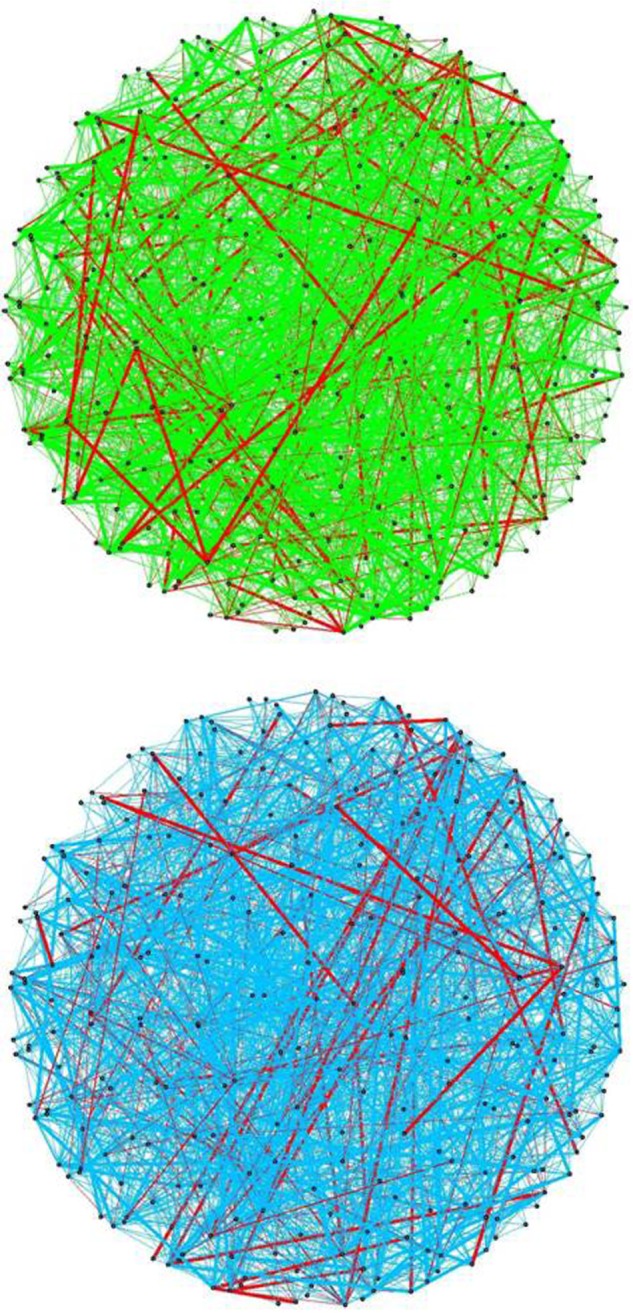
(A) Aggregated network for normal samples, (B) Aggregated network for tumor samples. Edges in red show those common among the estimates in (A) and (B).

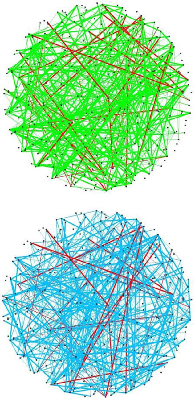
Figure 4.

Aggregated network, cutoff = |K|: (A) Aggregated network for normal samples, (B) Aggregated network for tumor samples. Edges in red show those common among the estimates in (A) and (B).

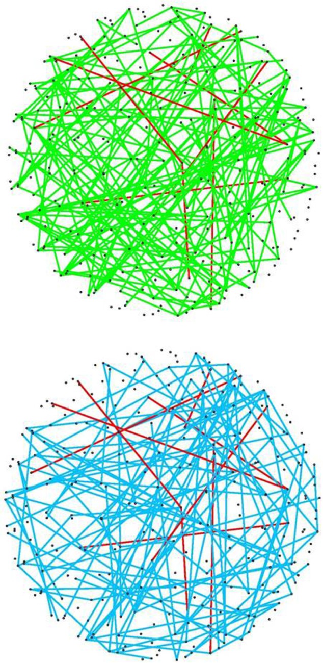
Figure 2 by itself does not provide useful information, as it shows the union of the edges estimated networks. To delineate the differences among normal and tumor networks, we can apply a cutoff τ to limit the edges of the network to those appearing in at least τ networks. In other words, for a given value of τ, we calculate a new adjacency matrix whose [i,j] element is zero if adj^Agg[i,j] < τ. Figure 3 shows the aggregated network with τ = 5. For this value of τ, the normal and tumor networks have 416 and 396, respectively, out of which only 37 appear in both network (red edges). This finding corroborates with our earlier observation that only a small fraction of edges estimated in normal and tumor networks are in common to both.

Figure 3.

Aggregated network, cutoff = 5: (A) Aggregated network for normal samples, (B) Aggregated network for tumor samples. Edges in red show those common among the estimates in (A) and (B).

Figure 4 shows the extreme case of looking at most consistent edges among estimated networks. In other words, the networks in Figure 4 are obtained by setting τ = |K| = 7, where K is the set of methods considered. The networks of normal and tumor samples have 174 and 133 edges, respectively. Similar to the previous settings, only nine edges are in common between the two networks, indicating a small amount of agreement between the networks estimated from two different conditions.

Tables S12 and S13 and Figures S4–S9 in Supplementary material compare the aggregated networks of normal and tumor samples normalized using two other preprocessing methods. The results show that similar patterns of differences among normal and tumor samples are observed, regardless of how the data are preprocessed.

Discussion

Gene networks provide useful information about interactions among genes, as well as new insight into complex biological systems. Increasing evidence also suggests an association between alterations in genetic networks and initiation and progression of complex diseases. However, existing repositories of biological networks only include information about genetic interactions in a single condition, often the “normal” or laboratory state of the cell. Therefore, these public repositories do not offer insight into changes in biological networks associated with complex diseases. Computational methods for network reconstruction are hence critical for understanding alterations in biological networks.

In this paper, we conducted an extensive empirical study to compare seven network reconstruction methods, by examining the differences in their estimated networks. We also investigated differences in networks corresponding to genetic interactions in normal versus tumor samples. The results suggest that

1. the degree distributions of networks obtained from different reconstruction methods have a considerable amount of heterogeneity;

2. there is a considerable amount of stochasticity or randomness in networks using computational methods; and

3. significant differences exist among networks of normal and tumor samples.

More research is thus needed to make network reconstruction methods a useful tool for studying changes in biological networks associated with complex diseases. First, current research often focuses on accuracy of reconstruction methods in terms of edge discovery (using eg, true positive and false positive rates or precision and recall). However, little has been done to understand other properties of networks constructed using computational methods, including local (degree distribution, etc.) and global (conductance, diameter, etc.) network properties. Second, despite significant progress in development of network reconstruction methods, characterization of the uncertainty of the estimated edges has not received much attention in the literature, and more research is needed in this area. Finally, a lot more research is needed to understand the differences among networks estimated under different disease or experimental conditions. Such research will offer the opportunity to systematically test for differential network structures and their associations with complex diseases.

Supplementary Data

Table S1. The list of data sets used in this study.

Table S2. The number of edges in estimated networks for normal and tumor samples, as well as the number of common edges between them.

Table S3. The number of edges in aggregated networks for normal and tumor samples and the number of common edges between them at different cutoff values.

Tables S4 and S5. The number of edges in estimated networks of normal and tumor samples by different methods as well as the corresponding tuning parameters.

Tables S6–S11. Similar to Tables 1 and 2, these show selected properties of estimated networks with 800, 900, and 1000 edges for normal and tumor samples.

Tables S12 and S13. Results of comparing the number of edges common to normal and tumor samples in original and permuted samples normalized using two other normalization methods, namely, normalize-then-merge and merge-then-normalize.

Figure S1. Data pre-processing using normalize-then-merge technique.

Figure S2. Data pre-processing using merge-then-normalize technique.

Figure S3. Data pre-processing using COMBAT.

Figure S4. Aggregated networks of (a) normal and (b) tumor samples preprocessed using normalize-then-merge method. An edge is included if it appears in at least τ = 1 estimated networks. Edges in red show those common among the estimates in (a) and (b).

Figure S5. Aggregated networks of (a) normal and (b) tumor samples preprocessed using normalize-then-merge method. An edge is included if it appears in at least τ = 5 estimated networks. Edges in red show those common among the estimates in (a) and (b).

Figure S6. Aggregated networks of (a) normal and (b) tumor samples preprocessed using normalize-then-merge method. An edge is included if it appears in at least τ = |K| = 7 estimated networks. Edges in red show those common among the estimates in (a) and (b).

Figure S7. Aggregated networks of (a) normal and (b) tumor samples preprocessed using merge-then-normalize method. An edge is included if it appears in at least τ = 1 estimated networks. Edges in red show those common among the estimates in (a) and (b).

Figure S8. Aggregated networks of (a) normal and (b) tumor samples preprocessed using merge-then-normalize method. An edge is included if it appears in at least τ = 5 estimated networks. Edges in red show those common among the estimates in (a) and (b).

Figure S9. Aggregated networks of (a) normal and (b) tumor samples preprocessed using merge-then-normalize method. An edge is included if it appears in at least τ = |K| = 7 estimated networks. Edges in red show those common among the estimates in (a) and (b).

REFERENCES

- 1.Baitaluk M, Sedova M, Ray A, Gupta A. BiologicalNetworks: visualization and analysis tool for systems biology. Nucleic Acids Res. 2006;34(suppl 2):W466–71. doi: 10.1093/nar/gkl308. [DOI] [PMC free article] [PubMed] [Google Scholar]
- 2.Ourfali O, Shlomi T, Ideker T, Ruppin E, Sharan R. SPINE: a framework for signaling-regulatory pathway inference from cause-effect experiments. Bioinformatics. 2007;23(13):i359–66. doi: 10.1093/bioinformatics/btm170. [DOI] [PubMed] [Google Scholar]
- 3.Novershtern N, Regev A, Friedman N. Physical module networks: an integrative approach for reconstructing transcription regulation. Bioinformatics. 2011;27(13):i177–85. doi: 10.1093/bioinformatics/btr222. [DOI] [PMC free article] [PubMed] [Google Scholar]
- 4.Nepusz T, Yu H, Paccanaro A. Detecting overlapping protein complexes in protein-protein interaction networks. Nat Methods. 2012;9(5):471–2. doi: 10.1038/nmeth.1938. [DOI] [PMC free article] [PubMed] [Google Scholar]
- 5.Spirin V, Mirny LA. Protein complexes and functional modules in molecular networks. Proc Natl Acad Sci USA. 2003;100(21):12123–8. doi: 10.1073/pnas.2032324100. [DOI] [PMC free article] [PubMed] [Google Scholar]
- 6.Parsons AB, Brost RL, Ding H, et al. Integration of chemical-genetic and genetic interaction data links bioactive compounds to cellular target pathways. Nat Biotechnol. 2004;22(1):62–9. doi: 10.1038/nbt919. [DOI] [PubMed] [Google Scholar]
- 7.Kelley R, Ideker T. Systematic interpretation of genetic interactions using protein networks. Nat Biotechnol. 2005;23(5):561–6. doi: 10.1038/nbt1096. [DOI] [PMC free article] [PubMed] [Google Scholar]
- 8.Ye P, Peyser BD, Pan X, Boeke JD, Spencer FA, Bader JS. Gene function prediction from congruent synthetic lethal interactions in yeast. Mol Syst Biol. 2005;1(1) doi: 10.1038/msb4100034.. [DOI] [PMC free article] [PubMed] [Google Scholar]
- 9.Barutcuoglu Z, Schapire RE, Troyanskaya OG. Hierarchical multi-label prediction of gene function. Bioinformatics. 2006;22(7):830–6. doi: 10.1093/bioinformatics/btk048. [DOI] [PubMed] [Google Scholar]
- 10.Murali TM, Wu C-J, Kasif S. The art of gene function prediction. Nat Biotechnol. 2006;24(12):1474–5. doi: 10.1038/nbt1206-1474. [DOI] [PubMed] [Google Scholar]
- 11.Kitano H. Foundations of Systems Biology. Cambridge: MIT Press; 2001. [Google Scholar]
- 12.Edelman GM, Gally JA. Degeneracy and complexity in biological systems. Proc Natl Acad Sci USA. 2001;98(24):13763–8. doi: 10.1073/pnas.231499798. [DOI] [PMC free article] [PubMed] [Google Scholar]
- 13.Yousef M, Ketany M, Manevitz L, Showe LC, Showe MK. Classification and biomarker identification using gene network modules and support vector machines. BMC Bioinformatics. 2009;10(1):337. doi: 10.1186/1471-2105-10-337. [DOI] [PMC free article] [PubMed] [Google Scholar]
- 14.Chen L, Xuan J, Riggins RB, Clarke R, Wang Y. Identifying cancer biomarkers by network-constrained support vector machines. BMC Syst Biol. 2011;5(1):161. doi: 10.1186/1752-0509-5-161. [DOI] [PMC free article] [PubMed] [Google Scholar]
- 15.Rapaport F, Zinovyev A, Dutreix M, Barillot E, Vert JP. Classification of microarray data using gene networks. BMC Bioinformatics. 2007;8(1):35. doi: 10.1186/1471-2105-8-35. [DOI] [PMC free article] [PubMed] [Google Scholar]
- 16.Hu P, Bull SB, Jiang H. Gene network modular-based classification of microarray samples. BMC Bioinformatics. 2012;13(suppl 10):S17. doi: 10.1186/1471-2105-13-S10-S17. [DOI] [PMC free article] [PubMed] [Google Scholar]
- 17.Zhu Y, Shen X, Pan W. Network-based support vector machine for classification of microarray samples. BMC Bioinformatics. 2009;10(suppl 1):S21. doi: 10.1186/1471-2105-10-S1-S21. [DOI] [PMC free article] [PubMed] [Google Scholar]
- 18.Ross DT, Scherf U, Eisen MB, et al. Systematic variation in gene expression patterns in human cancer cell lines. Nat Genet. 2000;24(3):227–35. doi: 10.1038/73432. [DOI] [PubMed] [Google Scholar]
- 19.Hu JJ, Smith TR, Miller MS, Lohman K, Case LD. Genetic regulation of ionizing radiation sensitivity and breast cancer risk. Environ Mol Mutagen. 2002;39(2–3):208–15. doi: 10.1002/em.10058. [DOI] [PubMed] [Google Scholar]
- 20.De Craene B, Berx G. Regulatory networks defining EMT during cancer initiation and progression. Nat Rev Cancer. 2013;13(2):97–110. doi: 10.1038/nrc3447. [DOI] [PubMed] [Google Scholar]
- 21.Wu C, Zhu J, Zhang X. Network-based differential gene expression analysis suggests cell cycle related genes regulated by E2F1 underlie the molecular difference between smoker and non-smoker lung adenocarcinoma. BMC Bioinformatics. 2013;14(1):365. doi: 10.1186/1471-2105-14-365. [DOI] [PMC free article] [PubMed] [Google Scholar]
- 22.Gill R, Datta S, Datta S. Differential network analysis in human cancer research. Curr Pharm Des. 2014;20(1):4–10. doi: 10.2174/138161282001140113122316. [DOI] [PMC free article] [PubMed] [Google Scholar]
- 23.Gill R, Datta S, Datta S. A statistical framework for differential network analysis from microarray data. BMC Bioinformatics. 2010;11(1):95. doi: 10.1186/1471-2105-11-95. [DOI] [PMC free article] [PubMed] [Google Scholar]
- 24.Chatr-Aryamontri A, Breitkreutz BJ, Heinicke S, et al. The BioGRID interaction database: 2013 update. Nucleic Acids Res. 2013;41(D1):D816–23. doi: 10.1093/nar/gks1158. [DOI] [PMC free article] [PubMed] [Google Scholar]
- 25.Prasad TSK, Goel R, Kandasamy K, et al. Human protein reference database-2009 update. Nucleic Acids Res. 2009;37(suppl 1):D767–72. doi: 10.1093/nar/gkn892. [DOI] [PMC free article] [PubMed] [Google Scholar]
- 26.Aranda B, Achuthan P, Alam-Faruque Y, et al. The IntAct molecular interaction database in 2010. Nucleic Acids Res. 2010;38(suppl 1):D525–31. doi: 10.1093/nar/gkp878. [DOI] [PMC free article] [PubMed] [Google Scholar]
- 27.Xenarios I, Salwinski L, Duan XJ, Higney P, Kim S-M, Eisenberg D. DIP, the database of interacting proteins: a research tool for studying cellular networks of protein interactions. Nucleic Acids Res. 2002;30(1):303–5. doi: 10.1093/nar/30.1.303. [DOI] [PMC free article] [PubMed] [Google Scholar]
- 28.Xenarios I, Rice DW, Salwinski L, Baron MK, Marcotte EM, Eisenberg D. DIP: the database of interacting proteins. Nucleic Acids Res. 2000;28(1):289–91. doi: 10.1093/nar/28.1.289. [DOI] [PMC free article] [PubMed] [Google Scholar]
- 29.Warde-Farley D, Donaldson SL, Comes O, et al. The GeneMANIA prediction server: biological network integration for gene prioritization and predicting gene function. Nucleic Acids Res. 2010;38(suppl 2):W214–20. doi: 10.1093/nar/gkq537. [DOI] [PMC free article] [PubMed] [Google Scholar]
- 30.Beyer A, Bandyopadhyay S, Ideker T. Integrating physical and genetic maps: from genomes to interaction networks. Nat Rev Genet. 2007;8(9):699–710. doi: 10.1038/nrg2144. [DOI] [PMC free article] [PubMed] [Google Scholar]
- 31.Shojaie A, Jauhiainen A, Kallitsis M, Michailidis G. Inferring regulatory networks by combining perturbation screens and steady state gene expression profiles. PLoS One. 2014;9(2):e82393. doi: 10.1371/journal.pone.0082393. [DOI] [PMC free article] [PubMed] [Google Scholar]
- 32.Edgar R, Domrachev M, Lash AE. Gene Expression Omnibus: NCBI gene expression and hybridization array data repository. Nucleic Acids Res. 2002;30(1):207–10. doi: 10.1093/nar/30.1.207. [DOI] [PMC free article] [PubMed] [Google Scholar]
- 33.Kanehisa M, Goto S. KEGG: Kyoto encyclopedia of genes and genomes. Nucleic Acids Res. 2000;28(1):27–30. doi: 10.1093/nar/28.1.27. [DOI] [PMC free article] [PubMed] [Google Scholar]
- 34.Irizarry RA, Bolstad BM, Collin F, Cope LM, Hobbs B, Speed TP. Summaries of Affymetrix GeneChip probe level data. Nucleic Acids Res. 2003;31(4):e15. doi: 10.1093/nar/gng015. [DOI] [PMC free article] [PubMed] [Google Scholar]
- 35.Johnson WE, Li C, Rabinovic A. Adjusting batch effects in microarray expression data using empirical Bayes methods. Biostatistics. 2007;8(1):118–27. doi: 10.1093/biostatistics/kxj037. [DOI] [PubMed] [Google Scholar]
- 36.Taminau Jonatan, Meganck Stijn, Lazar Cosmin, Steenhoff David, Coletta Alain, Molter Colin, Duque Robin, et al. Unlocking the potential of publicly available microarray data using inSilicoDb and inSilicoMerging R/Bioconductor packages. BMC bioinformatics. 2012;13(1):335. doi: 10.1186/1471-2105-13-335. [DOI] [PMC free article] [PubMed] [Google Scholar]
- 37.Bickel DR. Probabilities of spurious connections in gene networks: application to expression time series. Bioinformatics. 2005;21(7):1121–8. doi: 10.1093/bioinformatics/bti140. [DOI] [PubMed] [Google Scholar]
- 38.Kostka D, Spang R. Finding disease specific alterations in the co-expression of genes. Bioinformatics. 2004;20(suppl 1):i194–9. doi: 10.1093/bioinformatics/bth909. [DOI] [PubMed] [Google Scholar]
- 39.Stuart JM, Segal E, Koller D, Kim SK. A gene-coexpression network for global discovery of conserved genetic modules. Science. 2003;302(5643):249–55. doi: 10.1126/science.1087447. [DOI] [PubMed] [Google Scholar]
- 40.Smith VA, Jarvis ED, Hartemink AJ. Evaluating functional network inference using simulations of complex biological systems. Bioinformatics. 2002;18(suppl 1):S216–24. doi: 10.1093/bioinformatics/18.suppl_1.s216. [DOI] [PubMed] [Google Scholar]
- 41.Schäfer J, Strimmer K. An empirical Bayes approach to inferring large-scale gene association networks. Bioinformatics. 2005;21(6):754–764. doi: 10.1093/bioinformatics/bti062. [DOI] [PubMed] [Google Scholar]
- 42.Voorman A, Shojaie A, Witten D. Graph estimation with joint additive models. Biometrika. 2012;99(1):1–25. doi: 10.1093/biomet/ast053. [DOI] [PMC free article] [PubMed] [Google Scholar]
- 43.Zhao T, Liu H, Roeder K, Lafferty J, Wasserman L. The huge package for high-dimensional undirected graph estimation in R. J Mach Learn Res. 2012;13(1):1059–62. [PMC free article] [PubMed] [Google Scholar]
- 44.Margolin AA, Nemenman I, Basso K, et al. ARACNE: an algorithm for the reconstruction of gene regulatory networks in a mammalian cellular context. BMC Bioinformatics. 2006;7(suppl 1):S7. doi: 10.1186/1471-2105-7-S1-S7. [DOI] [PMC free article] [PubMed] [Google Scholar]
- 45.Langfelder P, Horvath S. WGCNA: an R package for weighted correlation network analysis. BMC Bioinformatics. 2008;9(1):559. doi: 10.1186/1471-2105-9-559. [DOI] [PMC free article] [PubMed] [Google Scholar]
- 46.Friedman J, Hastie T, Tibshirani R. Sparse inverse covariance estimation with the graphical lasso. Biostatistics. 2008;9(3):432–41. doi: 10.1093/biostatistics/kxm045. [DOI] [PMC free article] [PubMed] [Google Scholar]
- 47.Meinshausen N, BuHlmann P. High-dimensional graphs and variable selection with the lasso. Ann Stat. 2006;34(3):1436–62. [Google Scholar]
- 48.Fan J, Feng Y, Wu Y. Network exploration via the adaptive LASSO and SCAD penalties. Ann Appl Stat. 2009;3(2):521. doi: 10.1214/08-AOAS215SUPP. [DOI] [PMC free article] [PubMed] [Google Scholar]
- 49.Shimamura T, Imoto S, Yamaguchi R, Miyano S. Weighted lasso in graphical Gaussian modeling for large gene network estimation based on microarray data. Genome Inform. 2007;19:142–53. [PubMed] [Google Scholar]
- 50.Danaher P, Wang P, Witten DM. The joint graphical lasso for inverse covariance estimation across multiple classes. J R Stat Soc Series B Stat Methodol. 2013 doi: 10.1111/rssb.12033. [DOI] [PMC free article] [PubMed] [Google Scholar]
- 51.Peng J, Wang P, Zhou N, Zhu J. Partial correlation estimation by joint sparse regression models. J Am Stat Assoc. 2009;104(486):735–46. doi: 10.1198/jasa.2009.0126. [DOI] [PMC free article] [PubMed] [Google Scholar]
- 52.Li A, Horvath S. Network neighborhood analysis with the multi-node topological overlap measure. Bioinformatics. 2007;23(2):222–31. doi: 10.1093/bioinformatics/btl581. [DOI] [PubMed] [Google Scholar]
- 53.Yip AM, Horvath S. Gene network interconnectedness and the generalized topological overlap measure. BMC Bioinformatics. 2007;8(1):22. doi: 10.1186/1471-2105-8-22. [DOI] [PMC free article] [PubMed] [Google Scholar]
- 54.Meyer PE, Lafitte F, Bontempi G. minet: a R/Bioconductor package for inferring large transcriptional networks using mutual information. BMC Bioinformatics. 2008;9(1):461. doi: 10.1186/1471-2105-9-461. [DOI] [PMC free article] [PubMed] [Google Scholar]
- 55.Shojaie A, Basu S, Michailidis G. Adaptive thresholding for reconstructing regulatory networks from time-course gene expression data. Stat Biosci. 2012;4(1):66–83. [Google Scholar]
- 56.Jacob L, Obozinski G, Vert JP. Group lasso with overlap and graph lasso; Paper presented at: Proceedings of the 26th Annual International Conference on Machine Learning; 2009; Montreal, Canada. [Google Scholar]
- 57.Meier L, Van De Geer S, Bühlmann P. The group lasso for logistic regression. J R Stat Soc Series B Stat Methodol. 2008;70(1):53–71. [Google Scholar]
Associated Data
This section collects any data citations, data availability statements, or supplementary materials included in this article.
Supplementary Materials