On the definition and utilization of heritable variation among hosts in reproduction ratio R₀ for infectious diseases

Abstract

Infectious diseases have a major role in evolution by natural selection and pose a worldwide concern in livestock. Understanding quantitative genetics of infectious diseases, therefore, is essential both for understanding the consequences of natural selection and for designing artificial selection schemes in agriculture. The basic reproduction ratio, R₀, is the key parameter determining risk and severity of infectious diseases. Genetic improvement for control of infectious diseases in host populations should therefore aim at reducing R₀. This requires definitions of breeding value and heritable variation for R₀, and understanding of mechanisms determining response to selection. This is challenging, as R₀ is an emergent trait arising from interactions among individuals in the population. Here we show how to define breeding value and heritable variation for R₀ for genetically heterogeneous host populations. Furthermore, we identify mechanisms determining utilization of heritable variation for R₀. Using indirect genetic effects, next-generation matrices and a SIR (Susceptible, Infected and Recovered) model, we show that an individual's breeding value for R₀ is a function of its own allele frequencies for susceptibility and infectivity and of population average susceptibility and infectivity. When interacting individuals are unrelated, selection for individual disease status captures heritable variation in susceptibility only, yielding limited response in R₀. With related individuals, however, there is a secondary selection process, which also captures heritable variation in infectivity and additional variation in susceptibility, yielding substantially greater response. This shows that genetic variation in susceptibility represents an indirect genetic effect. As a consequence, response in R₀ increased substantially when interacting individuals were genetically related.

Introduction

Infectious diseases are widespread in humans, animals and plants. In natural populations, infectious diseases have a major role in the process of evolution by natural selection (Haldane, 1949; O'Brien and Evermann, 1988). In domestic populations, particularly in livestock, infectious diseases are imposing a worldwide concern owing to their impact on the welfare and productivity of livestock, and in the case of zoonosis, also because of the threat for human health. To contain the threat imposed by infectious diseases, different control strategies such as vaccination, antibiotic treatments and management practices have been implemented widely. However, the evolution of resistance to antibiotics by bacteria, evolution of resistance to vaccines by viruses and undesirable environmental impacts of antibiotic treatment put these strategies under question (Gibson and Bishop, 2005). Thus, there is a need to investigate additional control strategies, so as to extend the repertoire of possible interventions. A greater repertoire is favourable (1) because it allows for a change in approach when certain control measures fail and (2) because the use of combinations of control measures make emergence of resistance against control more difficult.

Several studies have demonstrated the existence of genetic variation for different disease traits for a wide variety of infectious diseases. Examples are clinical mastitis and Mycobacterium bovis infections in dairy cattle (Heringstad et al., 2005). Such studies usually focus on estimating the genetic variance in individual disease status. As this approach connects an individual's own disease status to its own pedigree, it only captures heritable variation in susceptibility (or resistance) to disease (Lipschutz-Powell et al., 2012). However, host genetic variation may be present also in other traits that affect the dynamics of infectious diseases in populations. Thus, to use a general term for such other traits, infectivity will also have an impact on the transmission of infectious diseases. There clearly exists (phenotypic) variation in infectivity as it can be seen from the occurrence of superspreaders (Lloyd-Smith et al., 2005). Thus, it is most likely that the classical quantitative genetic analysis based on individual disease status captures only part of the possible heritable variation in the host underlying infectious disease dynamics (Lipschutz-Powell et al., 2012).

The ultimate goal of selective breeding for disease traits is to reduce the risk of an epidemic and/or to reduce the level of the endemic equilibrium. In epidemiology, the key parameter determining the risk and size of an epidemic and/or the level of the endemic equilibrium is the basic reproduction ratio, R₀. R₀ is the average number of secondary cases produced by a typical infectious individual during its entire infectious life time, in an otherwise naive population (Diekmann et al., 1990). R₀ has a threshold value of 1, which determines whether a major disease outbreak can occur or whether the endemic equilibrium exists. When R₀<1, the epidemic will die out. On the other hand, when R₀>1 major outbreaks or an endemic equilibrium (persistence) can occur. Hence, breeding strategies to reduce the risk and prevalence of an infectious disease should aim at reducing R₀, preferably to below a value of 1.

Breeding to reduce R₀ raises a conceptual difference between quantitative genetics and epidemiology: R₀ is an epidemiological parameter referring to an entire population, whereas quantitative genetics rests on the concept of breeding value, which refers to a single individual. It is clear that in a genetically heterogeneous population, R₀ is a function of individual genotypes in the population, which in turn are a function of allele frequencies. Moreover, a change in allele frequencies will change R₀, indicating R₀ can respond to selection. Genetic improvement aiming to reduce R₀ should ideally be based on the effects of an individual's genes on R₀, which would require defining individual breeding values for R₀. Moreover, defining a breeding value for R₀ would also allow defining heritable variation in R₀, that is, the variation in individual breeding values for R₀, which would give an indication of the prospects for genetic improvement with respect to R₀.

For domestic populations, the subsequent question would be how to design breeding programs, so as to utilize optimally heritable variation in R₀ and achieve the greatest possible rate of reduction in R₀. The equivalent issue for natural populations would be what ecological conditions are favourable for efficient reduction of R₀ by natural selection. For emergent traits that depend on multiple individuals, research in the field of indirect genetic effects (IGEs) suggests that group selection and relatedness among interacting individuals (‘kin selection') can be used to increase response to selection (Griffing, 1976; Bijma, 2011). This suggests that relatedness and group selection may be important mechanisms affecting the utilization of heritable variation in R₀, either by natural or artificial selection.

Here we show how to define breeding value and heritable variation for R₀ for a genetically heterogeneous host population, where individuals differ for susceptibility and infectivity. For that purpose, we have adapted the theory of IGEs commonly applied to socially affected traits, using the epidemiological concept of next-generation matrices (NGMs) (Diekmann et al., 1990, 2010). Furthermore, we examine the mechanisms determining the utilization of heritable variation in R₀, focusing on the effects of kin selection on response in R₀, and in susceptibility and infectivity.

Materials and methods

Dynamic model of infection

In a completely naive population where a microparasitic infection is introduced, the disease dynamics can be modelled with a basic compartmental stochastic SIR (Susceptible, Infected and Recovered) model. In this model, individuals move through the states in the order S→I→R (Anderson et al., 1992). Therefore, the possible events that an individual may encounter are infection and recovery. With stochasticity, these events occur randomly at a certain rate (probability per unit of time) specified by the model parameters. In the SIR model, these parameters are the transmission rate parameter (β) for S→I, and the recovery rate parameter (α) for I→R. The transmission rate parameter β is the probability per unit of time that a typical infected individual infects another individual in a totally susceptible population (Diekmann et al., 1990; Anderson et al., 1992). When constant population density is assumed, the rate at which the susceptible population becomes infected is βSI/N, where S denotes the number of susceptible individuals, I the number of infectious individuals and N the total number of individuals in the population (Kermack and McKendrick, 1991). The recovery rate parameter α is the probability per unit of time for an infective to recover from an infection. In other words, for constant α, the infectious period is exponentially distributed with a mean duration of α⁻¹ time units.

The transmission rate parameter, β, depends on the infectivity of infectious individuals and on the susceptibility of uninfected recipient individuals. Thus, in a homogeneous population where all individuals have the same level of infectivity and susceptibility, there is a single β that applies to the whole population, which can be defined as a function of these parameters,

where γ is susceptibility, ϕ is infectivity and c is average number of contacts an infectious individual makes per unit of time (see Table 1 for a notation key).

Table 1. Notation key.

Symbol	Meaning
γG	Effect of G allele at susceptibility locus
γg	Effect of g allele at susceptibility locus
ϕF	Effect of F allele at infectivity locus
ϕf	Effect of f allele at infectivity locus
pg	Frequency of the g allele for susceptibility
pf	Frequency of the f allele for infectivity
	Average individual susceptibility
	Average individual infectivity
rγ	Relatedness at susceptibility locus
rϕ	Relatedness at infectivity locus
βij	Pairwise transmission rate parameter between susceptible individual i and infective individual j
α	Rate of recovery parameter
c	Contact rate
R0	Basic reproduction ratio
	Breeding value for R0 of individual i
	Additive standard deviation in total breeding value
D	Measure of linkage disequilibrium
FIS	Measure of deviation from Hardy–Weinberg equilibrium

Dynamic model of infection with genetic heterogeneity

In a genetically heterogeneous population, however, the transmission rate parameter β may vary among pairs of individuals. This pairwise transmission rate will depend on the infectivity genotype of the infectious individual and on the susceptibility genotype of the recipient susceptible individual. The assumption that transmission depends on the infectivity of only the infectious individual and on the susceptibility of only the recipient individual is known as separable mixing (Diekmann et al., 1990). Thus, we may define the pairwise transmission rate parameter β_ij from an infectious individual j to a susceptible individual i as

where γ_i denotes susceptibility of susceptible individual i and ϕ_j denotes infectivity of infectious individual j. In Equation (2), c represents the average contact rate; any variation in contact rate among susceptible and infectious individuals is included in γ_i and ϕ_i because of the assumption of separable mixing.

In the following, we model genetic heterogeneity in a diploid population using two biallelic loci, one locus for susceptibility effect (γ) and the other locus for infectivity effect (ϕ). The susceptibility locus has alleles G and g, with susceptibility values γ_G and γ_g, respectively, and the infectivity locus has alleles F and f, with infectivity values ϕ_F and ϕ_f, respectively. Furthermore, both loci are assumed to have additive allelic effects without dominance. Thus, genotypic values are given by γ_GG=γ_G+γ_G=2γ_G, γ_gg=γ_g+γ_g=2γ_g and γ_Gg=γ_gG=γ_G+γ_g for susceptibility, and ϕ_FF=ϕ_F+ϕ_F=2ϕ_F, ϕ_ff=ϕ_f+ϕ_f=2ϕ_f and ϕ_Ff=ϕ_fF=ϕ_F+ϕ_f for infectivity. As we assumed additive gene action, average susceptibility in the population is given by

and average infectivity is given by

where p_f is the frequency of the f allele, p_g the frequency of the g allele and the ‘2' arises because each individual carries two alleles. Note that and are average susceptibility and average infectivity over individuals, and not average of allele effects. In a population as defined here, there are nine genotypes of individuals because of the combinations of their genotype for susceptibility and infectivity.

For this heterogeneous population, we can now construct the NGM. The NGM describes the number of infectious individual of each type in the next generation of the epidemic, produced by infectious individuals of each type in the current generation. Then, we can calculate R₀ as the dominant eigenvalue of the NGM. Under the assumption of separable mixing, the dominant eigenvalue equals the trace of a matrix, and thus R₀ can be obtained as the trace of the NGM (Diekmann et al., 2010).

Appendix 1 shows the NGM for the population with linkage equilibrium and in Hardy–Weinberg Equilibrium (HWE) described by Equations (2), (3), (4). R₀ is given by the trace of the NGM:

where α is the recovery rate, which is assumed to be the same for all individuals in the population.

The NGM was also constructed for the more general case of a population that deviates from HWE and linkage equilibrium. For that case, R₀ is given by (Appendix 2)

where F_IS is the inbreeding coefficient and measures deviation of the population from HWE. It is a function of observed heterozygosity (H_o) and expected heterozygosity (H_e) in the population,

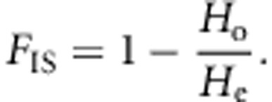The D measures the deviation of the population from linkage equilibrium and expresses the excess of coupling phase haplotypes (Falconer and Mackay, 1996),

The second term in brackets in Equation (6) is the covariance between susceptibility and infectivity of individuals in the population. When either (i) D=0 or (ii) F_IS=−1, that is, full disassortative ordering of alleles over diploid organisms (H_o=2H_e=1, which requires p=1/2) or (iii) there is no variance in either of the two traits ( or ), then there is no covariance between the two traits and R₀ is given by Equation (5).

Individual breeding value for R₀

Equation (5) gives R₀, which is an emergent trait of the population, that is, a trait that arises when the different individuals (susceptible and infectious) interact (Dawkins, 2006). The objective here, however, is to define individual breeding values for R₀. We use results from the field of IGEs to define breeding value for R₀. An IGE is heritable effect of an individual on the trait value of another individual (Griffing, 1967, 1976, 1981; Moore et al., 1997; Wolf et al., 1998; Muir, 2005). Hence, infectivity is an IGE, as an individual's infectivity affects the disease status of its contacts. Moore et al. (1997) and Bijma et al. (2007) show how breeding value and genetic variance can be defined for such traits. Bijma (2011) shows how the approach can be generalized to any trait, including traits that are an emerging property of a population, such as R₀. They propose a (total) breeding value that follows from the genetic mean of the population, rather than from individual trait values.

In classical quantitative genetics, breeding value is the sum of the average effects of an individual's alleles on its trait value, where the average effects equal the partial regression coefficients of individual trait values on individual allele count (Fisher, 1919; Lynch and Walsh, 1998). For traits affected by IGEs, the total breeding value is the sum of the average effects of an individual's alleles on the mean trait value of the population (Bijma, 2011). For an emergent trait, however, there is only a single trait value for the entire population, and the average effects of alleles on that trait follow from the partial derivatives of the trait value with respect to allele frequency, rather than from partial regression of individual trait values on allele count. This is analogous to the derivation of economic values in livestock genetic improvement. Applying this approach to R₀ (Equation (5)) with linkage equilibrium and HWE, average effect of the g allele equals

and the average effect of the f allele on R₀ equals

Consequently, the individual breeding value for R₀ is given by

where p_g,i and p_f,i refer to the allele frequencies in individual i, thus taking values of 0, 1/2 or 1. The equation for for the population that deviates from HWE and with linkage disequilibrium (LD) is presented in Appendix 2.

In the following, we will refer to as the breeding value for R₀ of individual i. Note that, in contrast to the pairwise transmission rate parameter β_ij, an individual's breeding value for R₀ is entirely a function of its own genes. This is because an individual transmits its own genes to its offspring, which may differ from the genes affecting its own disease phenotype.

The relationship between the breeding values of the individuals in a population of n individuals and R₀ of that population is

The first term in Equation (8) is the intercept that determines the magnitude of R₀, but it does not depend on the allele frequencies and is not needed in the breeding value. The last term is there because of the nonlinear relationship between R₀ (Equation (5)) and susceptibility and infectivity. From Equation (8), it can be seen that changes in breeding value for R₀ will lead to corresponding changes (in magnitude and direction) in R₀ itself. Only when also the frequencies in whole populations (p_g, p_f) are changing, the change in R₀ will be more than the change in breeding values due to this last term. In that case, selection that reduces both susceptibility and infectivity will lead to a greater reduction in R₀ than predicted by the breeding values. Response to selection in R₀ will equal the change in average individual breeding value for R₀,

Hence, a (small) change in average individual breeding value for R₀ due to selection will generate the same change in R₀. Thus, just as with an ordinary breeding value (Fisher, 1919; Lynch and Walsh, 1998), for a small change in allele frequency, the change in mean breeding value for R₀ equals response to selection in R₀.

Heritable variation in R₀

Response to selection in any trait, including emergent traits such as R₀, can be expressed as the product of intensity of selection ι, accuracy of selection ρ_T and total genetic standard deviation for that trait (Bijma, 2011),

In the above equation, response to selection R is change in mean trait value from one generation to the next. The selection intensity ι is the selection differential expressed in standard deviation units. Accuracy of selection ρ_T is the correlation between the total breeding value and the selection criterion in the candidates for selection, and is the standard deviation in total breeding value for the trait in the candidates for selection. Selection intensity and accuracy of selection are scale-free parameters and do not include any information about the heritable variance in the trait. Standard deviation in total breeding value, on the other hand, reflects the potential of the population to response to selection. Note that heritable variation in the context of Equation (10) strictly refers to the potential of a population to respond to selection, and may differ from the classical additive genetic variance in a trait. R₀, for example, has no classical additive genetic variance, as there exist no individual phenotypes for R₀. Thus, in the following, heritable variation in R₀ will refer to the potential for genetic change in R₀, and not to the additive genetic component of phenotypic variation in R₀ among individuals. This conceptual difference is discussed in detail in Bijma (2011).

From the above, it follows that heritable variation in R₀ equals the variance in breeding value for R₀ among individuals in the population. We drop the prefix ‘total' from breeding value and heritable variation, as R₀ has no classical breeding value. Taking the variance of Equation (7c), assuming linkage equilibrium, shows that heritable variation in R₀ equals

where is the variance among individuals in breeding value for R₀. Hence, Equation (11) shows how heritable variation in R₀ depends on the susceptibility and infectivity effects of alleles and on the allele frequencies in the population.

The expression in Equation (11) may be recognized as the sum of the additive genetic variances at two independent loci. Additive genetic variance at a single locus is traditionally written as 2p(1−p)α², where α denotes the average effect of an allele substitution (Falconer and Mackay, 1996). In Equation (11), the average effect at the susceptibility locus equals 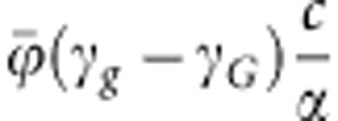, and average effect at the infectivity locus equals 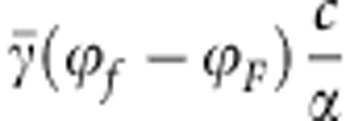(see also Equations (7a–c)).

Utilization of heritable variation in R₀

Efficient reduction of R₀ by means of selective breeding requires selection schemes that optimally utilize the heritable variation in R₀. Because an individual's infectivity represents an IGE, that is, a heritable effect of the individual on the disease status of other individuals within the same epidemiological unit, optimal breeding schemes for traits affected by IGEs may provide a clue for the design of optimal schemes for reducing R₀. For traits affected by IGEs, group selection and relatedness among interacting individuals (‘kin selection') increase response to selection (Griffing, 1967, 1976; Bijma and Wade, 2008). Moreover, Bijma (2011) shows that relatedness among interacting individuals in general tends to increase response to selection for traits that have an IGE. We, therefore, considered a group-structured population, where group mates can be genetically related. The objective of this section is not to precisely quantify or predict response to selection, but to identify and illustrate important factors affecting it.

To investigate mechanisms affecting response in R₀, a simulation study was performed on a population with discrete generations. The genetic model was the same as described above. The population was subdivided into 100 groups of 100 individuals each. In each group, an epidemic was started by a single randomly infected individual. After the end of an epidemic, selection was based on individual disease status (0/1), where only those that escaped the infection were selected from each group to be parent of the next generation. For the next generation, selected parents were mated randomly and offspring genotypes were randomly sampled based on the parental genotypes. The size and the number of groups were kept constant throughout the generations.

Each group in the population was set up in such a way that group mates showed a certain degree of genetic similarity, which we refer to as ‘relatedness', r, here. The term ‘relatedness' has different meanings in different scientific disciplines. In animal breeding, for example, relatedness is implicitly understood as ‘pedigree relatedness'. In sociobiology, such as in studies on the evolution of altruism, on the other hand, relatedness is interpreted as a more general measure of genetic similarity, irrespective of the cause of that similarity, for example, as a genetic regression coefficient (Hamilton, 1970; see also Frank, 1998). Here we define relatedness as the correlation between the allele count of group mates, irrespective of the cause of that correlation. This definition agrees with the use of relatedness in animal breeding applications, such as selection index theory and genomic relationship matrices, where the current population is treated as the base population (Falconer and Mackay, 1996).

Relatedness at the susceptibility locus, r_γ, and at the infectivity locus, r_ϕ, were allowed to differ. To achieve a certain relatedness among group mates, a fraction f of fully related individuals was added to each group, supplemented by a fraction 1−f of randomly selected individuals. We did not consider negative values for relatedness, because the lower bound for relatedness is practically zero when group size equals 100 individuals (r_min=−1/99). Appendix 3 shows that the required fraction equals the square root of relatedness. Thus, a fraction of individuals that were fully related to each other at the susceptibility locus, and a fraction of individuals that were fully related to each other at the infectivity locus were added to each group. As each individual carries both loci, these additions cannot be done independently; details of the strategy to jointly make those additions are given in Appendix 4.

The simulation was further extended to allow for a certain degree of LD between both loci. However, for a given LD in the population, there exists an upper and lower bound for r_γ given r_ϕ and vice versa. For example, when both loci are in strong positive LD and relatedness is zero at the susceptibility locus, then it is not possible to have very high relatedness at the infectivity locus. Appendix 5 provides expressions for those bounds.

Four different scenarios were simulated (Table 2). First, a scenario with heritable variation at both the susceptibility and the infectivity locus and groups created randomly with respect to relatedness r among group mates. No LD and a recombination rate θ of 0.5 between both loci were further assumed. Second, varying degrees of relatedness were used, which were the same at both loci. Third, to investigate a potential effect of relatedness on response in susceptibility, heritable variation was simulated at the susceptibility locus only, for varying degrees of relatedness among group mates. Finally, to investigate the potential effect of relatedness on response in R₀ in the case where there is strong negative LD between both loci and no recombination, a scenario with a relatedness of either 0 or 0.1 at both loci was simulated.

Table 2. Scenarios and parameter values.

Parameters	Scenario 1	Scenario 2	Scenario 3	Scenario 4
Allele effect at infectivity locus
ϕf	0.6	0.6	1	2.4
ϕF	1	1	1	0.6
Variation at
Susceptibility locus	Yes	Yes	Yes	Yes
Infectivity locus	Yes	Yes	No	Yes
Relatedness r	0	0–1	0–1	0 or 0.1
Linkage disequilibrium D	0	0	0	−0.20
Recombination rate θ	0.5	0.5	0.5	0

Note: Throughout the four scenarios, contact rate, c=2, recovery rate, α=0.5, and allele effect at susceptibility locus, γ_g=1 and γ_G=0.6, was used. Initial allele frequencies at both loci were set at 0.5. The r² statistic corresponding to D=−0.20 equals 0.64.

Simulation results

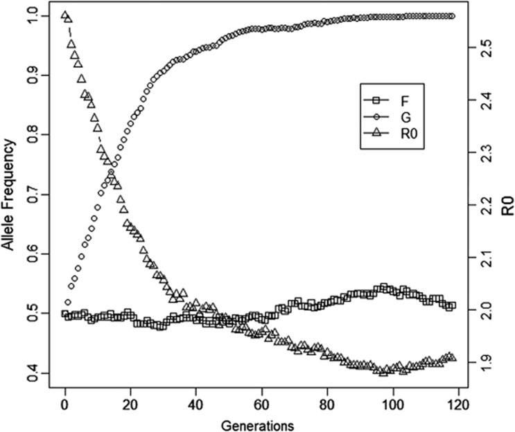
In the first scenario, which had unrelated group mates, a response to selection was observed only at the susceptibility locus, where the G allele became fixed after an average of 100 generations. At the infectivity locus, in contrast, only a random fluctuation of allele frequency was observed (Figure 1). Thus, with groups composed at random with respect to relatedness, no response was observed at the infectivity locus. As a result, in the final generation, the response in R₀ was limited.

Figure 1.

Allele frequency (F) at infectivity locus, allele frequency (G) at susceptibility locus and R₀ when there is no relatedness among group mates (Scenario 1, Table 2). Results are from one representative replicate.

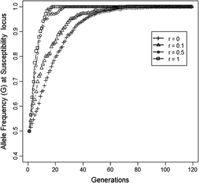
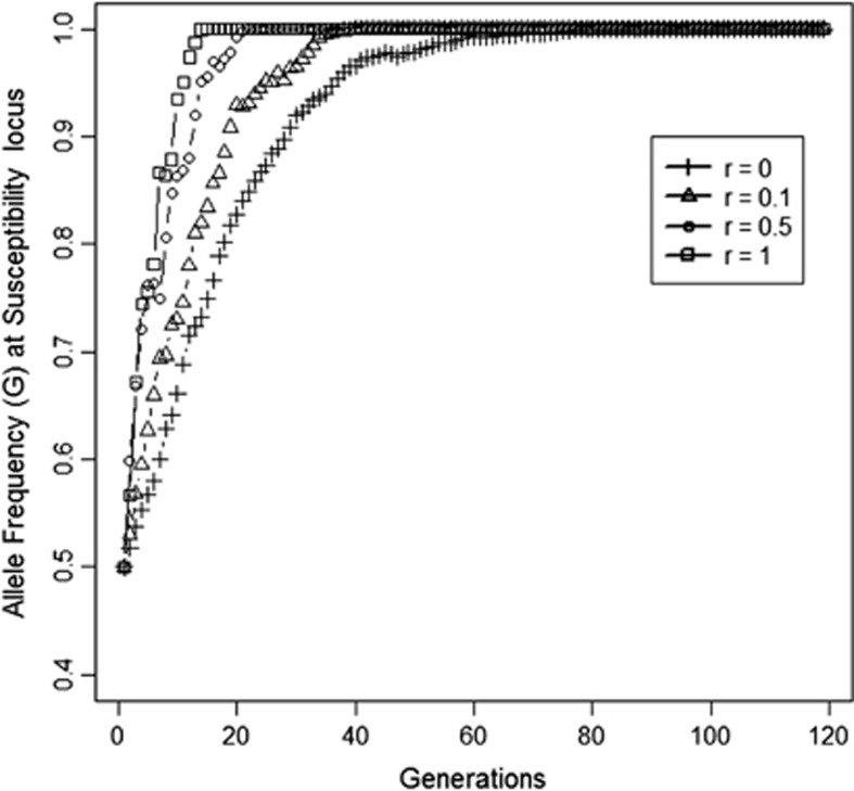
In the second scenario, which had related group mates, response to selection was observed at both loci, and the population became fixed for the G-allele at susceptibility locus and for F-the allele at the infectivity locus (Figures 2 and 3). In this case, selection resulted in a greater reduction of R₀ than in the first scenario (Figure 4 vs Figure 1). As relatedness among group mates increased, response was much faster in all three traits. As it was also faster on the susceptibility locus, this suggested that also the susceptibility locus showed an IGE.

Figure 2.

Allele frequency (F) at infectivity locus as relatedness among group mates increases from 0 to 1 (Scenario 2, Table 2). Results are from one representative replicate.

Figure 3.

Allele frequency (G) at susceptibility locus as relatedness among group mates increases from 0 to 1 (Scenario 2, Table 2). Results are from one representative replicate.

Figure 4.

R₀ when relatedness among group members increases from 0 to 1 (Scenario 2, Table 2). Results are from one representative replicate.

To verify this IGE in susceptibility in the third scenario, we chose to have variation in the susceptibility only. Also in this case, the response at the susceptibility locus increased substantially when relatedness among group mates increased (Figure 5). For selection on individual phenotype, it is known that relatedness increases response in the IGEs, but not in the direct genetic effects (Griffing, 1976; Bijma and Wade, 2008). Thus, this result suggests that (1) susceptibility not only has a direct genetic effect on the disease status of the individual itself but also has an IGE on the disease status of its groups mates, and that (2) this indirect genetic variance is utilized by kin selection (see Discussion), even in the absence of genetic variance in infectivity.

Figure 5.

Allele frequency (G) at susceptibility locus as relatedness increases from 0 to 1 in the population with heritable variation at susceptibility locus only (Scenario 3, Table 2). Results are from one representative replicate.

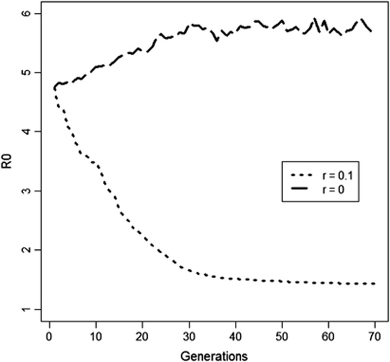
In the fourth scenario, which had strong negative LD and no recombination, the direction of response in R₀ depended on the relatedness among group mates. Without relatedness, selection fixed the G allele irrespective of the linked allele at the infectivity locus. As a consequence, selection increased the frequency of f allele, yielding an increase rather than a decrease of R₀. When relatedness r_γ=r_ϕ=0.1 was used, however, selection caused fixation of the GF haplotype, resulting in a decrease in R₀ (Figure 6). This result shows that kin selection can prevent a maladaptive response to selection.

Figure 6.

The effect of relatedness on response in mean R₀ in a population with strong negative LD (D=−0.20, →r²=0.64) and no recombination between susceptibility and infectivity locus. For ϕ_f=2.4 and ϕ_F=0.6. Initial R₀ was 4.7 (Scenarios 4a and b, Table 2). Results are from one representative replicate.

Discussion

The aim of this study was to define the breeding value and heritable variation for R₀. This was done for a diploid host population with genetic variation for susceptibility and infectivity. Breeding values of individuals were derived by finding the R₀, linearizing this value in the allele frequencies and substituting the individual's allele frequencies. The heritable variation that measures the potential for response in R₀ can then be found by taking the variance of the breeding values in the population. We applied this approach to a simple SIR model with genetic variation in susceptibility and infectivity, and assuming separable mixing.

The second focus of this paper was to investigate the mechanisms that affect response in R₀. As genetic relatedness between interacting individuals is expected to increase response in the general case (Bijma, 2011), we hypothesized that this result would extend to R₀ and considered a group-structured population with related group members. Our results show that, with unrelated group members and no LD between both loci, selection based on individual disease status yields response in susceptibility only. In the absence of relatedness, response in infectivity depends entirely on the correlation with susceptibility, which was zero in the absence of LD.

Relatedness among group members increased response in R₀ in two ways. First, with related group members, selection for individual disease status captures the heritable variation in infectivity. This occurs because an individual that carries the favourable allele for infectivity has group mates with a below-average infectivity, which increases its probability of escaping the epidemic, and thus being selected. Second, relatedness among group mates increases response in susceptibility. This occurs because an individual that carries the favourable allele for susceptibility on an average has fewer infected group mates, which increases its probability of escaping the epidemic and being selected. These results show that not only infectivity but also susceptibility exhibits an IGE; at the same level of infectivity, individuals with lower susceptibility have a reduced chance of infecting others simply because they have a lower chance of being infected themselves. The net result of both mechanisms is a strong increase in response to selection in R₀ when relatedness increases. To quantify the impact of relatedness on the accuracy of selection for R₀, we calculated the correlation between the selection criteria (healthy/infected) and the breeding value for R₀. Using the parameter values presented in Scenario 2, Table 2, accuracy of selection increased from 0.05 to 0.24 when relatedness increased from 0 to 1. Thus, our study further supports the claim of Bijma (2011) that relatedness is an important factor in utilization of heritable variation in traits affected by IGEs.

Our results suggest that relatedness among interacting individuals can be used in livestock breeding programs aiming to reduce disease incidence. In current breeding strategies in livestock, data on individual disease status is connected to the pedigree of individuals to estimate breeding values. When interacting individuals are unrelated, those breeding values capture only the direct genetic effect, that is, the direct genetic part of susceptibility. Breeding values can be improved by also considering IGEs, for example, by fitting direct–indirect genetic effects models to data on disease status (Lipschutz-Powell et al., 2012). However, estimating direct and indirect breeding values for disease status is methodologically challenging because the linear mixed models traditionally used in quantitative genetics do not fit the nonlinear dynamics of infectious diseases (Lipschutz-Powell et al., 2012). The use of related group members may offer a low-tech solution, for capturing more of the heritable variation in R₀ without the need to explicitly model IGEs.

In this work, we have assumed that the selection objective is to reduce R₀. While this is probably the obvious choice for epidemiologists, it may be unexpected for breeders who are not very familiar with R₀. For breeders, reducing disease incidence might be the more common objective. For example, in the context of our two-locus model, breeders might specify an objective H_i=v_γp_g,i+v_ϕp_f,i, where v_γ and v_ϕ are the so-called economic values for susceptibility and infectivity, respectively, which would be the partial derivatives of disease incidence with respect to the population allele frequencies p_g and p_f. However, both objectives are very similar, both for epidemic and endemic diseases. For epidemic diseases, the ultimately affected fraction of the population, known as the final size 1−s(∞), is determined by R₀, as is shown by the final size equation: ln s(∞)=R₀(s(∞)−1) (Kermack and McKendrick, 1991). For endemic diseases, the equilibrium-affected fraction is given by: 1−s(∞)=1−1/R₀. Hence, the relationship between disease incidence and allele frequency occurs entirely via R₀, both for epidemic and endemic diseases. Thus, when the objective is to decrease incidence, the economic values for any disease trait, say x, that is, the partial derivatives of incidence with respect to that trait, can be written as

In this expression, the ∂i/∂R₀ is a constant that is the same for all individuals in the population, and is independent of the disease trait considered (e.g. susceptibility or infectivity). Thus, the ranking of individuals will be the same, irrespective of whether they are ranked on breeding value for incidence or on breeding value for R₀.

Beware that breeding for incidence is not the same as breeding for susceptibility. When comparing breeding for susceptibility to breeding for R₀ or incidence, the latter is to be preferred because it also covers the heritable variation originating from infectivity (e.g. Figure 4 vs Figure 1).

With respect to the evolution of parasite virulence, also the key role of kin selection has been recognized (Levin and Pimentel, 1981; Frank, 1996; Galvani, 2003). Much less attention has been given to the potential for kin selection acting on the host population. Using Monte Carlo simulation, Fix (1984) showed that the presence of kin groups in a small-scale human population considerably accelerated the increase in frequency of a resistance allele. Schliekelman (2007) seems to be the first who used rigorous mathematical modelling to investigate the impact of kin selection on the frequency of mutant alleles conferring resistance to the host. Moreover, despite the evidence of heterogeneity in infectivity (Woolhouse et al., 1997; Lloyd-Smith et al., 2005; Doeschl-Wilson et al., 2011), little attention has been given to the effect of kin selection on the frequency of alleles affecting infectivity in the host population. Our simulations show that, at least in theory, kin selection can greatly accelerate the evolution of R₀, because it utilizes the indirect genetic variance in both susceptibility and infectivity in the host population. For any actual case, the potential impact of kin selection will of course depend critically on the magnitude of this indirect genetic variance. Particularly, the component due to genetic variation in infectivity is unknown at present, but first steps towards estimating this component have recently been made (Lipschutz-Powell et al., 2012).

Data archiving

There were no data to deposit.

Appendix 1

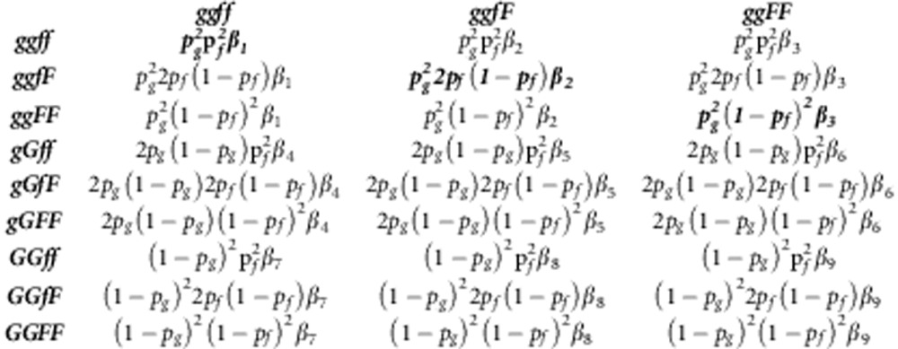
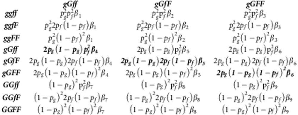
This appendix shows the construction of the NGM (Diekmann et al., 2010) and R₀ for a diploid population where there is no LD between the locus affecting susceptibility and the locus affecting infectivity. In such population, we have nine types of individuals for the combination of their genotype for susceptibility (gg, gG, GG) and infectivity (ff, fF, FF). Thus, the NGM has nine rows and nine columns. The column of the matrix represents the contributions to the next generation by infectious individuals of the genotype written above the column (‘cause'). The rows indicate the genotypes of the susceptible individuals that become infected (‘consequence'). In the following, we present the NGM on three rows: the first row gives columns 1–3, the second columns 4 –6 and the final row columns 7–9. The NGM uses the transmission rate parameters between genotypes, which are given by

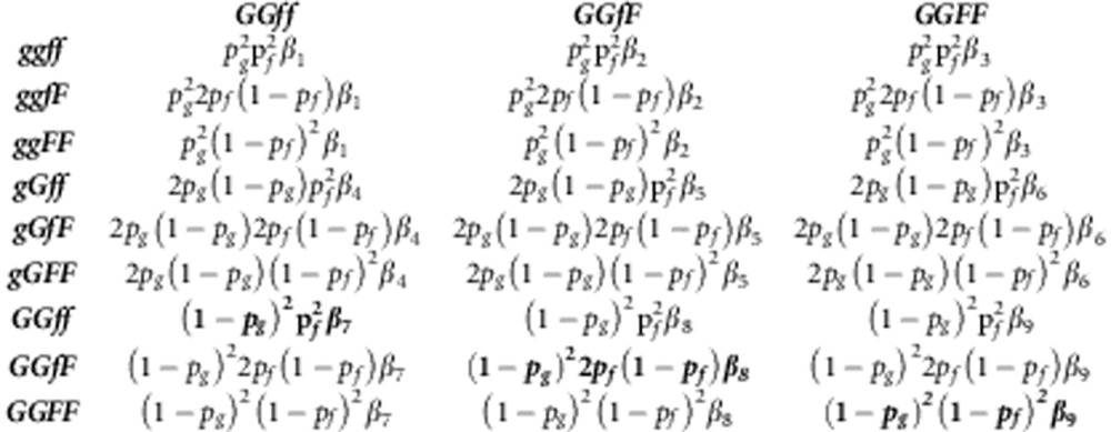R₀ is the dominant eigenvalue of the NGM. As we have the so-called separable mixing, where elements of the NGM are products of the rows and columns, the NGM has a single eigenvalue only, which therefore equals the trace of the NGM. Thus, R₀ is the sum of the diagonal elements of the NGM (given in bold above),

in which and .

Appendix 2

The NGM was also constructed for a population that deviates from LD and HWE. Because of LD, the genotype gGfF has to be partitioned into the two possible haplotypes for this genotype, gfGF and gFGf. Hence, when accounting for LD, the NGM includes 10 distinct genotypes, rather than the 9 considered in Appendix 1 (Table A2-1).

To avoid over presentation of results, we only give the trace of the NGM, which equals R₀ because of the separable mixing assumption,

Here β_vwxy represents the transmission rate parameter within a genotype, that is, from genotype vwxy to genotype vwxy,

For example, β_gFGF=γ_gGϕ_FFc.

The haplotype frequencies are

where D is the usual measure of LD (see main text).

The genotype frequencies are

After few steps of algebraic manipulation, Equation (A2-1) will reduce to

Individual breeding values for R₀ were obtained by linearizing R₀ in the allele frequencies, using partial first derivatives, and subsequently substituting individual allele frequencies (i.e. 0, 1/2 or 1)

Appendix 3

As mentioned in the main text, relatedness at the susceptibility locus, r_γ, and at the infectivity locus, r_ϕ, were allowed to be different. With a single biallelic locus, pairwise relatedness between individuals takes only three discrete values. However, our interest is in a continuum of the average relatedness among the individuals that together make up a group. To achieve a certain average relatedness among group mates, a fraction f of fully related individuals was added to each group, supplemented by a fraction 1−f of randomly selected individuals. In this appendix, we show that the required fraction equals the square root of relatedness at each locus, that is a fraction of random individuals will be replaced by individuals that were fully related to each other at the susceptibility locus, and for the infectivity locus this is a fraction . We defined relatedness as the correlation between the genotypes of two group mates, say x and y,

As the same theory applies to both loci, we will show the derivation for the susceptibility locus only.

Because the addition strategy should not change allele frequency in the population nor affect the HWE, the population needs to have three types of groups. The first type has gg individuals added to the group. The second type has gG individuals added and the third type has GG individuals added. The number of groups of the first type equals no. groups × p², the number of groups of the second type equals no. groups × 2p(1−p), and the number of groups of the third type equals no. groups × (1−p)², where p is the frequency of the g allele. The frequency of g in the three types of groups is then

To derive the correlation, we first derive the covariance between genotypic values of group members,

where, for example, E(xy|1) denotes the expectation of the product of the genotypic values of two group members in a group of type 1. To simplify the derivation, without loss of generality, g was given an effect of 1 and G an effect of 0. As we are interested in additive genetic relationship, resulting genotypic values are 2 for gg, 1 for gG and 0 for GG. Thus, x and y denote genotypic values, taking values of either 0, 1 or 2. The possible genotypes of two individuals and the corresponding values for E(xy|group type) are presented in the table below. Since the genotypic value for GG equals zero, any pair of individuals involving at least one GG individual has E(xy)=0, and is therefore left out of the table.

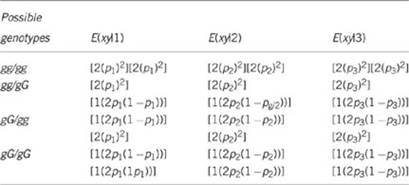
If we insert Equations (A4-2) for p₁ and Equation (A4-3) and (A4-4) for p₂ and p₃, respectively, and sum up all the elements in each of the three column for E(xy), we find

And as

Then,

Next, we need to calculate E(x) and E(y):

Then,

Then, covariance will be

Next, the variances are given by

Then, Equations (A3-1) becomes

Simplifying this expression yields

Thus, to achieve a certain relatedness, a fraction of fully related individuals should be added to each group.

Appendix 4

This appendix contains an example demonstrating the strategy to make additions in each group, so as to achieve a certain relatedness for susceptibility and infectivity among group mates. We considered 100 groups, each with 100 individuals. Let us assume that LD (D)=0.15, and that the allele frequency at susceptibility locus is 0.5 and allele frequency at infectivity locus equals 0.6. Thus, P_g=0.5 and P_f=0.6. The r_γ=0.75 and r_ϕ=0.6. It is assumed that the population is in Hardy–Weinberg equilibrium. The haplotype frequencies will be

As r=f², then the fraction f_γ of individuals that are fully related at their susceptibility locus will be . And the fraction f_ϕ of individuals that are fully related at their infectivity locus will be .

Because the required fraction is lowest for the infectivity locus, we start with the infectivity locus. Thus, in each of the 100 groups we added individuals that are fully related at their susceptibility and infectivity locus. The first 100 × f_gf² groups will contain 77 individuals with gfgf genotype, 100 × 2f_gf f_gF groups will contain 77 individuals with gfgF genotype, 100 × 2f_gf f_Gf groups will contain 77 individuals with gfGf genotype, 100 × 2f_gf f_GF groups will contain 77 individuals with gfGF genotype, groups contain 77 individuals with gFgF genotype, 100 × 2f_gF f_Gf groups will contain 77 individuals with gFGf genotype, 100 × 2f_gF f_GF groups contain 77 individuals gFGF genotype, groups will contain 77 individuals with GfGf genotype, 100 × 2f_Gf f_GF groups will contain 77 individuals with GfGF genotype and finally, groups will contain 77 individuals with GFGF.

With respect to the infectivity locus, there are p_f² × 100=36 groups that contain a fraction of individuals that are of ff, 2p_f(1−p_f) × 100=48 groups that contain a fraction of individuals that are of fF genotype and (1−p_f)² × 100=16 groups that contain a fraction of individuals that are of FF genotype at their infectivity locus. Thus, the desired additions for the infectivity locus are achieved.

With respect to the susceptibility locus, we have p_g² × 100=25 groups that contain 77 individuals that are of gg, 2p_g(1−p_g) × 100=50 groups that contain 77 individuals that are of gG genotype and (1−p_g)² × 100=25 groups that contain 77 individuals that are of FF genotype at their infectivity locus. For the susceptibility locus, however, the required number of individuals to be added equals . As we have already added 77 individuals that are fully related at their susceptibility locus, what is left to add to the group is 87−77=10 individuals Thus, the next addition will be 10 individuals that are fully related at their susceptibility locus, but taken at random with respect to their infectivity locus (so that relatedness as the infectivity locus is not affected). Therefore, for those groups that already have a fraction of individuals with gg genotype, we will add 10 more individuals that are off gg genotype. Analogously, to groups that already have a fraction of individuals with a certain genotype, 10 more individuals with that genotype are added. As the groups size is assumed to be 100, the rest of the group, which are 100−87=13 individuals, will be assigned randomly.

Appendix 5

In this appendix we presented the lower (min) and upper (max) bound for r_γ given r_ϕ and vice versa for a given LD, D. These bounds follow from the fraction of available individuals for the second addition step (see Appendix 4), which depends on the allele frequencies, D, and relatedness at the locus in the first addition step.

When D>0,

When D<0,

When D=Max (D)=±0.25,

The authors declare no conflict of interest.

References

- Anderson RM, May RM, Anderson B. Infectious Diseases of Humans: Dynamics and Control. Vol 28. Wiley Online Library; 1992. [Google Scholar]
- Bijma P. A general definition of the heritable variation that determines the potential of a population to respond to selection. Genetics. 2011;189:1347–1359. doi: 10.1534/genetics.111.130617. [DOI] [PMC free article] [PubMed] [Google Scholar]
- Bijma P, Muir WA, Van Arendonk JAM. Multilevel selection 1: quantitative genetics of inheritance and response to selection. Genetics. 2007;175:277–288. doi: 10.1534/genetics.106.062711. [DOI] [PMC free article] [PubMed] [Google Scholar]
- Bijma P, Wade M. The joint effects of kin, multilevel selection and indirect genetic effects on response to genetic selection. J Evol Biol. 2008;21:1175–1188. doi: 10.1111/j.1420-9101.2008.01550.x. [DOI] [PubMed] [Google Scholar]
- Dawkins R. The Selfish Gene. Oxford University Press: Oxford, UK; 2006. [Google Scholar]
- Diekmann O, Heesterbeek J, Roberts M. The construction of next-generation matrices for compartmental epidemic models. J R Soc Interface. 2010;7:873–885. doi: 10.1098/rsif.2009.0386. [DOI] [PMC free article] [PubMed] [Google Scholar]
- Diekmann O, Heesterbeek JAP, Metz JAJ. On the definition and the computation of the basic reproduction ratio R0 in models for infectious-diseases in heterogeneous populations. J Math Biol. 1990;28:365–382. doi: 10.1007/BF00178324. [DOI] [PubMed] [Google Scholar]
- Doeschl-Wilson AB, Davidson R, Conington J, Roughsedge T, Hutchings MR, Villanueva B. Implications of host genetic variation on the risk and prevalence of infectious diseases transmitted through the environment. Genetics. 2011;188:683–693. doi: 10.1534/genetics.110.125625. [DOI] [PMC free article] [PubMed] [Google Scholar]
- Falconer D, Mackay T.1996. C. 1996. Introduction to Quantitative Genetics, 4th edn. Longman: London.
- Fisher RA. The correlation between relatives on the supposition of Mendelian inheritance. Trans R Soc Edinburgh. 1919;52:399–433. [Google Scholar]
- Fix AG. Kin groups and trait groups: population structure and epidemic disease selection. Am J Phys Anthropol. 1984;65:201–212. doi: 10.1002/ajpa.1330650213. [DOI] [PubMed] [Google Scholar]
- Frank SA. Models of parasite virulence. Q Rev Biol. 1996;71:37–78. doi: 10.1086/419267. [DOI] [PubMed] [Google Scholar]
- Frank SA. Foundations of Social Evolution. Princeton University Press: Princeton, NJ, USA; 1998. [Google Scholar]
- Galvani AP. Epidemiology meets evolutionary ecology. Trends Ecol Evol (Personal edition) 2003;18:132–139. [Google Scholar]
- Gibson JR, Bishop SC. Use of molecular markers to enhance resistance of livestock to disease: a global approach. Rev Sci Tech Off Int Epiz. 2005;24:343–353. [PubMed] [Google Scholar]
- Griffing B. Selection in reference to biological groups.I. Individual and group selection applied to populations of unordered groups. Aust J Biol Sci. 1967;20:127–139. [PubMed] [Google Scholar]
- Griffing B. Selection in reference to biological groups. V. Analysis of full-sib groups. Genetics. 1976;82:703–722. doi: 10.1093/genetics/82.4.703. [DOI] [PMC free article] [PubMed] [Google Scholar]
- Griffing B. A theory of natural selection incorporating interaction among individuals. II. Use of related groups. J Theor Biol. 1981;89:659–677. doi: 10.1016/0022-5193(81)90034-5. [DOI] [PubMed] [Google Scholar]
- Haldane JB. Disease and evolution. La Ricerca Scientifica. 1949;19:8. [Google Scholar]
- Hamilton WD. Selfish and spiteful behaviour in an evolutionary model. Nature. 1970;228:1218–1220. doi: 10.1038/2281218a0. [DOI] [PubMed] [Google Scholar]
- Heringstad B, Chang YM, Gianola D, Klemetsdal G. Genetic association between susceptibility to clinical mastitis and protein yield in Norwegian dairy cattle. J Dairy Sci. 2005;88:1509–1514. doi: 10.3168/jds.S0022-0302(05)72819-8. [DOI] [PubMed] [Google Scholar]
- Kermack W, McKendrick A. Contributions to the mathematical theory of epidemics—I. Bull Math Biol. 1991;53:33–55. doi: 10.1007/BF02464423. [DOI] [PubMed] [Google Scholar]
- Levin S, Pimentel D. Selection of intermediate rates of increase in parasite–host systems. Am Nat. 1981. pp. 308–315.
- Lipschutz-Powell D, Woolliams JA, Bijma P, Doeschl-Wilson AB. Indirect genetic effects and the spread of infectious disease: are we capturing the full heritable variation underlying disease prevalence. PLoS ONE. 2012;7:e39551. doi: 10.1371/journal.pone.0039551. [DOI] [PMC free article] [PubMed] [Google Scholar]
- Lloyd-Smith JO, Schreiber SJ, Kopp PE, Getz WM. Superspreading and the effect of individual variation on disease emergence. Nature. 2005;438:355–359. doi: 10.1038/nature04153. [DOI] [PMC free article] [PubMed] [Google Scholar]
- Lynch M, Walsh B. Genetics and Analysis Of Quantitative Traits. Sinauer: Sunderland, MA, USA; 1998. [Google Scholar]
- Moore AJ, Brodie ED, III, Wolf JB. Interacting phenotypes and the evolutionary process: I. Direct and indirect genetic effects of social interactions. Evolution. 1997;51:1352–1362. doi: 10.1111/j.1558-5646.1997.tb01458.x. [DOI] [PubMed] [Google Scholar]
- Muir WM. Incorporation of competitive effects in forest tree or animal breeding programs. Genetics. 2005;170:1247–1259. doi: 10.1534/genetics.104.035956. [DOI] [PMC free article] [PubMed] [Google Scholar]
- O'Brien SJ, Evermann JF. Interactive influence of infectious disease and genetic diversity in natural populations. Trends Ecol Evol. 1988;3:254–259. doi: 10.1016/0169-5347(88)90058-4. [DOI] [PMC free article] [PubMed] [Google Scholar]
- Powell JE, Visscher PM, Goddard ME. Reconciling the analysis of IBD and IBS in complex trait studies. Nat Rev Genet. 2010;11:800–805. doi: 10.1038/nrg2865. [DOI] [PubMed] [Google Scholar]
- Schliekelman P. Kin selection and evolution of infectious disease resistance. Evolution. 2007;61:1277–1288. doi: 10.1111/j.1558-5646.2007.00122.x. [DOI] [PubMed] [Google Scholar]
- Wolf JB, Brodie ED, III, Cheverud JM, Moore AJ, Wade MJ. Evolutionary consequences of indirect genetic effects. Trends Ecol Evol. 1998;13:64–69. doi: 10.1016/s0169-5347(97)01233-0. [DOI] [PubMed] [Google Scholar]
- Woolhouse MEJ, Dye C, Etard J-F, Smith T, Charlwood JD, Garnett GP, et al. Heterogeneities in the transmission of infectious agents: implications for the design of control programs. Proc Natl Acad Sci USA. 1997;94:338–342. doi: 10.1073/pnas.94.1.338. [DOI] [PMC free article] [PubMed] [Google Scholar]