Comparative Identification of Differential Interactions from Trajectories of Dynamic Biological Networks

Abstract

It is often challenging to reconstruct accurately a complete dynamic biological network due to the scarcity of data collected in cost-effective experiments. This paper addresses the possibility of comparatively identifying qualitative interaction shifts between two dynamical networks from comparative time course data. An innovative approach is developed to achieve differential interaction detection by statistically comparing the trajectories, instead of numerically comparing the reconstructed interactions. The core of this approach is a statistical heterogeneity test that compares two multiple linear regression equations for the derivatives in nonlinear ordinary differential equations, statistically instead of numerically. In detecting any shift of an interaction, the uncertainty in estimated regression coefficients is taken into account by this test, while it is ignored by the reconstruction-based numerical comparison. The heterogeneity test is accomplished by assessing the gain in goodness-of-fit from using a single common interaction to using a pair of differential interactions. Compared with previous numerical comparison methods, the proposed statistical comparison always achieves higher statistical power. As sample size decreases or noise increases in a certain range, the improvement becomes substantial. The advantage is illustrated by a simulation study on the statistical power as functions of the noise level, the sample size, and the interaction complexity. This method is also capable of detecting interaction shifts in the oscillated and excitable domains of a dynamical system model describing cdc2-cyclin interactions during cell division cycle. Generally, the described approach is applicable to comparing dynamical systems of additive nonlinear ordinary differential equations.

1 Introduction

Reconstruction of gene regulatory networks or metabolic pathways from time course observations has been a sustaining focus of efforts [BBAIdB07]. Data-driven deterministic and non-deterministic mathematical modeling methods [KWKK08] have been developed to reconstruct biological networks. Examples include Bayesian networks, Boolean networks, and ordinary/partial differential equations (ODEs/PDEs). However, accurate and complete biological network reconstruction is considered beyond our current reach. This is due to several reasons, among which are the combinatory nature of the problems, limited system perturbation and un-captured dynamical measurements [Bon08]. To remediate these limitations, we take advantage of the comparative nature of many biology experimental designs, to pursue comparative identification of differential interactions.

When one inspects two models, numerical comparison (NC) of their coefficients is intuitive. As model databases such as BioModels [NBB⁺06] do not provide the data from which models are built, researchers have no choice but to use numerical comparison if they want to compare their models with those in a database. This becomes a problem when coefficients in a model have great uncertainty due to the data used to derive them. As NC methods do not consider variance in the comparison, they are effective only for accurately reconstructed networks. Therefore, several biological comparative analysis approaches have been developed [TBB07]. Differential gene expression analyses [NS04] of each single gene ignore regulatory interactions which might cause differential expression. More recently, pair-wise gene expression correlations [TBB07] utilize patterns of gene co-expression to detect gene interaction shifts. To the contrary of the NC method, correlation-based comparison considers only variance but not the way two variables interact, and would not be effective in telling the shift in interactions. Co-expressing genes can be considered as a simple model involving only two genes. Consider a network shown in the left pane of Fig. 1. A node X and a constant node C control the change of a node Y by a coefficient vector, (a, b), which are related to the correlation coefficient vector between X, C and Y. Two sets of observations {X⁽¹⁾, Y⁽¹⁾ and {X⁽²⁾, Y⁽²⁾} are obtained under different conditions which could cause changes in (a, b). In order to detect any change in (a, b), the NC method will first estimate two coefficient vectors from two data sets respectively, then compare the distance between the two estimated coefficient vectors with an experienced threshold. However, this numerical comparison may be unreliable, as illustrated by an example in the center and right panes of Fig. 1. Although the distance between the two estimated coefficient vectors is greater in the center pane than in the right pane, the data sets do not support such an interaction difference in the center pane as strong as in the right pane considering the uncertainty in the estimated coefficients. A threshold in between the two distances will lead to false negative differential interaction detection on the case in the right pane.

Figure 1.

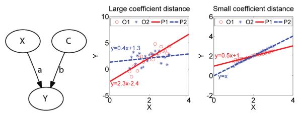
Unreliable NC estimation of the heterogeneity of an interaction from observations under two conditions. Left: An interaction with a coefficient vector, (a, b), which might shift under two conditions; Center: The observations, (O1, O2), led to estimation of a large, but insignificant, difference between the coefficient vectors. (P1, P2) are model predictions; Right: The observations, (O1, O2), let to estimation of a small, but significant, difference between the coefficient vectors.(P1, P2) are model predictions.

We establish a new paradigm of statistical comparison (SC) to detect interaction shifts in a biological network. An SC method can be considered a generalization of NC by extending the zero-variance assumption to non-zero. The significance takes the uncertainty into account that will be reported by a statistical heterogeneity test. The null hypothesis is that the interactions keep the same. A differential interaction in a network will be detected by rejecting the null hypothesis through analyzing the goodness-of-fit between a common interaction and several differential interactions. The proposed method will take uncertainty into account while focusing on the identification of interaction changes. In this paper, considering two comparable biological networks, we assume the true topology of the network is given but coefficients. We define an interaction by an ODE. A method is also given based on statistical comparison of multiple linear regression equations. Then, the performance of the proposed method will be illustrated by simulation studies under various noise levels, data sizes and interaction complexities. We also demonstrate our SC approach on a real biological network delineating cdc2-cyclin interactions in the cell division cycle.

2 Interactions in dynamical systems

We focus on detecting the interaction shifts in biological networks represented by dynamical system models (DSMs) composed of ODEs. We choose DSMs for two reasons: first, ODEs are widely used in kinetic models; second, biological model databases including a large number of DSMs, such as BioModels [NBB⁺06], have been created, which can be used to test our methods. In gene regulatory network modeling, ODEs has been used to describe transcriptional kinetics [dLD09], where gene regulation is modeled by reaction-rate equations expressing the rate of a gene product as a function of concentrations of other gene products or metabolites in the system. The general mathematical form is

$$\frac{d{x}_i\left(t\right)}{dt}{f}_i\left(\mathbf{x}\right(t),\beta )$$ (1)

where X(t) = (x₀(t), …, x_N–1(t))^⊺ is a vector of the concentrations of N variables at time t, x_i(t) is a target variable which can represent the concentration of a gene product or a metabolite, β is a coefficient constant vector, and f_i is a linear combination of either linear (e.g. x_j) or nonlinear (e.g. quadratic $x_j^2$ or x_jx_k, or sigmoidal $\frac{x_j^2}{1+x_j^2}$) terms, with coefficients β. The pair-wise linear correlation model is a special case of the above model as 0 = β₀ + x_i(t) + β₁x_j(t). Coefficient vector β in model f_i can be estimated using multiple linear regression. We also refer to this estimation process as reconstruction and estimated coefficient vector as $\widehat{\beta }$.

In a pair of differential interactions for a variable, the two coefficient vectors, β⁽¹⁾ and β⁽²⁾, differ from each other under two experimental conditions. Take Fig. 1 as an example. The values of node X, Y, and C can be considered gene concentrations. The rate of change in gene Y is regulated by X and C through a coefficient vector β = (a, b). Thus, any change in the values of (a, b) implies an interaction shift.

3 Detecting differential interactions via heterogeneity tests

We introduce the SC method and compare it with the more intuitive NC method. The NC method identifies interaction shifts in biological networks by numerically comparing with a threshold the distance between estimated coefficient vectors of individually reconstructed models based on several comparative data sets. On the other hand, the SC approach tests the interaction shifts by analyzing the goodness-of-fit of individual models (together called a heterogenous model) and a pooled model (a homogenous model) which is assumed to produce all data sets. A p-value as the significance will be reported by SC method finally.

How two methods work will be introduced by using the ODEs described in Eq. (1). Let matrix X = (x[0]^⊺, x[1]^⊺, … , x[T – 1]^⊺) be one observation set from T discrete time points. The concentration change rate, y[t], of an interested variable i at discrete time t,

$$y\left[t\right]=\frac{d{x}_i\left[t\right]}{dt}$$ (2)

will be obtained from observations by using a smoothing spline technique in this paper. Let a vector Y = (y[0], y[1], … , y[T – 1])^⊺ represent one derivative set of the interested element at T time points. Assume two sets of the concentration observations in a network under different conditions are obtained, {X⁽¹⁾, Y⁽¹⁾} and {X⁽²⁾, Y⁽²⁾}, respectively. The comparative methods can be utilized to check if these two sets come from two differential interactions while all observations contain the noise.

3.1 The numerical comparison approach

The NC method will produce a score based on the distance between individual models. After using the model reconstruction method to obtain ${\widehat{\beta }}^{\left(1\right)}$ and ${\widehat{\beta }}^{\left(2\right)}$ from two observation sets, respectively, the score will be calculated by

$${\text{Score}}_R=\sqrt{{({\widehat{\beta }}^{\left(1\right)}-{\widehat{\beta }}^{\left(2\right)})}^{⊺}({\widehat{\beta }}^{\left(1\right)}-{\widehat{\beta }}^{\left(2\right)})}$$ (3)

Based on the result of comparing this score with an experienced threshold, a differential interaction will be identified while the calculated score is larger.

There are several drawbacks of this method. Take Fig. 1 as an example, a large distance between estimated coefficients is not always associated with a difference between the true coefficients, as noise can distort the estimated difference. Furthermore, if the scales within a coefficient vector are not the same, normalization has to be applied as shown in Eq. (7).

3.2 The statistical comparison approach

We propose the SC method to identify interaction shifts in dynamic biological networks, based on a statistical heterogeneity test to compare model coefficients in two multiple linear regression models. The method detects the interaction shifts by analyzing the goodness-of-fit of a heterogenous interaction model versus a homogenous interaction model.

We formulate differential interaction detection as a statistical inference problem and obtain the best estimators first. Considering two sets of observations, {X⁽¹⁾,Y⁽¹⁾} and {X⁽²⁾,Y⁽²⁾}, we assume the best model estimators for them are ${\widehat{\beta }}^{\left(1\right)}$ and ${\widehat{\beta }}^{\left(2\right)}$ respectively, which together form a heterogenous model (with a complexity of $P_{he}={\sum }_{j=1}^2\mathit{dim}\left({\widehat{\beta }}^{\left(j\right)}\right))$). Under the null hypothesis that two data sets are from a single homogenous interaction model (with a complexity of P_ho), its best estimator is ${\widehat{\beta }}_{ho}(P_{ho}=\mathit{dim}({\widehat{\beta }}_{ho}\left)\right)$ which is calculated based on the pooled data set.

A test is now presented to test the null hypothesis of non-interaction-shift by comparing the performance of two models, though their modeling residuals respectively

$$R_{he}=\sum _{j=1}^2{({\widehat{\mathbf{Y}}}^{\left(j\right)}-{\mathbf{Y}}^{\left(j\right)})}^{⊺}({\widehat{\mathbf{Y}}}^{\left(j\right)}-{\mathbf{Y}}^{\left(j\right)}),R_{ho}=\sum _{j=1}^2{({\widehat{\mathbf{Y}}}_{ho}^{\left(j\right)}-{\mathbf{Y}}^{\left(j\right)})}^{⊺}({\widehat{\mathbf{Y}}}_{ho}^{\left(j\right)}-{\mathbf{Y}}^{\left(j\right)})$$ (4)

where first derivatives ${\widehat{\mathbf{Y}}}^{\left(j\right)}=f_i({\mathbf{X}}^{\left(j\right)},{\widehat{\beta }}^{\left(j\right)})$ is estimated by the heterogenous model with the jth data set and model coefficients; one element in Y^(j) which is obtained from observation directly is defined in Eq. (2); ${\widehat{\mathbf{Y}}}_{ho}^{\left(j\right)}=f_i({\mathbf{X}}^{\left(j\right)},{\widehat{\beta }}_{ho})$ is obtained by the homogenous model. We notice that heterogenous models become a homogenous one when ${\widehat{\beta }}^{\left(1\right)}={\widehat{\beta }}^{\left(2\right)}$ implying that the homogenous model is nested within the heterogenous one (P_ho ≤ P_he). While the model complexities are taken into account, the proportion of the performance improvement achieved by heterogenous model versus its own performance can be inspected by using the ratio

$$F=\frac{(R_{ho}-R_{he})∕d{f}_1}{R_{he}∕d{f}_2}$$ (5)

where df₁ = P_he – P_ho and df₂ = T – P_he. Under the null hypothesis, which is that both data sets are from a homogenous interaction model, the test statistic F follows an F-distribution with df₁ and df₂ degrees of freedom while the data size is asymptotic [Zar98]. If the test size α is given, using the above F-test, we can determine if two data sets arise from differential interactions. The F value is considered as the score of SC method. The significance level (p-value) in the application could be reported after obtaining the distribution of the test statistic by permutation when the sample size is small. We also point out that this method already works for comparing two additive nonlinear ODE models and can be extended to identify interaction shifts under more than two conditions.

4 Performance evaluation on simulated and real biological networks

To compare the performance of the NC and SC methods, we use the receiver operating characteristic (ROC) curve. The ROC curve is a graphical plot of the true positive rate (T P R) vs. the false positive rate (F P R) for a binary classifier as its discrimination threshold is varied. T P R is the detected fraction of all true differential interactions; while F P R is the fraction of all true non-differential interactions, that are incorrectly announced, also known as Type I error. The statistical power which is T P R at F P R = 0.05, is a function of population parameters, including but not limited to noise level, sample size, and the complexity of the classifier. A classifier whose ROC curve is closer to the top left corner has better performance, while the one that has an ROC of a diagonal line from (0,0) to (1,1) is equivalent to random guessing. One can also quantify the area under an ROC curve - a larger area indicates a better performance.

4.1 Simulation studies on the statistical power

We generated ROC curves for the SC and NC methods via a simulation study. Two types of ODE pairs were created randomly: the first type contains two identical ODEs representing conserved interactions; the second type contains two different ODEs representing differential interactions. Three coefficient vectors of dimension N+1 or complexity N (number of independent variables) were randomly sampled from uniform distribution from −5 to 5. The 1^st coefficient vector is shared by the pair of identical ODEs; the 2^nd and 3^rd are used for the pair of different ODEs. We randomly generated 300 ODE pairs for each type. For each ODE, T observations for each independent variable on the right hand side of Eq. (1) were sampled from the uniform distribution from −10 to 10; the left handside’s first derivative was calculated directly from the ODE. Trajectories were simulated from the ODEs using T observations and first derivatives. Additive noise of zero-mean normal distributions is applied repeatedly to obtain noisy replicates of the trajectories. The SC and NC methods were applied to each pair of data sets to detect differential interactions. Detection results on those pairs of data sets from the identical/different ODE pair were used to compute the FPR/TPR for plotting the ROC curve.

The performance of NC and SC methods under different noise levels are given in Fig. 2 by setting N = 1, T = 3 and σ = (0.05, 0.4, 1.5, 4). The ROC curves are displayed in the left pane of Fig. 2. Both methods had good performance when the noise was low, while when the noise was high neither had any useful result. It is evident that the SC had consistently better performance under the intermediate noise levels. The statistical power as a function of noise level, shown in the right pane of Fig. 2, is another way to visualize the SC advantage of the T P R at F P R = 0.05.

Figure 2.

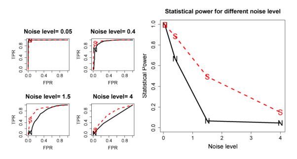
ROC and power advantage of the SC over the NC method under various noise levels. Left: ROC curves under four noise levels; Right: Power as a function of noise level. Solid curves marked by “N” represent NC, while the dashed ones marked by “S” represent SC. The noise level shown is the standard deviation of the noise.

The SC method also achieved a better performance on sample sizes and variable dimensions than the NC method, as illustrated in Fig. 3. We obtained the statistical power curves of the sample size, shown in the left pane of Fig. 3, by setting σ = 1.5 and N = 1. The statistical power curves of the independent variable dimension, shown in right pane of Fig. 3, were obtained by setting σ = 1.5 and T = 7. The statistical power gain of SC over NC in the two situations is up to 50% and 70%, respectively - an extraordinary advantage.

Figure 3.

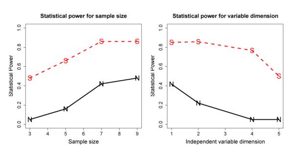
Power advantage of the SC over the NC method under various sample size and interaction complexity. Left: Statistical Power as a function of the sample size; Right: Statistical Power as a function of independent variable dimension. The solid curves marked by “N” represent NC, while the dashed ones marked by “S” represent SC.

4.2 Differential interactions between cdc2 and cyclin in a cell division cycle model

As difference in trajectories under comparative conditions is insufficient to imply mechanism shifts in a dynamic biological network, one must examine the interactions at each node and check if any of them have changed in their coefficients. Thus we examine the heterogeneity of interactions at each node one by one in the network. We use a dynamical system model (Fig. 4) of cdc2-cyclin interaction in the cell division cycle [Tys91] to illustrate the performance of the two comparison methods on detecting mechanism shifts in the network. The cdc2-cyclin dynamical system model consists of six kinetic equations, shown in Table 1. Following recommendations for coefficient values in [Tys91], we set k₁[aa]/[CT] = 0.015min⁻¹, k₂ = 0, k₃[CT] = 200min⁻¹, $k_4^{\prime }=0.018{\mathit{min}}^{-1}$, k₅[~ P] = 0, k₆ = 1min⁻¹, k₇ = 0.6min⁻¹, k₈[~ P] = 1000000min⁻¹ and k₉ = 1000min⁻¹, where [CT] was assumed to be a constant of 1. In this study, we perturb the coefficient k₄, a rate constant associated with the autocatalytic activation of MPF by dephosphorylation of the cdc2 subunit [Tys91], marked as reaction 4 in Fig. 4. After cell division becomes growth controlled, k₄ > 150min⁻¹, MPF enters the oscillation domain in which it alternates between active and inactive forms with a period of 35 min, roughly the cell cycle length in early frog embryos [Tys91]. While k₄ < 100min⁻¹, MPF, being maintained in inactive forms, goes into the excitable domain (as in the resting phase of non-proliferating somatic cells). As cells grow, k₄ increases (activator accumulates) and drives the regulatory system into the oscillation domain. The subsequent burst of MPF activity triggers mitosis, causes k₄ to decrease (activator degrades), and brings the regulatory system back into the excitable domain (steady-state behavior). We use the comparison methods to detect changed interactions due to k₄, which implicates two differential interactions for preMPF and active MPF. The remaining interactions for other four proteins are conserved.

Figure 4.

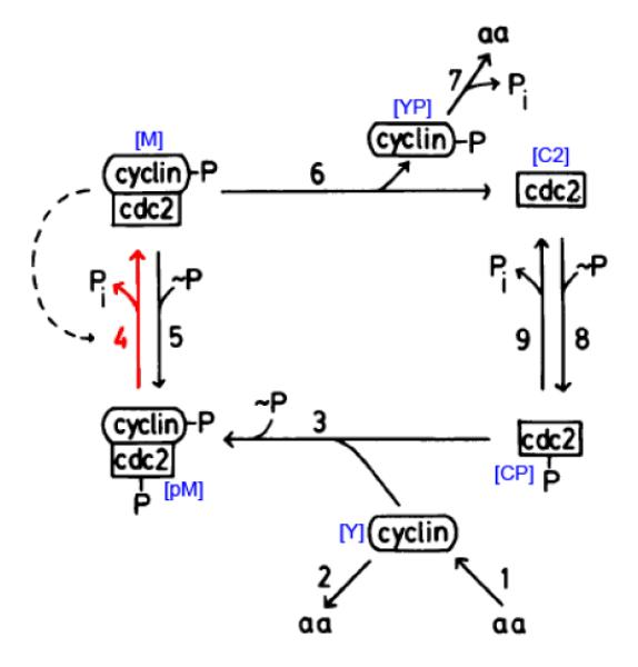
The cdc2-cyclin interaction dynamic network involved in the cell division cycle [Tys91]. The variable names used in the dynamical system model (Table 1) are marked next to the proteins or protein complexes they represent. The network shifts in the interaction change marked by #4.

Table 1.

ODEs governing the cdc2-cyclin interaction in the cell division cycle [Tys91]: t, time; k_i, rate constant; aa, amino acids. The concentrations [aa] and [~ P] are assumed to be constant. Variable [C2] is for cdc2, [CP] for cdc2-P, [pM] for preMPF=P-cyclin-cdc2-P, [M] for active MPF (P-cyclin-cdc2), [Y] for cyclin and [YP] for cyclin-P, and [CT] for total cdc2.

d[C2]/dt = k6[M] – k8[~ P][C2] + k9[CP]

d[CP]/dt = −k3[CP][Y] + k8[~ P][C2] – k9[CP]

d[pM]/dt = k3[CP][Y] $k_4^{\prime }\left[pM\right]$ – k4[pM]([M/[CT])2

d[M]/dt = $k_4^{\prime }\left[pM\right]$ + k4[pM]([M]/[CT])2 – k5[~ P][M]–k6[M]

d[Y]/dt = k1[aa] – k2[Y] – k3[CP][Y]

d[YP]/dt = k6[M] – k7[YP]

As the observed trajectories for the 6 involved proteins are distinctive in the two domains of the cell division cycle, differential gene expression analysis would report statistically significant changes in all proteins. We applied the NC and SC methods to detect differential interactions for [pM] and [M] as well as conserved interactions of other proteins. k₄ was set to be 180 min⁻¹ in the oscillation domain, while in the excitable domain, k₄ was randomly chosen from a uniform distribution from 70 to 80. After 20 observations of 40-min long trajectories were obtained for each domain, noises were added three times to generate replicates. A smoothing spline technique was utilized to obtain the first derivatives for each variable from the noisy observations. Assuming that the forms of kinetic equations were known but not the coefficients, both methods were applied to detect differential interactions of each protein in the network with varying thresholds under four noise levels. Then we compared the detection results with the two true differential interactions at [pM] and [M] (true positives) and four true conserved interactions at [C2], [CP], [Y] and [Y P] (true negatives) to compute the overall T P R and F P R at each noise level.

The noise level in this study is represented by signal-to-noise ratio (SNR), defined as ten times log₁₀ of the sum of squares of the signal divided by the sum of squares of the noise. When the data sets contain replicates, the SNR can be estimated by

$$\mathit{SNR}=10{\log }_{10}{\left(\frac{\sum _{i=1}^K{\stackrel{‒}{O}}_{i\cdot }}{\sum _{i=1}^K\left(\sum _{j=1}^{M_i}\right(O_{ij}-{\stackrel{‒}{O}}_{i\cdot })∕M_i)}\right)}^2$$ (6)

where O_ij means the j-th replicate of i-th observation, among a total of K observations, the i-th observation contains M_i replicates, and ${\stackrel{‒}{O}}_{i\cdot }=\frac{1}{M_i}{\sum }_{j=1}^{M_i}{O}_{ij\cdot }$.

As the scales of coefficients were different, we modified the NC score from Eq. (3) to

$${\text{Score}}_R=\underset{i=1,\dots ,N}{\max }(\mid {\widehat{\beta }}_i^{\left(1\right)}-{\widehat{\beta }}_i^{\left(2\right)}\mid ∕(2\max ({\widehat{\beta }}_i^{\left(1\right)},{\widehat{\beta }}_i^{\left(2\right)})\left)\right)$$ (7)

where N is the dimension of $\widehat{\beta }$.

The SC method achieved consistently and significantly better performance than the NC method on differential interaction detection in networks. From Fig. 5, we can see when the noise was low (SNR = 45dB), both methods achieved good performance. However, when the noise strength increased (SNR = 35, 25, 20dB), the performance of NC method dropped very quickly, while the SC maintained above 80% power at a type I error of 0.05.

Figure 5.

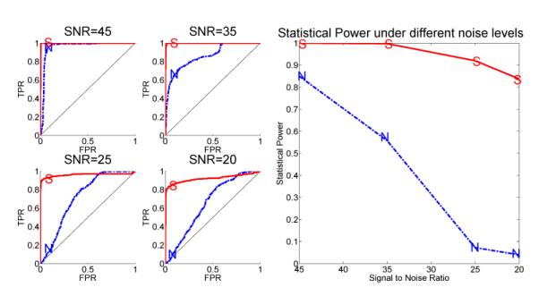
The advantage in ROC curves and statistical power of the SC (marked by “S”) versus the NC methods (marked by “N”) to detect differential interactions in the cdc2-cyclin cell division cycle model. Left: The ROC curves under different noise levels. Right: The statistical power of both methods as a function of the noise level.

5 Discussion

We have proposed an SC method to identify differential interactions in nonlinear dynamic biological networks, based on a statistical test to compare multiple linear regression equations. In addition to be able to announce two networks are different, the method can also detect which node in the network has experienced an interaction shift. Our simulation studies demonstrated that the performance of SC approach is substantially superior to the NC method under various noise levels, sample sizes, and interaction complexities. The cdc2-cyclin interaction cell division cycle model was also used to test the proposed method on real biological networks and our method achieved much improved identification accuracy of differential interactions over the NC method. The SC method is much more sensitive to detect consistent interaction changes while keeping a low Type I error.

Our comparative modeling is capable of generating two lists: one is a list of the genes whose regulatory relationships from a common concerting theme under the comparative conditions, such as [C2], [CP], [Y] and [Y P] in the cell cycle model; the other is the list of genes whose regulatory relationships consistently demonstrated distinctive signatures under the comparative conditions, such as [pM] and [M] in the cell cycle model.

We are working on applying the proposed method on studying differential gene interactions between embryonic and postnatal stages in mouse cerebellar development. We anticipate our approach widely applicable to many comparative experimental designs in life science research.

References

- [BBAIdB07].Bansal M, Belcastro V, Ambesi-Impiombato A, di Bernardo D. How to infer gene networks from expression profiles. Mol Syst Biol. 2007;3(78) doi: 10.1038/msb4100120. [DOI] [PMC free article] [PubMed] [Google Scholar]
- [Bon08].Bonneau R. Learning biological networks: from modules to dynamics. Nature Chemical Biology. 2008 Nov;4(11):658–664. doi: 10.1038/nchembio.122. [DOI] [PubMed] [Google Scholar]
- [dLD09].Ben-Tabou de Leon S, Davidson EH. Modeling the dynamics of transcriptional gene regulatory networks for animal development. Developmental Biology. 2009 Jan;325(2):317–328. doi: 10.1016/j.ydbio.2008.10.043. [DOI] [PMC free article] [PubMed] [Google Scholar]
- [KWKK08].Kestler HA, Wawra C, Kracher B, Kühl M. Network Modeling of Signal Transduction: Establishing the Global View. Bioassays. 2008 Nov;30(11-12):1110–1125. doi: 10.1002/bies.20834. [DOI] [PubMed] [Google Scholar]
- [NBB+06].Le Novre N, Bornstein B, Broicher A, Courtot M, Donizelli M, Dharuri H, Li L, Sauro H, Schilstra M, Shapiro B, Snoep JL, Hucka M. BioModels Database: a free, centralized database of curated, published, quantitative kinetic models of biochemical and cellular systems. Nucleic Acids Res. 2006 Jan;34(Database Issue):D689–D691. doi: 10.1093/nar/gkj092. [DOI] [PMC free article] [PubMed] [Google Scholar]
- [NS04].Neuhäuser M, Senske R. The Baumgartner-Weiβ-Schindler test for the detection of differentially expressed genes in replicated microarray experiments. Bioinformatics. 2004;20(18):3553–3564. doi: 10.1093/bioinformatics/bth442. [DOI] [PubMed] [Google Scholar]
- [TBB07].Tirosh I, Bilu Y, Barkai N. Comparative biology: beyond sequence analysis. Current Opinion in Biotechnology. 2007 Aug;18(4):371–377. doi: 10.1016/j.copbio.2007.07.003. [DOI] [PubMed] [Google Scholar]
- [Tys91].Tyson JJ. Modeling the cell division cycle: cdc2 and cyclin interactions. Proceedings of the National Academy of Sciences. 1991 Aug;88(16):7328–7332. doi: 10.1073/pnas.88.16.7328. [DOI] [PMC free article] [PubMed] [Google Scholar]
- [Zar98].Zar JH. Biostatistical Analysis. 4th edition Prentice Hall; Oct, 1998. [Google Scholar]