Efficient fully 3D list-mode TOF PET image reconstruction using a factorized system matrix with an image domain resolution model

Abstract

A factorized system matrix utilizing an image domain resolution model is attractive in fully 3D TOF PET image reconstruction using list-mode data. In this paper, we study a factored model based on sparse matrix factorization that is comprised primarily of a simplified geometrical projection matrix and an image blurring matrix. Beside the commonly-used Siddon's raytracer, we propose another more simplified geometrical projector based on the Bresenham's raytracer which further reduces the computational cost. We discuss in general how to obtain an image blurring matrix associated with a geometrical projector, and provide theoretical analysis that can be used to inspect the efficiency in model factorization. In simulation studies, we investigate the performance of the proposed sparse factorization model in terms of spatial resolution, noise properties and computational cost. The quantitative results reveal that the factorization model can be as efficient as a nonfactored model such as the analytical model while its computational cost can be much lower. In addition we conduct Monte Carlo simulations to identify the conditions under which the image resolution model can become more efficient in terms of image contrast recovery. We verify our observations using the provided theoretical analysis. The result offers a general guide to achieve optimal reconstruction performance based on a sparse factorization model with an only image domain resolution model.

1. Introduction

Time-of-flight (TOF) PET has become the state of the art for clinical PET imaging. list-mode reconstruction technique is the preferred choice of image reconstruction for TOF PET due to the large number of lines of response (LOR). To avoid the storage of a huge system matrix, list-mode reconstruction often calculates lines of response (LOR) on-the-fly (Popescu et al. 2004, Hu et al. 2006, Wang et al. 2006, Pratx et al. 2011, Pratx and Levin 2011). However, the accuracy of on-the-fly calculations is limited because of the constraint on image reconstruction time. While there have been some work of using parallel computing techniques such as distributed computing (Hu et al. 2006) and the graphics processing unit (GPU) to accelerate the processing speed (Pratx et al. 2011, Pratx and Levin 2011, Cui et al. 2011), the achievable accuracy of the on-the-fly calculations is still worse than a precomputed system model.

Alternatively, we propose to use a factorized model in place of the accurate model. A typical factorized system model has three major components: a sinogram blurring matrix, a geometrical projection matrix and an image blurring matrix. The geometrical projection matrix provides the mapping from the image space to the projection space. The two blurring matrices model the blurring effects in the sinogram domain and image domain, respectively. Many existing work use only one blurring matrix in conjunction with a geometrical projection matrix. For example, only the sinogram blurring matrix was used in (Mumcuoglu et al. 1996, Qi et al. 1998, Panin et al. 2006, Alessio et al. 2006, Tohme and Qi 2009, Alessio et al. 2010), while the image blurring matrix was used in (Sureau et al. 2008, Rapisarda et al. 2010, Cloquet et al. 2010, Stute and Comtat 2013). We have shown in (Zhou and Qi 2011) that using both blurring matrices, we can use a much simpler geometrical projection matrix to accelerate the projection speed without sacrificing the image quality. However, because the sinogram blurring matrix is defined in the complete projection space, it is incompatible with list-mode data format. Hence the image blurring matrix is the only choice for list-mode image reconstruction.

Most of the existing work on factorized system model concerns non-TOF image reconstruction. Here we study the factorized system model with an image blurring kernel for TOF PET. We investigate two simple geometrical projection models. One is the popular Siddon's ray-tracer (Siddon 1985) and the other is the Bresenham's algorithm (Bresenham 1965), which is even faster than the Siddon's ray-tracer. By tailoring the image burring matrix for the particular choice of the geometrical projection matrix, the blurring matrix not only models the point spread function of the PET scanner, but also corrects the sampling artifacts of the geometrical projector. We evaluate our methods by reconstruction of Monte Carlo simulated data. The results show that with a properly constructed image blurring matrix, the two geometrical projectors achieve similar image quality. In addition to simulation studies, we also provide a theoretical analysis of the model accuracy, because an exact matrix factorization usually does not exist. We provide a method to check model accuracy and verify it for different geometric projectors and voxel sizes. The results will be useful for the optimal design of image-based system factorization model for PET reconstruction.

This paper is organized as follows. In Section 2, we discuss an accurate TOF LOR model and then propose our factorized system model. We also describe in detail the two geometrical projectors, the estimation of image blurring matrix and model normalization. In Section 3, we conduct experimental studies including spatial resolution, noise properties and computational cost. Finally, discussion and conclusions are presented in Section 4 .

2. Theory

An accurate TOF system matrix can be calculated analytically, if inter-crystal scatter effect, photon acollinearity, and position range effect are negligible. Our derivation is based on the previous work for non-TOF PET (Huesman et al. 2000), which models the solid angle effect and parallax error caused by crystal penetration and finite crystal width. It has been shown to track the resolution broadening in the radial direction fairly well when compared to experimental measurements (Tohme and Qi 2006) . We extend it to TOF PET and obtain the probability of coincidence photon emitted from voxel j and detected by crystal pair i with time difference Δτ,

$$p_{\mathit{\text{ij}}}(\Delta \tau )\approx a_o^i{\kappa }_{\sigma }(\frac{2u_j^i}{c}-\Delta \tau ){\int }_{V_0}{\int }_{V_1}\frac{a_d^i({\overrightarrow{\upsilon }}_0,{\overrightarrow{\upsilon }}_1)}{{\Vert {\overrightarrow{\upsilon }}_1-{\overrightarrow{\upsilon }}_0\Vert }^2}{\int }_{L({\overrightarrow{\upsilon }}_0,{\overrightarrow{\upsilon }}_1)}{b}_j(\ell )d\ell d{\overrightarrow{\upsilon }}_{0}d{\overrightarrow{\upsilon }}_1.$$ (1)

where $a_o^i$ accounts for the object attenuation for the ith LOR. κ_σ is the timing window function. Here we model it as a Gaussian function with a standard deviation of σ. $u_j^i$ is the distance of voxel j from the center of LOR i and c is the speed of light. V₀ and V₁ denote the volumetric regions of the two crystals forming LOR i. υ⃗₀ and υ⃗₁ are interaction points inside the two crystals respectively. $a_d^i({\overrightarrow{\upsilon }}_0,{\overrightarrow{\upsilon }}_1)$ represents the joint probability of two photons penetrating through the detector material and respectively reaching points υ⃗₀ and υ⃗₁. L(υ⃗₀, υ⃗₁) is the line defined by υ⃗₀ and υ⃗₁ and b_j(·) is the basis of function of voxel j. If there is no timing window function, Eq. (1) reduces to the probability for the non-TOF case. Therefore, a TOF LOR is roughly equal to a non-TOF LOR weighted by a timing window function. As a result, a TOF projector can be implemented using a non-TOF system matrix with the timing window function computed on-the-fly.

2.1. System matrix factorization

Accurate TOF LOR can be stored row by row to form an accurate system matrix denoted by P_{TOF − acc}. For fast reconstruction, we seek a factored system model to approximate the accurate system matrix. The factored system model has the form of

$${\mathit{P}}_{\mathit{\text{TOF}}-\mathit{\text{FA}}}=\text{diag}\left\{{\mathit{n}}_{\text{TOF}}\right\}{\mathit{G}}_{\text{TOF}}\mathit{R}$$ (2)

where diag{n_TOF} is the diagonal matrix whose diagonal contains normalization factors stored in the vector n_tof, G_tof is the TOF geometrical projection matrix, and R is the image blurring matrix. The factorization may be done in a completely blind way that assumes all factors are unknown, but for simplicity we often consider a given G_TOF and then estimate n_tof and R. Usually ntof is assigned to the element-by-element ratio of the forward projections of a uniform source by P_{TOF − acc} and G_TOF, respectively, i.e. n_tof = [P_{TOF − acc}1]/[G_TOF1], where 1 is an all one vector.

2.2. Geometrical projection matrix

To accelerate the projection speed, the LOR in G_tof may be calculated simply by a line integral rather than a volume integral:

$$g_{\mathit{\text{ij}}}(\Delta \tau )={\int }_{L_i}{b}_j(\ell ){\kappa }_{\sigma }(\Delta \tau -\ell )d\ell$$ (3)

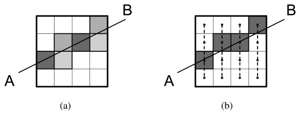
where L_i is a line connecting the centers of the crystals forming LOR i. We consider the commonly used cubic voxel and evaluate the integral using the intersection length between the line and the voxel. This is illustrated in figure 1(a). The intersection length can be calculated efficiently by using Siddon's method (Siddon 1985) or its variants.

Figure 1.

(a) A 2D illustration of the Siddon's raytracer which goes from A to B passing through an image of size 4 × 4. The gray pixels indicate nonzero voxels along the line. The gray level is proportional to the intersection length of line AB with the voxel, i.e., the darker the color is, the longer the length is. (b) An example of the Bresenham's method generating a line from A to B. All these voxels have the same value as they are in the same color.

To achieve an even faster projection speed, we investigate another line projector based on Bresenham's method (Bresenham 1965). An illustrative example is shown in figure 1(b). First the image is split according to the slope of line AB. In the 2D case, the image can be split into columns or rows depending on the slope k. If |k| < 1, the image is split into columns; otherwise it is split into rows. In this example, the image is split into 4 columns. Each column can be viewed as a line segment which passes through the voxel center (as shown by the dash line). Then the intersection points of line AB with these line segments can be computed analytically. The voxel of each column which is nearest to the intersection point is picked up and assigned a value. The value is computed as the inverse of the cosine of the angle between line AB and the horizontal axis. As we can see, the Bresenham's method requires less number of nonzeros compared to the Siddon's method. Also note that the number of nonzeros in the Bresenham's ray-tracer is equal to the minimal number of voxels for an unbroken digital line, which indicates that the Bresenham's raytracer is potentially the one that leads to the most sparse geometrical projection matrix.

2.3. Estimation of the Image blurring matrix

Let r_j be the blurring kernel at voxel j, i.e., the jth column of matrix R. We estimate r_j by solving

$${\widehat{\mathit{r}}}_j=arg\underset{{\mathit{r}}_j\ge 0}{max}\mathrm{\Phi }({\mathit{P}}_{\text{TOF}-\mathit{\text{acc}}}{\mathit{e}}_j,\text{diag}\{{\mathit{n}}_{\text{TOF}}\}{\mathit{G}}_{\text{TOF}}{\mathit{r}}_j)$$ (4)

where Φ(y, ȳ) is the negative Kullback-Leibler (KL) distance (Byrne 1993)

$$\mathrm{\Phi }(\mathit{y},\overline{\mathit{y}})=\sum _i(y_{i}log({\overline{y}}_i/y_i)-{\overline{y}}_i+y_i),$$ (5)

and e_j is the jth unit vector (or the point source at voxel j). The optimization problem can be solved by the maximum likelihood (ML) expectation-maximization (EM) algorithm for emission tomography (Shepp and Vardi 1982). Since P_{TOF − acc}e_j is deterministic, the solution is not an ML estimate.

The huge size of the TOF system matrix may results in high computation cost. Because TOF does not affect PET spatial resolution, we propose using the non-TOF system matrix to perform the estimation as follows:

$${\widehat{\mathit{r}}}_j=arg\underset{{\mathit{r}}_j\ge 0}{max}\mathrm{\Phi }({\mathit{P}}_{\text{non}-\text{TOF}-\text{acc}}{\mathit{e}}_j,\text{diag}\{{\mathit{n}}_{\text{non}-\text{TOF}}\}{\mathit{G}}_{\text{non}-\text{TOF}}{\mathit{r}}_j).$$ (6)

We see that forming a complete R requires point source scans at every voxel location, which can be impractical to obtain. Here we assume that the blurring effect is separable in the transaxial and axial directions so only two small-size matrices, a transaxial image blurring matrix and an axial image blurring matrix, are required. Because of the separability, we only need to estimate the transaxial kernels for the voxels in the center transaxial plane and the axial kernels for the voxels on the scanner axis. Details can be found in (Zhou and Qi 2011).

2.4. Model accuracy

The most important factor that affects the accuracy of the factorization is G_TOF. We rewrite the factored model in (2) as P_{TOF − FA} = G̃_TOF R, where G̃_TOF = diag {n_TOF} G_TOF. It follows that if the range of P_{TOF − acc} is inside the range of G̃_TOF, then there exists a unique R such that P_{TOF − acc} = P_{TOF − FA}. This range condition was previously discussed in (Cloquet et al. 2010). To check the range condition for a particular choice of G̃_TOF, one can verify if each column of P_{TOF − acc} belongs to the range space of G̃_TOF . This can be done by computing the linear correlation coefficient (CC) between the jth column, P_{TOF − acc} e_j, and its projection onto the range space of G̃_TOF, ${\stackrel{\sim }{\mathit{G}}}_{\text{TOF}}{({\stackrel{\sim }{\mathit{G}}}_{\text{TOF}}^T{\stackrel{\sim }{\mathit{G}}}_{\text{TOF}})}^{-1}{\stackrel{\sim }{\mathit{G}}}_{\text{TOF}}^T{\mathit{P}}_{\text{TOF}-\mathit{\text{acc}}}{\mathit{e}}_j$. A CC of one means that the jth column belongs to the range space of G̃_TOF. The greater the CC value is, the less error there is in the factorized model. We note that ${\mathit{r}}_j^{\mathit{\text{LS}}}\equiv {({\stackrel{\sim }{\mathit{G}}}_{\text{TOF}}^T{\stackrel{\sim }{\mathit{G}}}_{\text{TOF}})}^{-1}{\stackrel{\sim }{\mathit{G}}}_{\text{TOF}}^T{\mathit{P}}_{\text{TOF}-\mathit{\text{acc}}}{\mathit{e}}_j$ is the least squares (LS) estimate of the image blurring kernel, so the CC can be simply computed between the true point source projection P_TOF−acce_j and the forward projection of the image blurring kernel, ${\stackrel{\sim }{\mathit{G}}}_{\text{TOF}}{\mathit{r}}_j^{\mathit{\text{LS}}}$. We also extend the CC calculation to image blurring kernels that we obtained using other methods, such as EM algorithm. This leads to the following expression of CC

$${\text{CC}}_j=\frac{{({\mathit{P}}_{\text{TOF}-\mathit{\text{acc}}}{\mathit{e}}_j)}^T{\stackrel{\sim }{\mathit{G}}}_{\text{TOF}}{\mathit{r}}_j}{\Vert {\mathit{P}}_{\text{TOF}-\mathit{\text{acc}}}{\mathit{e}}_j\Vert \Vert {\stackrel{\sim }{\mathit{G}}}_{\text{TOF}}{\mathit{r}}_j\Vert }$$ (7)

which can be used to access the accuracy of the factored system matrix. It was shown in (Rahmim et al. 2013) that the LS image blurring kernel can result in an unbiased image (i.e., perfect resolution recovery), but with higher variance, if the range condition is not satisfied. Such variance amplification will be reflected in the CC defined above.

3. Simulation study

3.1. Scanner geometry

We simulated a Philips Gemini TF PET system whose system parameters have been reported in (Surti et al. 2007). It has 28 detector blocks mounted on a ring of diameter 90.34 cm. Each block contains a 23 × 44 LYSO crystal array with crystal size 4 mm (transaxial) × 4 mm (axial) × 22 mm (depth). The diameter of the transaxial field of view (FOV) is about 57.6 cm while the size of the axial FOV is about 18 cm. Full scanner simulations were performed in SimSET (Lewellen et al. 1998). The simulation modeled positron range of ¹⁸F, photon acollinearity, and inter-crystal scatter effects. For the TOF data, we set the timing resolution to 585 ps. The measured true time difference of each coincidence pair was first blurred using a Gaussian timing kernel with a full-width-at-half-maximum (FWHM) equal to the preset timing resolution, and then discretized into bins of 25 ps each. To model the finite timing bin size, the actual timing window function we used is the Gaussian timing kernel function convolved with the rectangle timing bin function.

3.2. System matrix calculation and blurring kernel comparison

For accurate TOF PET image reconstruction, we used the TOF projector described in Section 2 with a precomputed non-TOF system matrix by dividing each crystal into 5 × 5 × 25 sub-elements to perform the numerical volume integration. The resulting system matrix was compressed with symmetries to reduce the storage size. All sparse matrices were saved in a compressed row storage (CRS) sparse matrix format. The timing window was calculated on-the-fly with a ±3σ truncation during the TOF reconstruction. We referred to this model as ‘TOF-acc’ and use ‘non-TOF-acc’ for the non-TOF reconstruction.

To demonstrate the accuracy of the proposed system model in (1), we forward projected five point source and compared the resulting sinograms with SimSET simulation results. Because SimSET simulation and analytical calculation used the same timing window function, we compared only non-TOF sinograms. The results are shown in Figure 2. As we can see, the two sinograms are very similar. The profiles shown in Figure 2(c) also confirms a good agreement between the analytical calculation and the Monte Carlo simulation. The Monte Carlo simulation profiles have slightly longer tails than the analytical results, which is caused by the inter-crystal scatters that is not modeled in the analytic calculation.

Figure 2.

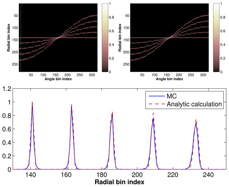
Comparison between SimSET simulation and analytical calculation. (a) SimSET simulated point source sinograms; (b) analytical calculated point source sinograms; and (c) profiles through the vertical line shown in (a).

For the factored model, we used either the Siddon's raytracer or the Bresenham's raytracer to calculate the TOF geometrical projection on-the-fly. For each raytracer, we estimated a customized image blurring matrix by running 300 ML EM iterations. The computation time to form a complete image blurring matrix was about two hours. The resulting factored system matrix are referred to as ‘TOF-Siddon/R+’ and ‘TOF-Bresenham/R+’, respectively. Also we use ‘TOF-Siddon/R-’ and ‘TOF-Bresenham/R-’ to denote the reconstructions without image resolution model. Similar notations are also used for the non-TOF case.

Figure 3(a) and (b) show the estimated kernels for the two geometrical projectors with 2 mm voxels. Only a subset of the kernels in the first quadrant is shown for better visualization. We can see that the kernels are elongated along the radial direction at radially off-center positions. Visually the two kernel images appear similar, but difference becomes evident in the subtraction image shown in Figure 3(c) as each set of kernels contain information unique to their respective geometrical projector. To show the effect of an unmatched kernel, we simulated a 2D phantom (figure 4(a)) and forward projected it using P_{TOF − acc} without adding noise. Then we reconstructed the sinogram data using the Siddon's raytracer with its own kernels as well as the kernels estimated for the Bresenham projector. We ran 300 ML-EM iterations for the image reconstruction. The results are shown in figure 4(b)-(e). Compared with the image using the matched kernels ((b) and (d)), the reconstructed image using the unmatched kernels ((c) and (e)) has more pronounced streaky artifacts.

Figure 3.

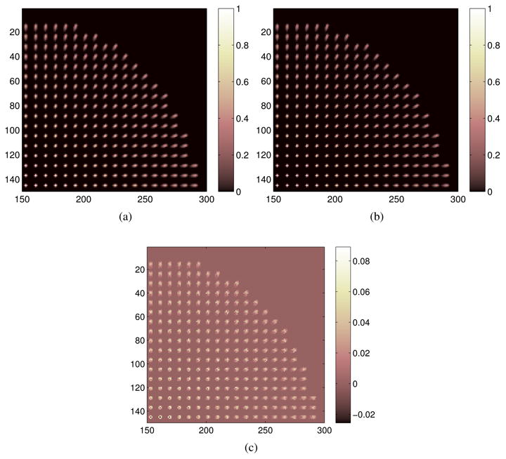
(a) The blurring kernels estimated using the Siddon's raytracer; (b) The blurring kernels estimated using the Bresenham's raytracer; (c) The kernel difference image.

Figure 4.

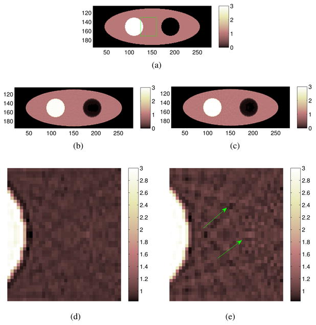
Comparison of image reconstruction using a matched and an unmatched image blurring matrix. (a) The simulated phantom image which consists of a warm background, a hot region and a cold region; (b) reconstructed image using the matched image blurring matrix; (c) reconstructed image using the unmatched image blurring matrix. (d) and (e) are zoom-in images corresponding to (b) and (c), respectively. The zoom-in area is marked by the rectangle in (a). The arrows in (e) point to the artifacts which are more pronounced than those in (d).

3.3. Spatial resolution

We evaluated the spatial resolution of different system models. Ten ¹⁸F point sources were simulated inside a warm background. We used small voxel size (∼ 0.5 mm) to simulate the point source. Five points were placed on the central transaxial plane. They were aligned horizontally starting from the center of the FOV with a uniform spacing of 6 cm. Another set of five point sources was placed in the image plane that was 6 cm off-center axially. Point source prompts and background prompts were generated separately. The total number of prompts were about 120 million and the ratio was tuned manually so that the reconstructed point source showed a reasonable contrast. For the resolution study, we only used true coincidence counts and included the attenuation effect of the warm background. No scatters and randoms were considered. For the image reconstruction, we ran 5 iterations of the ordered-subsets list-mode EM (OS-LMEM) with 20 subsets. All images were reconstructed into an array of 300 × 300 × 89 voxels with a voxel size of 2.0 × 2.0 × 2.0 mm³.

Figure 5 shows the reconstructed point sources. For better comparison, we also plotted the radial profiles across each point source. We see that the profiles are visually identical. The difference between two factored models is indistinguishable, which shows that the performance of either factored system model is quite close to that of the non-factored model.

Figure 5.

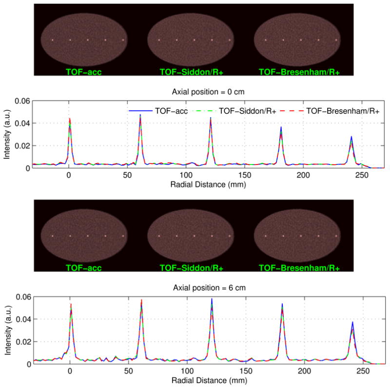
A comparison of spatial resolution of TOF-based reconstruction using different system models. Voxel size: 2 × 2 × 2 mm³.

For quantitative analysis, we measured the FWHM of each point source using Gaussian fitting. The radial, tangential and axial FWHMs were calculated and listed separately in Tab.1. In general, the factored model can well preserve the spatial resolution. The maximum difference between the factored model and the nonfactored model is only about 15%. The spatial resolution achieved by the two factored models are very similar.

Table 1.

Measured spatial resolution for each point source based on different system models.

(a) Radial FWHMs (mm)
Axial position	0 cm
Radial distance	0 cm	6 cm	12 cm	18 cm	24 cm
TOF-acc	2.53	2.53	2.59	3.00	3.58
TOF-Siddon/R+	2.57	2.70	2.71	3.27	3.68
TOF-Bresenham/R+	2.44	2.67	2.76	3.33	3.78
Axial position	6 cm
Radial distance	0 cm	6 cm	12 cm	18 cm	24 cm
TOF-acc	2.99	3.22	3.15	3.67	4.28
TOF-Siddon/R+	3.15	3.21	3.45	3.83	4.44
TOF-Bresenham/R+	2.98	3.07	3.74	3.81	4.47

(b) Tangential FWHMs (mm)
Axial position	0 cm
Radial distance	0 cm	6 cm	12 cm	18 cm	24 cm
TOF-acc	2.50	2.44	2.61	2.79	2.99
TOF-Siddon/R+	2.58	2.59	2.65	3.00	3.28
TOF-Bresenham/R+	2.48	2.66	2.69	3.01	3.30
Axial position	6 cm
Radial distance	0 cm	6 cm	12 cm	18 cm	24 cm
TOF-acc	2.59	2.70	2.51	2.61	2.80
TOF-Siddon/R+	2.70	2.75	2.69	2.72	3.16
TOF-Bresenham/R+	2.57	2.72	2.78	2.77	3.27

(c) Axial FWHMs (mm)
Axial position	0 cm
Radial distance	0 cm	6 cm	12 cm	18 cm	24 cm
TOF-acc	2.22	2.37	2.33	2.30	2.31
TOF-Siddon/R+	2.26	2.49	2.42	2.51	2.46
TOF-Bresenham/R+	2.27	2.51	2.44	2.56	2.46
Axial position	6 cm
Radial distance	0 cm	6 cm	12 cm	18 cm	24 cm
TOF-acc	3.68	3.11	3.23	3.30	3.33
TOF-Siddon/R+	3.77	3.55	3.30	3.42	3.58
TOF-Bresenham/R+	3.75	3.54	3.29	3.51	3.66

3.4. Noise properties

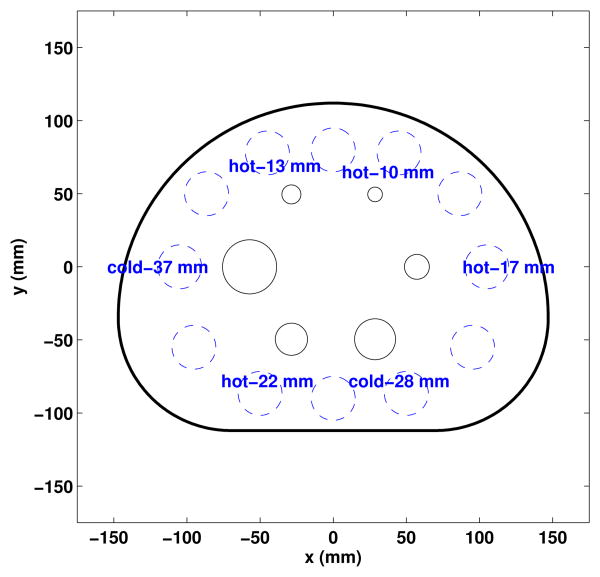
A NEMA phantom has been used to test the noise properties of different system models. Figure 6 shows the emission phantom which consists of 6 hot spheres located at the center of axial FOV. Four of six spheres were filled with ¹⁸F while the other two were filled with water with no activity. The activity ratio of the hot spheres to the warm background was 5:1. A total number of 54 million true coincidence events were generated to mimic a 3-minute clinical scan. For image reconstruction, we ran 10 OS-LMEM iterations with 10 subsets.

Figure 6.

The transverse view of a computer simulated NEMA phantom. The dashed-line shows the transverse view of the background ROI's.

First, images were reconstructed into an array of 300 × 300 × 89 with isotropic voxels of size 2.0 × 2.0 × 2.0 mm³. To evaluate the performance, we calculated the contrast recovery coefficient (CRC) versus background variability (BV). The CRC of the hot sphere is defined by

$$\text{CRC}(\%)=\frac{(\text{sphere mean})/(\text{background mean})-1}{\text{true contrast}-1}\times 100\%.$$ (8)

For the cold sphere, the CRC is defined by

$$\text{CRC}(\%)=1-(\text{sphere mean})/(\text{background mean})\times 100\%.$$ (9)

The background region of interest was selected on three different image slices. On each slice a total number of twelve disks each with a diameter of 30 mm were chosen (see figure 6). The three slices are located axially at: -1 cm, 0 mm and 1 cm, respectively. The BV is then calculated as the standard deviation of the means of 36 background ROIs.

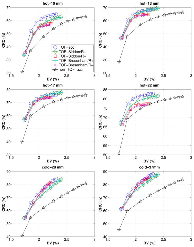
Figure 7 shows CRC versus BV curves for each sphere reconstructed using different system models. Overall, TOF outperforms non-TOF with less BV to achieve the same CRC. Among the TOF cases, difference can be clearly seen between TOF reconstructions with and without the image blurring matrix. Without the image blurring matrix, the maximum achievable CRC is substantially less than that with the image blurring matrix for all spheres. We also notice that the Bresenham's raytracer has nearly identical performance as the Siddon's raytracer, as the corresponding curves overlap very well.

Figure 7.

CRC versus BV for different spheres based on different system models. Here we used an image size 300 × 300 × 89 with voxel size 2 × 2 × 2 mm³. The first iteration starts at the left-bottom corner of each plot.

Figure 8 shows examples of reconstructed images with a matched BV value. Visually, both TOF-Siddon/R+ and TOF-Bresenham/R+ reconstructions look almost identical to that of TOF-acc. They all have better contrast than the non-TOF-acc image. Images reconstructed without an image blurring matrix (TOF-Siddon/R- and TOF-Bresenham/R-) appear to have different noise characteristics in the background region and lower contrast for hot spots.

Figure 8.

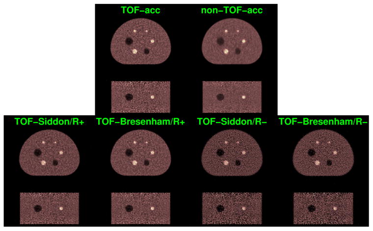
Reconstructed images of NEMA phantom based on different system models.

3.5. Effect of voxel size

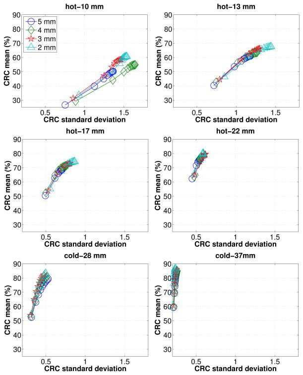
We studied the accuracy of the factored system matrix as a function of voxel size. We varied the transaxial voxel size from 2 mm to 5 mm. For each voxel size, a separate image blurring matrix was estimated using the same technique described previously. The same NEMA phantom shown in Figure 6 was used in the evaluation. A total number of 20 noisy realizations were generated, each of which has about 54 million true coincidence counts. All reconstruction were done with the TOF-Siddon/R+ model. Figure 9 shows the CRC mean vs. the CRC standard deviation as a function of iteration number for different voxel size. We see that higher CRC can be obtained by using a smaller voxel size. The difference between the CRC standard deviations of different voxel size is not statistically significant because of the small number of noisy realizations.

Figure 9.

Mean CRC versus standard deviation of CRC for each sphere based on the TOF-Siddon/R+ model. The first iteration starts at the left-bottom corner of each plot.

3.6. Correlation coefficients

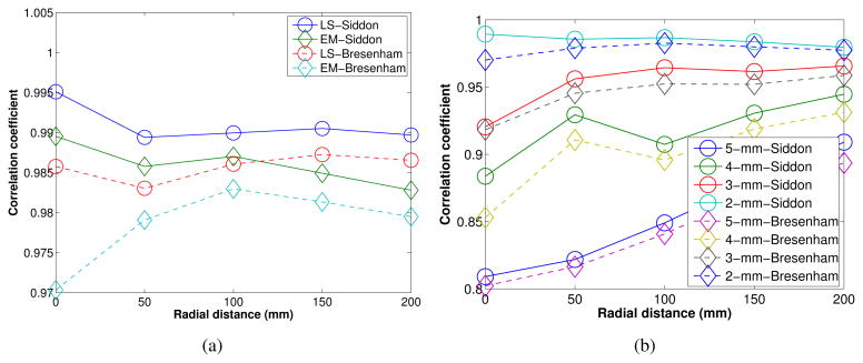
To compute the correlation coefficients given in (7), we simulated five point source scans using SimSET at five radial positions. The first point is located at the origin and the spacing between two adjacent locations is 50 mm. Each point source is a sphere of 0.5 mm in diameter. A water cylinder of 10 mm in diameter and 5 mm in height was used as the attenuation media. For each point, a total number for 620K true coincidence counts were generated. The data were then rebinned to 2D non-TOF sinogram and reconstructed using different geometrical projection matrices with voxel size ranging from 2 mm to 5 mm. When computing the CC in equation (7), we replace P_{TOF − acc}e_j by the simulated point source sinogram and r_j by the reconstructed point source image. Besides the nonnegativity constrained EM kernels that we estimated using (6), the least-square kernels mentioned in Section 2.4 were also estimated for comparison.

Figure 10(a) shows the resulting CC values as a function of radial position. As we can see, the LS kernel yields larger coefficients than the EM kernel does for a given geometrical projector. This indicates that the LS kernel outperforms the EM kernel in the sense of range condition. Figure 10(b) compares the CC for different voxel size. Clearly a smaller voxel size results in higher value of CC because a finer image sampling rate offers a higher degree of freedom that can capture more details of the underlying point spread function. This is consistent with the CRC curves shown in Figure 9. For a fixed voxel size, we see that the Siddon raytracer produces slightly higher CC than the Bresenham raytracer, but the difference is less than that caused by the change in voxel size.

Figure 10.

(a) A comparison of correlation coefficience for different point sources using different geometrical projection matrices together with different resolution kernels with (EM) and without (LS) nonnegativity constraint. (b) The change of CC as a function of voxel size for different geometrical projectors. ‘circle’: Siddon's raytracer, ‘diamond’: Bresenham's raytracer.

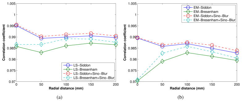
While sinogram blurring matrix is not compatible with the list-mode reconstruction, we evaluated its effect on model accuracy using the 2D Monte Carlo simulated sinogram. We computed the sinogram blurring matrix for each projector using the method we proposed in (Zhou and Qi 2011). Each point source was reconstructed using the geometrical projector together with the respective sinogram blurring matrix to obtain the image blurring kernel r_j. The point source reconstruction was performed using both the ML EM algorithm and LS estimation without the nonnegativity constraint. When computing the CC in equation (7), G̃_TOF was replaced by the product of the sinogram blurring matrix and the geometric projection matrix. The CC values are plotted as a function of radial distance in figure 11. Comparing with those shown in figure 10, we can see that the use of sinogram blurring matrix leads to a slight increase in the CC for both EM and LS kernels, although the improvement is greater for the Bresenham's raytracer.

Figure 11.

A comparison of model efficiency with and without additional sinogram domain blurring matrix: (a) CC using the LS kernel, and (b) CC using the EM kernel. The voxel size is 2-mm in all cases.

3.7. Computational cost

All source code was written in C++ and compiled using the GNU g++ compiler with option ‘O3’ added for performance optimization. The computational cost was measured on a computer running 64-bit Linux with two 2.4GHz Intel Xeon E5530 quad-core processors. On CPU we used OpenMP (http://www.openmp.org) for multithreaded computing. For comparison, we also implemented our method on GPU (GeForce GTX-480) with CUDA (NVIDIA 2008). The build-in atomic operations have been used to avoid the race condition encountered in backprojection.

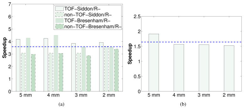
Table 2 compares the projection speed measured on the CPU and GPU for different image size using the same amount of list-mode data. The projection speeds were measured without the image blurring operation. On the CPU, the speedup associated with using a factored model is significant, which for the TOF case is more than a factor of ten. For the accurate model, TOF-acc has similar computational complexity as non-TOF-acc. This is because the TOF projection uses a precomputed non-TOF matrix which requires looping over all nonzeros regardless of the TOF window. However, for the factored model, the TOF projector is much faster than its non-TOF counterpart because the on-the-fly projector allows us to calculate TOF LOR based on the ±3σ truncation, which is much shorter than the non-TOF LOR. The on-the-fly projector can be further accelerated by using GPU. The speedup of the GPU-based projector over the CPU-based projector is plotted in figure 12(a). On average a GPU-based projector is 3.5 times faster than a CPU-based projector with 16 threads parallel computing. Figure 12(b) shows a comparison between the Siddon's raytracer and the Bresenham's raytracer. These quantities are based on the GPU implementation. We see that the Bresenham's raytracer is about 1.5 faster than the Siddon's raytracer. In table 3, we list the computation cost of the image blurring operation on the GPU. We also show the number of nonzeros in the estimated blurring matrices for various image sizes. We see that the time cost of the blurring operation is negligible. For the largest image size of 300 × 300 × 89, a forward and backward blurring operations take less than 0.2 second in total, which is insignificant as compared to the whole projection time.

Table 2.

Computation time of various projectors (unit in second). F.P.: forward projection, B.P.: backprojection, CPU: 16 threads (Intel Xeon E5530 quad-core processor), GPU: NVIDIA GTX480. The number of events is 54M.

image size	150 × 150 × 89			200 × 200 × 89			300 × 300 × 89
transaxial voxel size	4.0 mm × 4.0 mm			3.0 mm × 3.0 mm			2.0 mm × 2.0 mm
	CPU
	F.P.	B.P.	total	F.P.	B.P.	total	F.P.	B.P.	total
TOF-acc	196	250	446	311	383	694	625	787	1412
non-TOF-acc	151	358	509	258	491	749	514	838	1352
TOF-Siddon/R-	11	23	34	14	28	42	24	42	66
non-TOF-Siddon/R-	11	51	62	17	66	83	44	100	144
TOF-Bresenham/R-	3	20	23	5	20	25	9	30	39
non-TOF-Bresenham/R-	4	32	36	8	43	51	24	70	94
	GPU
	F.P.	B.P.	total	F.P.	B.P.	total	F.P.	B.P.	total
TOF-Siddon/R-	2.5	5.5	8	3.6	7.3	10.9	5.9	10.9	16.8
non-TOF-Siddon/R-	6.2	14	20.2	8.2	18.9	27.1	12	28	40
TOF-Bresenham/R-	1.6	3.5	5.1	2.3	4.7	7	3.8	7.2	11
non-TOF-Bresenham/R-	3.9	8.9	11.8	5.6	12.2	17.8	8.8	18.9	27.7

Figure 12.

(a) The speedup of GPU-based projector over CPU-based projector. (b) The speedup of Bresenham's raytracer over Siddon's raytracer. All dash lines indicate the average speedup factor.

Table 3.

The number of nonzeros in the image blurring matrices and the computation time (in millisecond) of the image blurring operation on the GPU for different image sizes.

image size	120 × 120 × 89	150 × 150 × 89	200 × 200 × 89	300 × 300 × 89
# of nonzeros in transaxial blurring matrix	116,888	216,076	548,424	1,988,372
# of nonzeros in axial blurring matrix	367	351	343	335
forward blurring (Rx) backward blurring (RTx)	3.6 ms 3.4 ms	7.5 ms 7.6 ms	21 ms 21 ms	95 ms 95 ms

4. Discussion and conclusion

We have studied a list-mode TOF PET image reconstruction using a factorized system model. The factored model primarily contains a geometrical projection matrix and an image blurring matrix. It is therefore well suitable for the list-mode data processing because there is no blurring operation in the sinogram space. The factored model allows us to use a simple geometrical projection matrix calculated on-the-fly, which can substantially reduce the computation time of the forward and back projection. The image blurring matrix is greatly important, which needs to be estimated based on the chosen geometrical projection matrix. In our simulation studies, we compared our factorization model to the accurate model. Quantitative analysis reveals that the performance of the proposed factorized model is comparable to the accurate one in terms of the spatial resolution and the noise properties while its reconstruction speed can be an order of magnitude faster than that of the non-factored model. The results also show that the Siddon's method is not the only choice for the on-the-fly calculation of geometrical projection. The Bresenham's method can be even faster while demonstrating the performance comparable to the Siddon's method.

To investigate model efficiency, we have proposed to compute the correlation coefficient to quantify the range condition as well as the linear dependence between the accurate model and the approximate model. Under this metric, we observed that the LS resolution model yields better performance than the EM resolution model for both geometrical projectors. We believe that this is because the LS kernel does not have nonnegativity constraint and hence is able to reduce the mismatch between the accurate model and the factored model. Therefore, it may also suggest that an unconstrained LS resolution kernel can potentially be a better choice than the non-negatively constrained EM resolution kernel. However, a resolution kernel with negative values may result in negative projections even for a nonnegative image, which can be problematic for the Poisson likelihood function. We plan to study this problem and develop a method to handle the LS resolution model in our future work. Using the CC criterion we compared factored models with and without an additional sinogram blurring matrix. We found that while the sinogram blurring matrix can improve the model accuracy, the improvement is relatively small. The same improvement can be also achieved by using smaller voxels in image reconstruction. Therefore, the proposed factored system matrix with only an image blurring matrix represents an efficient way for list-mode TOF PET reconstruction.

In current work, we only used analytical point source scans for the blurring matrix calculation. Such analytical image blurring kernel can be estimated for every voxel location independently but it is unable to model more complicated physical effects such as intercrystal scatter, as well as crystal mispositioning caused by electronic noise. Therefore, we plan to estimate another image space blurring matrix using real point source scans, and combine such a measurement-based blurring matrix with our analytical blurring matrix to further improve the model efficiency as well as the image reconstruction quality.

References

- Alessio A, Kinahan P, Lewellen T. Modeling and incorporation of system response functions in 3-D whole body PET. IEEE Transactions on Medical Imaging. 2006;25(7):828–837. doi: 10.1109/tmi.2006.873222. [DOI] [PubMed] [Google Scholar]
- Alessio AM, Stearns CW, Tong S, Ross SG, Kohlmyer S, Ganin A, Kinahan PE. Application and evaluation of a measured spatially variant system model for PET image reconstruction. IEEE Transactions on Medical Imaging. 2010;29(3):938–949. doi: 10.1109/TMI.2010.2040188. [DOI] [PMC free article] [PubMed] [Google Scholar]
- Bresenham J. Algorithm for computer control of a digital plotter. IBM Systems Journal. 1965;4(1):25–30. [Google Scholar]
- Byrne C. Iterative image reconstruction algorithms based on cross-entropy minimization. IEEE Transactions on Image Processing. 1993;2(1):96–103. doi: 10.1109/83.210869. [DOI] [PubMed] [Google Scholar]
- Cloquet C, Sureau F, Defrise M, Simaeys G, Trotta N, Goldman S. Non-gaussian space-variant resolution modeling for list-mode reconstruction. Physics in Medicine and Biology. 2010;55(17):5045–5066. doi: 10.1088/0031-9155/55/17/011. [DOI] [PubMed] [Google Scholar]
- Cui J, Pratx G, Levin C. Fully 3D list-mode time-of-flight PET image reconstruction on GPUs using CUDA. Medical physics. 2011;38(12):6775–6789. doi: 10.1118/1.3661998. [DOI] [PubMed] [Google Scholar]
- Hu Z, Wang W, Gualtieri E, Parma M, Walsh E, Sebok D, Hsieh Y, Tung C, Griesmer J, Kolthammer J, Popescu L, Werner M, Karp J, Bucur A, van Leeuwen J, Gagnon D. Dynamic load balancing on distributed listmode time-of-flight image reconstruction. Nuclear Science Symposium Conference Record, 2006. IEEE; 2006. pp. 3392–3396. [Google Scholar]
- Huesman R, Klein G, Moses W, Qi J, Reutter B, Virador P. List-mode maximum-likelihood reconstruction applied to positron emission mammography (PEM) with irregular sampling. IEEE Transactions on Medical Imaging. 2000;19(5):532–537. doi: 10.1109/42.870263. [DOI] [PubMed] [Google Scholar]
- Lewellen T, Harrison R, Vannoy S. The simSET program. In: Ljungberg M, Strand S, King M, editors. Monte Carlo Calculations in Nuclear Medicine. Philadelphia, PA: Inst Phys; 1998. [Google Scholar]
- Mumcuoglu E, Leahy R, Cherry S, Hoffman E. Accurate geometric and physical response modeling for statistical image reconstruction in high resolution PET. 1996 IEEE Nuclear Science Symposium, Conference Record; 1996. pp. 1569–1573. vol. 3. [Google Scholar]
- NVIDIA. CUDA. 2008 available at: http://www.nvidia.com/object/cuda_home_new.html.
- Panin V, Kehren F, Michel C, Casey M. Fully 3-D PET reconstruction with system matrix derived from point source measurements. IEEE Transactions on Medical Imaging. 2006;25(7):907–921. doi: 10.1109/tmi.2006.876171. [DOI] [PubMed] [Google Scholar]
- Popescu L, Matej S, Lewitt R. Iterative image reconstruction using geometrically ordered subsets with list-mode data. Nuclear Science Symposium Conference Record, 2004 IEEE; 2004. pp. 3536–3540. [Google Scholar]
- Pratx G, Levin C. Online detector response calculations for high-resolution PET image reconstruction. Physics in Medicine and Biology. 2011;56(13):4023. doi: 10.1088/0031-9155/56/13/018. [DOI] [PMC free article] [PubMed] [Google Scholar]
- Pratx G, Surti S, Levin C. Fast list-mode reconstruction for time-of-flight PET using graphics hardware. IEEE Transactions on Nuclear Science. 2011;58(1):105–109. [Google Scholar]
- Qi J, Leahy R, Cherry S, Chatziioannou A, Farquhar T. High-resolution 3D Bayesian image reconstruction using the microPET small-animal scanner. Physics in Medicine and Biology. 1998;43(4):1001–1013. doi: 10.1088/0031-9155/43/4/027. [DOI] [PubMed] [Google Scholar]
- Rahmim A, Qi J, Sossi V. Resolution modeling in PET imaging: Theory, practice, benefits, and pitfalls. Medical Physics. 2013;40(6):064301. doi: 10.1118/1.4800806. [DOI] [PMC free article] [PubMed] [Google Scholar]
- Rapisarda E, Bettinardi V, Thielemans K, Gilardi M. Image-based point spread function implementation in a fully 3D OSEM reconstruction algorithm for PET. Physics in Medicine and Biology. 2010;55(14):4131–4151. doi: 10.1088/0031-9155/55/14/012. [DOI] [PubMed] [Google Scholar]
- Shepp L, Vardi Y. Maximum likelihood reconstruction for emission tomography. IEEE Transactions on Medical Imaging. 1982;1(2):113–122. doi: 10.1109/TMI.1982.4307558. [DOI] [PubMed] [Google Scholar]
- Siddon R. Fast calculation of the exact radiological path for a three-dimensional CT array. Medical physics. 1985;12(2):252–255. doi: 10.1118/1.595715. [DOI] [PubMed] [Google Scholar]
- Stute S, Comtat C. Practical considerations for image-based PSF and blobs reconstruction in PET. Physics in Medicine and Biology. 2013;58(11):3849–3870. doi: 10.1088/0031-9155/58/11/3849. [DOI] [PubMed] [Google Scholar]
- Sureau F, Reader A, Comtat C, Leroy C, Ribeiro M, Buvat I, Trebossen R. Impact of image-space resolution modeling for studies with the high-resolution research tomograph. Journal of Nuclear Medicine. 2008;49(6):1000–1008. doi: 10.2967/jnumed.107.045351. [DOI] [PubMed] [Google Scholar]
- Surti S, Kuhn A, Werner M, Perkins A, Kolthammer J, Karp J. Performance of philips gemini TF PET/CT scanner with special consideration for its time-of-flight imaging capabilities. Journal of Nuclear Medicine. 2007;48(3):471–480. [PubMed] [Google Scholar]
- Tohme M, Qi J. Experimental evaluation of system models for PET with block detectors. IEEE Nuclear Science Symposium Conference Record, 2006; 2006. pp. 2778–2782. [Google Scholar]
- Tohme M, Qi J. Iterative image reconstruction for positron emission tomography based on a detector response function estimated from point source measurements. Physics in Medicine and Biology. 2009;54(12):3709–3725. doi: 10.1088/0031-9155/54/12/007. [DOI] [PMC free article] [PubMed] [Google Scholar]
- Wang W, Hu Z, Gualtieri E, Parma M, Walsh E, Sebok D, Hsieh YL, Tung CH, Song X, Griesmer J, Kolthammer J, Popescu L, Werner M, Karp J, Gagnon D. Systematic and distributed time-of-flight list mode pet reconstruction. Nuclear Science Symposium Conference Record, 2006. IEEE; 2006. pp. 1715–1722. [Google Scholar]
- Zhou J, Qi J. Fast and efficient fully 3D PET image reconstruction using sparse system matrix factorization with GPU acceleration. Physics in Medicine and Biology. 2011;56(20):6739–6758. doi: 10.1088/0031-9155/56/20/015. [DOI] [PMC free article] [PubMed] [Google Scholar]