

Abstract
This work studies the problem of privacy-preserving classification – namely, learning a classifier from sensitive data while preserving the privacy of individuals in the training set. In particular, the learning algorithm is required in this problem to guarantee differential privacy, a very strong notion of privacy that has gained significant attention in recent years.
A natural question to ask is: what is the sample requirement of a learning algorithm that guarantees a certain level of privacy and accuracy? We address this question in the context of learning with infinite hypothesis classes when the data is drawn from a continuous distribution. We first show that even for very simple hypothesis classes, any algorithm that uses a finite number of examples and guarantees differential privacy must fail to return an accurate classifier for at least some unlabeled data distributions. This result is unlike the case with either finite hypothesis classes or discrete data domains, in which distribution-free private learning is possible, as previously shown by Kasiviswanathan et al. (2008).
We then consider two approaches to differentially private learning that get around this lower bound. The first approach is to use prior knowledge about the unlabeled data distribution in the form of a reference distribution
 chosen independently of the sensitive data. Given such a reference
, we provide an upper bound on the sample requirement that depends (among other things) on a measure of closeness between
and the unlabeled data distribution. Our upper bound applies to the non-realizable as well as the realizable case. The second approach is to relax the privacy requirement, by requiring only label-privacy – namely, that the only labels (and not the unlabeled parts of the examples) be considered sensitive information. An upper bound on the sample requirement of learning with label privacy was shown by Chaudhuri et al. (2006); in this work, we show a lower bound.
chosen independently of the sensitive data. Given such a reference
, we provide an upper bound on the sample requirement that depends (among other things) on a measure of closeness between
and the unlabeled data distribution. Our upper bound applies to the non-realizable as well as the realizable case. The second approach is to relax the privacy requirement, by requiring only label-privacy – namely, that the only labels (and not the unlabeled parts of the examples) be considered sensitive information. An upper bound on the sample requirement of learning with label privacy was shown by Chaudhuri et al. (2006); in this work, we show a lower bound.
Keywords: Privacy, generalization, PAC-learning
1. Introduction
As increasing amounts of personal data is collected, stored and mined by companies and government agencies, the question of how to learn from sensitive datasets while still maintaining the privacy of individuals in the data has become very important. Over the last few years, the notion of differential privacy (Dwork et al., 2006) has received a significant amount of attention, and has become the de facto standard for privacy-preserving computation. In this paper, we study the problem of learning a classifier from a dataset, while simultaneously guaranteeing differential privacy of the training data.
The key issue in differentially-private computation is that given a certain amount of resources, there is usually a tradeoff between privacy and utility. In classification, a natural measure of utility is the classification accuracy, and data is a scarce resource. Thus, a key question in differentially-private learning is: how many examples does a learning algorithm need to guarantee a certain level of privacy and accuracy? In this paper, we study this question from an information-theoretic perspective – namely, we are concerned with the sample complexity, and not the computational complexity of the learner.
This question was first considered by Kasiviswanathan et al. (2008), who studied the case of finite hypothesis classes, as well as the case of discrete data domains. They showed that in these two cases, one can obtain any given privacy guarantee and generalization error, regardless of the unlabeled data distribution with a modest increase in the worst-case sample requirement.
In this paper, we consider the sample complexity of differentially private learning in the context of infinite hypothesis classes on continuous data distributions. This is a very general class of learning problems, and includes many popular machine-learning tasks such as learning linear classifiers when the examples have real-valued features, which cannot be modeled by finite hypothesis classes or hypothesis classes over discrete data domains.
Surprisingly, we show that the results of Kasiviswanathan et al. (2008) do not extend to infinite hypothesis classes on continuous data distributions. As an example, consider the class of thresholds on the unit interval. This simple learning problem has VC dimension 1, and thus for all unlabeled data distributions, it can be learnt (non-privately) with error ε given at most examples1. We show that even for this very simple hypothesis class, any algorithm that uses a bounded number of examples and guarantees differential privacy must fail to return an accurate classifier for at least some unlabeled data distributions.
The key intuition behind our proof is that if most of the unlabeled data is concentrated in a small region around the best classifier, then, even slightly perturbing the best classifier will result in a large classification error. As the process of ensuring differential privacy necessarily involves some perturbation – see, for example, Dwork et al. (2006), unless the algorithm has some prior public knowledge about the data distribution, the number of samples required to learn privately grows with growing concentration of the data around the best classifier.
How can we then learn privately in infinite hypothesis classes over continuous data distributions? One approach is to use some prior information about the data distribution that is known independently of the sensitive data. Another approach is to relax the privacy requirements. In this paper, we examine both approaches.
First, we consider the case when the learner has access to some prior information on the unlabeled data. In particular, the learner knows a reference distribution
that is close to the unlabeled data distribution. Similar assumptions are common in Bayesian learning, and PAC-Bayes style bounds have also been studied in the learning theory literature, for example, by McAllester (1998).
Under this assumption, we provide an algorithm for learning with α-privacy, excess generalization error ε, and confidence 1 − δ, using
samples. Here α is a privacy parameter (where, lower α implies a stronger privacy guarantee),
is the reference distribution, d is the doubling dimension of its disagreement metric (Bshouty et al., 2009), and κ is a smoothness parameter that we define. The quantity d measures the complexity of the hypothesis class with respect to
(see (Bshouty et al., 2009) for a discussion), and we assume that it is finite. The smoothness parameter measures how close the unlabeled data distribution is to
(smaller κ means closer), and is motivated by notions of closeness used in Dasgupta (2005) and Freund et al. (1997). Thus the sample requirement of our algorithm grows with increasing distance between
and the unlabeled data distribution. Our algorithm works in the non-realizable case, that is, when no hypothesis in the class has zero error; using standard techniques, a slightly better bound of
can be obtained in the realizable setting. However, like the results of Kasiviswanathan et al. (2008), our algorithm is computationally inefficient in general.
is the doubling dimension of its disagreement metric (Bshouty et al., 2009), and κ is a smoothness parameter that we define. The quantity d measures the complexity of the hypothesis class with respect to
(see (Bshouty et al., 2009) for a discussion), and we assume that it is finite. The smoothness parameter measures how close the unlabeled data distribution is to
(smaller κ means closer), and is motivated by notions of closeness used in Dasgupta (2005) and Freund et al. (1997). Thus the sample requirement of our algorithm grows with increasing distance between
and the unlabeled data distribution. Our algorithm works in the non-realizable case, that is, when no hypothesis in the class has zero error; using standard techniques, a slightly better bound of
can be obtained in the realizable setting. However, like the results of Kasiviswanathan et al. (2008), our algorithm is computationally inefficient in general.
The main difficulty in reducing the differentially-private learning algorithms of Kasiviswanathan et al. (2008) to infinite hypothesis classes on continuous data distributions is in finding a suitable finite cover of the class with respect to the unlabeled data. This issue is specific to our particular problem: for non-private learning, a finite cover can always be computed based on the (sensitive) data, and for finite hypothesis classes, the entire class is a cover. The main insight behind our upper bound is that when the unlabeled distribution
 is close to the reference distribution
, then a cover of
is also a possibly coarser cover of
. Since one can compute a private cover of
independent of the sensitive data, we simply compute a finer cover of
, and learn over this fine cover using standard techniques such as the exponential mechanism (McSherry and Talwar, 2007).
is close to the reference distribution
, then a cover of
is also a possibly coarser cover of
. Since one can compute a private cover of
independent of the sensitive data, we simply compute a finer cover of
, and learn over this fine cover using standard techniques such as the exponential mechanism (McSherry and Talwar, 2007).
Next we relax the privacy requirement by requiring only label privacy. In other words, we assume that the unlabeled part of the examples are not sensitive, and the only private information is the labels. This setting was considered by Chaudhuri et al. (2006). An example when this may be applicable is in predicting income from public demographic information. Here, while the label (income) is private, the demographic information of individuals, such as education, gender, and age may be public.
In this case, we provide lower bounds to characterize the sample requirement of label-private learning. We show two results, based on the value of α and ε. For small ε and α (that is, for high privacy and accuracy) we show that any learning algorithm for a given hypothesis class that guarantees α-label privacy and ε accuracy necessarily requires at least examples. Here d is the doubling dimension of the disagreement metric at a certain scale, and is a measure of the complexity of the hypothesis class on the unlabeled data distribution. This bound holds when the hypothesis class has finite VC dimension. For larger α and ε, our bounds are weaker but more general; we show a lower bound of on the sample requirement that holds for any α and ε, and do not require the VC dimension of the hypothesis class to be finite. Here d′ is the doubling dimension of the disagreement metric at a certain scale.
The main idea behind our stronger label privacy lower bounds is to show that differentially private learning algorithms necessarily perform poorly when there is a large set of hypotheses such that every pair in the set labels approximately 1/α examples differently. We then show that such large sets can be constructed when the doubling dimension of the disagreement metric of the hypothesis class with respect to the data distribution is high.
How do these results fit into the context of non-private learning? For non-private learning, sample requirement bounds based on the doubling dimension of the disagreement metric has been extensively studied by (Bshouty et al., 2009); in the realizable case, they show an upper bound of for learning with accuracy ε, where d̄ is again the doubling dimension of the disagreement metric at a certain scale. These bounds are incomparable to ours in general, as the doubling dimensions in the two bounds are with respect to different scales; however, we can compare them for hypothesis classes and data distributions for which the doubling dimension of the disagreement metric is equal at all scales. An example is learning half spaces with respect to the uniform distribution on the sphere. For such problems, on the upper bound side, we need a factor of times more examples to learn with α-privacy. On the other hand, our lower bounds indicate that for small α and ε, even if we only want α-label privacy, the sample requirement can be as much as a factor of more than the upper bound for non-private learning.
Finally, one may be tempted to think that we can always discretize a data domain or a hypothesis class, and therefore in practice we are likely to only learn finite hypothesis classes or over discrete data domains. However, there are several issues with such discretization. First, if we discretize either the hypothesis class or the data, then the sample requirement of differentially private learning algorithms will grow as the discretization grows finer, instead of depending on intrinsic properties of the problem. Second, as our α-privacy lower bound example shows, indiscriminate discretization without prior knowledge of the data can drastically degrade the performance of the best classifier in a class. Finally, infinite hypothesis classes and continuous data domains provide a natural abstraction for designing many machine learning algorithms, such as those based on convex optimization or differential geometry. Understanding the limitations of differentially private learning on such hypothesis classes and data domains is useful in designing differentially private approximations to these algorithms.
The rest of our paper is organized as follows. In Section 2, we define some preliminary notation, and explain our privacy model. In Section 3, we present our α-privacy lower bound. Our α-privacy upper bound is provided in Section 4. In Section 5, we provide some lower bounds on the sample requirement of learning with α-label privacy. Finally, the proofs of most of our results are in the appendix.
1.1. Related work
The work most related to ours is Kasiviswanathan et al. (2008), Blum et al. (2008) and Beimel et al. (2010), each of which deals with either finite hypothesis classes or discrete data domains.
Kasiviswanathan et al. (2008) initiated the study of the sample requirement of differentially-private learning. They provided a (computationally inefficient) α-private algorithm that learns any finite hypothesis class
 with error at most ε using at most
examples in the realizable case. For the non-realizable case, they provided an algorithm with a sample requirement of
. Moreover, using a result from Blum et al. (2008), they provided a computationally inefficient α-private algorithm that learns a hypothesis class with VC-dimension V and data dimension n with at most
examples, provided the data domain is {−1, 1}n. The latter result does not apply when the data is drawn from a continuous distribution; moreover, their results cannot be directly extended to the continuous case.
with error at most ε using at most
examples in the realizable case. For the non-realizable case, they provided an algorithm with a sample requirement of
. Moreover, using a result from Blum et al. (2008), they provided a computationally inefficient α-private algorithm that learns a hypothesis class with VC-dimension V and data dimension n with at most
examples, provided the data domain is {−1, 1}n. The latter result does not apply when the data is drawn from a continuous distribution; moreover, their results cannot be directly extended to the continuous case.
The first work to study lower bounds on the sample requirement of differentially private learning was Beimel et al. (2010). They show that any α-private algorithm that selects a hypothesis from a specific set Cε requires at least Ω̃(log(|Cε|)/α) samples to achieve error ε. Here Cε is an ε-cover as well as an ε-packing of the hypothesis class
with respect to every distribution over the discrete data domain. They also show an upper bound of Õ(log(|Cε|)/(αε)). Such a cover Cε does not exist for continuous data domains; as a result their upper bounds do not apply to our setting. Moreover, unlike our lower bounds, their lower bound only applies to algorithms of a specific form (namely, those that output a hypothesis in Cε), and it also does not apply when we only require the labels to be private.
For the setting of label privacy, Chaudhuri et al. (2006) show an upper bound for PAC-learning in terms of the VC dimension of the hypothesis class. We show a result very similar to theirs in the appendix for completeness, and we show lower bounds for learning with label-privacy which indicate that their bounds are almost tight, in terms of the dependence on α and ε.
Zhou et al. (2009) study some issues in defining differential privacy when dealing with continuous outcomes; however, they do not consider the question of learning classifiers on such data.
Finally, a lot of our work uses tools from the theory of generalization bounds. In particular, some of our upper and lower bounds are inspired by Bshouty et al. (2009), which bounds the sample complexity of (non-private) classification in terms of the doubling dimension of the disagreement metric.
Other related work on privacy
The issue of privacy in data analysis of sensitive information has long been a source of problems for curators of such data, and much of this is due to the realization that many simple and intuitive mechanisms designed to protect privacy are simply ineffective. For instance, the work of Narayanan and Shmatikov (2008) showed that an anonymized dataset released by Netflix revealed enough information so that an adversary, by knowing just a few of the movies rated by a particular user, would be able to uniquely identify such a user in the data set and determine all of his movie ratings. Similar attacks have been demonstrated on private data in other domains as well including social networks (Backstrom et al., 2007) and search engine query logs (Jones et al., 2007). Even releasing coarse statistics without proper privacy safeguards can be problematic. This was recently shown by Wang et al. (2009) in the context of genetic data, where a correlation matrix of genetic markers compiled from a group of individuals contained enough clues to uniquely pinpoint individuals in the dataset and learn of their private information, such as whether or not they had certain diseases.
In order to reason about privacy guarantees (or lack thereof), we need a formal definition of what it means to preserve privacy. In our work, we adopt the notion of differential privacy due to Dwork et al. (2006), which has over the last few years gained much popularity. Differential privacy is known to be a very strong notion of privacy: it has strong semantic guarantees (Kasiviswanathan and Smith, 2008) and is resistant to attacks that many earlier privacy definitions are susceptible to (Ganta et al., 2008b).
There has been a significant amount of work on differential privacy applied to a wide variety of data analysis tasks (Dwork et al., 2006; Chaudhuri and Mishra, 2006; Nissim et al., 2007; Barak et al., 2007; McSherry and Mironov, 2009). Some work that is relevant to ours include Blum et al. (2008), which provides a general method for publishing datasets on discrete data domains while preserving differential privacy so that the answers to queries from a function class with bounded VC dimension will be approximately preserved after the applying the sanitization procedure. More work on this line includes Roth (2010) and Gupta et al. (2011). A number of learning algorithms have also been suitably modified to guarantee differential privacy. For instance, both the classes of statistical query algorithms and the class of methods based on L2-regularized empirical risk minimization with certain types of convex losses can be made differentially private (Blum et al., 2005; Chaudhuri et al., 2011).
There has also been some prior work on providing lower bounds on the loss of accuracy that any differentially private mechanism would suffer; much of this work is in the context of releasing answers to some a of queries made on a database of n individuals. The first such work is by (Blum et al., 2008), which shows that no differentially private mechanism can hope to release with a certain amount of accuracy the answer to a number of median queries when the data lies on a real line. This result is similar in spirit to our Theorem 5, but applies to a much harder problem, namely data release. Other relevant work includes (Hardt and Talwar, 2010), which uses a packing argument similar to ours to provide a lower bound on the amount of noise any differentially private mechanism needs to add to the answer to k linear queries on a database of n people.
There has also been a significant amount of prior work on privacy-preserving data mining (Agrawal and Srikant, 2000; Evfimievski et al., 2003; Sweeney, 2002; Machanavajjhala et al., 2006), which spans several communities and uses privacy models other than differential privacy. Many of the models used have been shown to be susceptible to various attacks, such as composition attacks, where the adversary has some amount of prior knowledge (Ganta et al., 2008a). An alternative line of privacy work is in the Secure Multiparty Computation setting due to Yao (1982), where the sensitive data is split across several adversarial databases, and the goal is to compute a function on the union of these databases. This is in contrast with our setting, where a single centralized algorithm can access the entire dataset.
2. Preliminaries
2.1. Privacy model
We use the differential privacy model of Dwork et al. (2006). In this model, a private database DB ⊆
 consists of m sensitive entries from a domain
; each entry in DB is a record about an individual (e.g., their medical history) that one wishes to keep private.
consists of m sensitive entries from a domain
; each entry in DB is a record about an individual (e.g., their medical history) that one wishes to keep private.
The database DB is accessed by users through a sanitizer M. The sanitizer, a randomized algorithm, is said to preserve differential privacy if the value of any one individual in the database does not significantly alter the output distribution of M.
Definition 1
A randomized mechanism M guarantees α-differential privacy if, for all databases DB1 and DB2 that differ by the value of at most one individual, and for every set G of possible outputs of M,
We emphasize that the probability in the definition above is only with respect to the internal randomization of the algorithm; it is independent of all other random sources, including any that may have generated the values of the input database.
Differential privacy is a strong notion of privacy (Dwork et al., 2006; Kasiviswanathan and Smith, 2008; Ganta et al., 2008b). In particular, if a sanitizer M ensures α-differential privacy, then, an adversary who knows the private values of all the individuals in the database except for one and has arbitrary prior knowledge about the value of the last individual, cannot gain additional confidence about the private value of the last individual by observing the output of a differentially private sanitizer. The level of privacy is controlled by α, where a lower value of α implies a stronger guarantee of privacy.
2.2. Learning model
We consider a standard probabilistic learning model for binary classification. Let
 be a distribution over
 × {±1}, where
is the data domain and {±1} are the possible labels. We use
to denote the marginal of
over the data domain
. The classification error of a hypothesis h:
→ {±1} with respect to a data distibution
is
× {±1}, where
is the data domain and {±1} are the possible labels. We use
to denote the marginal of
over the data domain
. The classification error of a hypothesis h:
→ {±1} with respect to a data distibution
is
We denote by S ~
 an i.i.d. draw of m labeled examples S = {(x1, y1), …, (xm, ym)} ⊆
×{±1} from the distribution
. This process can equivalently be seen as drawing an unlabeled sample X:= {x1, …, xm} from the marginal
, and then, for each x ∈ X, drawing the corresponding label y from the induced conditional distribution.
an i.i.d. draw of m labeled examples S = {(x1, y1), …, (xm, ym)} ⊆
×{±1} from the distribution
. This process can equivalently be seen as drawing an unlabeled sample X:= {x1, …, xm} from the marginal
, and then, for each x ∈ X, drawing the corresponding label y from the induced conditional distribution.
A learning algorithm is given as input a set of m labeled examples S ~
, a target accuracy parameter ε ∈ (0, 1), and target confidence parameter δ ∈ (0, 1). Its goal is to return a hypothesis h:
→ {±1} such that its excess generalization error with respect to a specified hypothesis class
is at most ε with probability at least 1 − δ over the random choice of the sample S ~
, as well as any internal randomness of the algorithm.
We also occasionally adopt the realizable assumption (with respect to
). The realizable assumption states that there exists some h* ∈
such that Pr(x,y)~
 [h*(x) ≠ y] = 0. In this case, the excess generalization error of a hypothesis h is simply its classification error. Without the realizable assumption, there may be no classifier in the hypothesis class
with zero classification error, and we refer to this as the non-realizable case.
[h*(x) ≠ y] = 0. In this case, the excess generalization error of a hypothesis h is simply its classification error. Without the realizable assumption, there may be no classifier in the hypothesis class
with zero classification error, and we refer to this as the non-realizable case.
2.3. Privacy-preserving classification
In privacy-preserving classification, we assume that the database is a training dataset drawn in an i.i.d manner from some data distribution
, and that the sanitization mechanism is a learning algorithm that outputs a classifier based on the training data. In this paper, we consider two possible privacy requirements on our learning algorithms.
Definition 2
A randomized learning algorithm
 guarantees α-label privacy (
is α-label private) if, for any two datasets S1 = {(x1, y1), …, (xm−1, ym−1), (xm, ym)} and
differing in at most one label
, and any set of outputs G of
,
guarantees α-label privacy (
is α-label private) if, for any two datasets S1 = {(x1, y1), …, (xm−1, ym−1), (xm, ym)} and
differing in at most one label
, and any set of outputs G of
,
Definition 3
A randomized learning algorithm
guarantees α-privacy (
is α-private) if, for any two datasets S1 = {(x1, y1), …, (xm−1, ym−1), (xm, ym)} and
differing in at most one example (
), and any set of outputs G of
,
Note that if the input dataset S is a random variable, then for any value S′ ⊆
× {±1} in the range of S, the conditional probability distribution of
(S) | S = S′ is determined only by the algorithm
and the value S′; it is independent of the distribution of the random variable S. Therefore, for instance,
for any S′ ⊆
× {±1} and any set of outputs G.
The difference between the two notions of privacy is that for α-label privacy, the two databases can differ only in the label of one example; whereas for α-privacy, the two databases differ can differ in a complete example (both labeled and unlabeled parts). Thus, α-label privacy only ensures the privacy of the label component of each example; it makes no guarantees about the unlabeled part. If a classification algorithm guarantees α-privacy, then it also guarantees α-label privacy. Thus α-label privacy is a weaker notion of privacy than α-privacy.
The notion of label privacy was also considered by Chaudhuri et al. (2006), who provided an algorithm for learning with label privacy. For strict privacy, one would require the learning algorithm to guarantee α-privacy; however, label privacy may also be an useful notion. For example, if the data x represents public demographic information (e.g., age, zip code, education), while the label y represents income level, an individual may consider the label to be private but may not mind if others can infer her demographic information (which could be relatively public already) by her inclusion in the database.
Thus, the goal of a α-private (resp. α-label private) learning algorithm is as follows. Given a dataset S of size m, a privacy parameter α, a target accuracy ε, and a target confidence parameter δ:
guarantee α-privacy (resp. α-label privacy) of the training dataset S;
- with probability at least 1 − δ over both the random choice of S ~ and the internal randomness of the algorithm, return a hypothesis h:
→ {±1} with excess generalization error
2.4. Additional definitions and notation
We now present some additional essential definitions and notation.
Metric spaces, doubling dimension, covers, and packings
A metric space (
, ρ) is a tuple, where
is a set of elements, and ρ is a distance function from
×
to {0} ∪ ℝ+. Let (
, ρ) be any arbitrary metric space. For any z ∈
and r > 0, let B(z, r) = {z′ ∈
: ρ(z, z′) ≤ r} denote the ball centered at z of radius r.
The diameter of (
, ρ) is sup{ρ(z, z′): z, z′ ∈
}, the longest distance in the space. An ε-cover of (
, ρ) is a set C ⊆
such that for all z ∈
, there exists some z′ ∈ C such that ρ(z, z′) ≤ ε. An ε-packing of (
, ρ) is a set P ⊆
such that ρ(z, z′) > ε for all distinct z, z′ ∈ P. Let
 (
, ρ) denote the size of the smallest ε-cover of (
, ρ).
(
, ρ) denote the size of the smallest ε-cover of (
, ρ).
We define the doubling dimension of (
, ρ) at scale ε, denoted as ddimε(
, ρ), as the smallest number d such that each ball B(z, ε) ⊆
of radius ε can be covered by at most ⌊2d⌋ balls of radius ε/2, i.e. there exists z1, …, z⌊2d⌋ ∈
such that B(z, ε) ⊆ B(z1, ε/2) ∪ … ∪ B(z⌊2d⌋, ε/2). Notice that ddimε(
, ρ) may increase or decrease with ε. The doubling dimension of (
, ρ) is sup{ddimr(
, ρ): r > 0}.
Disagreement metrics
The disagreement metric of a hypothesis class
with respect to a data distribution
over
is the metric (
, ρ ), where ρ is the following distance function:
The empirical disagreement metric of a hypothesis class
with respect to a data distribution
over
is the metric (
, ρX), where ρX is the following distance function:
The disagreement metric (or empirical disagreement metric) is the proportion of unlabeled examples on which h and h′ disagree with respect to
(or the uniform distribution over X). We use the notation B (h, r) to denote the ball centered at h of radius r with respect to ρ, and BX(h, r) to denote the ball centered at h of radius r with respect to ρX.
Datasets and empirical error
For an unlabeled dataset X ⊆
and a hypothesis h:
→ {±1}, we denote by SX,h:= {(x, h(x)): x ∈ X} the labeled dataset induced by labeling X with h. The empirical error of a hypothesis h:
→ {±1} with respect to a labeled dataset S ⊆
× {±1} is err(h, S):= (1/|S|)Σ(x,y) ∈S
 [h(x) ≠ y] the average number of mistakes that h makes on S; note that ρX(h, SX,h′) = err(h, SX,h′). Finally, we informally use the Õ(·) notation to hide log(1/δ) factors, as well as factors that are logarithmic in those that do appear.
3. Lower bounds for learning with α-privacy
In this section, we show a lower bound on the sample requirement of learning with α-privacy. In particular, we show an example that illustrates that when the data is drawn from a continuous distribution, for any M, all α-private algorithms that are supplied with at most M examples fail to output a good classifier for at least one unlabeled data distribution.
Our example hypothesis class is the class of thresholds on [0, 1]. This simple class has VC dimension 1, and thus can be learnt non-privately with classification error ε given only Õ(1/ε) examples, regardless of the unlabeled data distribution. However, Theorem 5 shows that even in the realizable case, for every α-private algorithm that is given a bounded number of examples, there is at least one unlabeled data distribution on which the learning algorithm produces a classifier with error , with probability at least 1/2 over its own random coins.
The key intuition behind our example is that if most of the unlabeled data is concentrated in a small region around the best classifier, then, even slightly perturbing the best classifier will result in a large classification error. As the process of ensuring differential privacy necessarily involves some perturbation, unless the algorithm has some prior public knowledge about the data distribution, the number of samples required to learn privately grows with growing concentration of the data around the best classifier. As illustrated by our theorem, this problem is not alleviated if the support of the unlabeled distribution is known; even if the data distribution has large support, a large fraction of the data can still lie in a region close to the best classifier.
Before we describe our example in detail, we first need a definition.
Definition 4
The class of thresholds on the unit interval is the class of functions hw: [0, 1] → {−1, 1} such that:
Theorem 5
Let M > 2 be any number, and let
be the class of thresholds on the unit interval [0, 1]. For any α-private algorithm A that outputs a hypothesis h ∈
, there exists a distribution
on labeled examples with the following properties:
There exists a threshold h* ∈
with classification error 0 with respect to
.For all samples S of size m ≤ M drawn from
, with probability at least 1/2 over the random coins of A, the hypothesis output by A(S) has classification error at least
with respect to
.The marginal
of
over the unlabeled data has support [0, 1].
Proof
Let
, and let
denote the uniform distribution over [0, 1]. Let Z = {η, 2η, …, Kη}, where K = ⌊1/η⌋ − 1. We let Gz = [z − η/3, z + η/3] for z ∈ Z, and let
 ⊂
be the subset of thresholds:
= {hτ|τ ∈ Gz}. We note that Gz ⊆ [0, 1] for all z ∈ Z.
⊂
be the subset of thresholds:
= {hτ|τ ∈ Gz}. We note that Gz ⊆ [0, 1] for all z ∈ Z.
For each z ∈ Z, we define a distribution
 over labeled examples as follows. First, we describe the marginal
 of
over the unlabeled data. A sample from
is drawn as follows. With probability
, x is drawn from
; with probability
, it is drawn from uniformly from Gz. Now, an unlabeled example x drawn from
is labeled positive if x ≥ z, and negative otherwise. We observe that for every such distribution
, there exists a threshold, namely, hz that has classification error 0; in addition, the support of
is [0, 1]. Moreover, there are
such distributions
in all, and
.
of
over the unlabeled data. A sample from
is drawn as follows. With probability
, x is drawn from
; with probability
, it is drawn from uniformly from Gz. Now, an unlabeled example x drawn from
is labeled positive if x ≥ z, and negative otherwise. We observe that for every such distribution
, there exists a threshold, namely, hz that has classification error 0; in addition, the support of
is [0, 1]. Moreover, there are
such distributions
in all, and
.
We say that an α-private algorithm A succeeds on a sample S with respect to a distribution
if with probability
over the random coins of A, the hypothesis output by A(S) has classification error
over
.
Suppose for the sake of contradiction that there exists an α-private algorithm A* such that for all distributions
, there is at least one sample S of size ≤ M drawn from
such that A* succeeds on S with respect to
. Then, for all z ∈ Z, and for all
, there exists a sample Sz of size m ≤ M drawn from
such that A* succeeds on Sz with respect to
.
By construction, the Gz’s are disjoint, so
| (1) |
Furthermore, any Sz differs from Sz′ by at most m labeled examples, so because A* is α-private, Lemma 22 that implies for any z′,
| (2) |
If A*(Sz′) lies outside
 , A*(Sz′) classifies at least 1/4 fraction of the examples from
 incorrectly, and thus A* cannot succeed on Sz′ with respect to
. Therefore, by the assumption on A*, for any z′,
incorrectly, and thus A* cannot succeed on Sz′ with respect to
. Therefore, by the assumption on A*, for any z′,
| (3) |
Combining Equations (1), (2), and (3) gives the inequality
Since m ≤ M, the quantity on the RHS of the above equation is more than
. A* therefore does not succeed on Sz with respect to
, thus leading to a contradiction.
4. Upper bounds for learning with α-privacy
In this section, we show an upper bound on the sample requirement of learning with α-privacy by presenting a learning algorithm that works on infinite hypothesis classes over continuous data domains, under certain conditions on the hypothesis class and the data distribution. Our algorithm works in the non-realizable case, that is, when there may be no hypothesis in the target hypothesis class with zero classification error.
A natural way to extend the algorithm of Kasiviswanathan et al. (2008) to an infinite hypothesis class
is to compute a suitable finite subset
 of
that contains a hypothesis with low excess generalization error, and then use the exponential mechanism of McSherry and Talwar (2007) on
. To ensure that a hypothesis with low error is indeed in
, we would like
to be an ε-cover of the disagreement metric (
, ρ). In a non-private or label-private learning, we can compute such a
directly based on the unlabeled training examples; in our setting, the training examples themselves are sensitive, and this approach does not directly apply.
of
that contains a hypothesis with low excess generalization error, and then use the exponential mechanism of McSherry and Talwar (2007) on
. To ensure that a hypothesis with low error is indeed in
, we would like
to be an ε-cover of the disagreement metric (
, ρ). In a non-private or label-private learning, we can compute such a
directly based on the unlabeled training examples; in our setting, the training examples themselves are sensitive, and this approach does not directly apply.
The key idea behind our algorithm is that instead of using the sensitive data to compute
, we can use a reference distribution
that is known independently of the sensitive data. For instance, if the domain of the unlabeled data is bounded, then a reasonable choice for
is the uniform distribution over the domain. Our key observation is that if
is close to the unlabeled data distribution
according to a certain measure of closeness inspired by Dasgupta (2005) and Freund et al. (1997), then a cover of the disagreement metric on
with respect to
is a (possibly coarser) cover of the disagreement metric on
with respect to
. Thus we can set
to be a fine cover of (
, ρ), and this cover can be computed privately as it is independent of the sensitive data.
Our algorithm works when the doubling dimension of (
, ρ) is finite; under this condition, there is always such a finite cover
. We note that this is a fairly weak condition that is satisfied by many hypothesis classes and data distributions. For example, any hypothesis class with finite VC dimension will satisfy this condition for any unlabeled data distribution
.
Finally, it may be tempting to think that one can further improve the sample requirement of our algorithm by using the sensitive data to privately refine a cover of (
, ρ) to a cover of (
, ρ). However, our calculations show that naively refining such a cover leads to a much higher sample requirement.
We now define our notion of closeness.
Definition 6
We say that a data distribution
is κ-smooth with respect to a distribution
for some κ ≥ 1, if for all measurable sets A ⊆
,
This notion of smoothness is very similar to, but weaker than the notions of closeness between distributions that have been used by (Dasgupta, 2005; Freund et al., 1997). We note that if
is absolutely continuous with respect to
(i.e.,
assigns zero probability to a set only if
does also), then
is κ-smooth with respect to
for some finite κ.
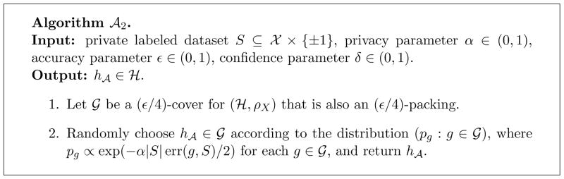
4.1. Algorithm
Our main algorithm
 is given in Figure 1. The first step of the algorithm calculates the distance scale at which it should construct a cover of (
, ρ). This scale is a function of |S|, the size of the input data set S, and can be computed privately because |S| is not sensitive information. A suitable cover of (
, ρ) that is also a suitable packing of (
, ρ) is then constructed; note that such a set always exists because of Lemma 13. In the final step, an exponential mechanism (McSherry and Talwar, 2007) is used to select a hypothesis from the cover with low error. As this step of the algorithm is the only one that uses the input data, the algorithm is α-private as long as this last step guarantees α-privacy.
is given in Figure 1. The first step of the algorithm calculates the distance scale at which it should construct a cover of (
, ρ). This scale is a function of |S|, the size of the input data set S, and can be computed privately because |S| is not sensitive information. A suitable cover of (
, ρ) that is also a suitable packing of (
, ρ) is then constructed; note that such a set always exists because of Lemma 13. In the final step, an exponential mechanism (McSherry and Talwar, 2007) is used to select a hypothesis from the cover with low error. As this step of the algorithm is the only one that uses the input data, the algorithm is α-private as long as this last step guarantees α-privacy.
Figure 1.

Learning algorithm for α-privacy.
4.2. Privacy and learning guarantees
Our first theorem states the privacy guarantee of Algorithm
.
Theorem 7
Algorithm
preserves α-privacy.
Proof
The algorithm only accesses the private dataset S in the final step. Because changing one labeled example in S changes err(g, S) by at most 1, this step is guarantees α-privacy (McSherry and Talwar, 2007).
The next theorem provides an upper bound on the sample requirement of Algorithm
. This bound depends on the doubling dimension d of (
, ρ) and the smoothness parameter κ, as well as the privacy and learning parameters α, ε, δ.
Theorem 8
Let
be a distribution over
× {±1} whose marginal over
is
. There exists a universal constant C > 0 such that for any α, ε, δ ∈ (0, 1), the following holds. If
the doubling dimension d
of (
, ρ) is finite,- is κ-smooth with respect to
,
-
S ⊆ × {±1} is an i.i.d. random sample from
such that
(4) then with probability at least 1 − δ, the hypothesis h ∈
returned by
(S,
, α, ε, δ) satisfies
∈
returned by
(S,
, α, ε, δ) satisfies
The proof of Theorem 8 is stated in Appendix C. If we have prior knowledge that some hypothesis in
has zero error (the realizability assumption), then the sample requirement can be improved with a slightly modified version of Algorithm
. This algorithm, called Algorithm
 , is given in Figure 3 in Appendix C.
Figure 3.
Learning algorithm for α-label privacy.
Theorem 9
Let
be any probability distribution over
×{±1} whose marginal over
is
. There exists a universal constant C > 0 such that for any α, ε, δ ∈ (0, 1), the following holds. If
the doubling dimension d
of (
, ρ) is finite,- is κ-smooth with respect to
,
- S ⊆ × {±1} is an i.i.d. random sample from
such that
(5) - there exists h* ∈ with Pr(x,y) ~
[h*(x) ≠ y] = 0, then with probability at least 1 − δ, the hypothesis h ∈
returned by
(S,
, α, ε, δ) satisfies
Again, the proof of Theorem 9 is in Appendix C.
4.3. Examples
In this section, we give some examples that illustrate the sample requirement of Algorithm
.
First, we consider the example from the lower bound given in the proof of Theorem 5.
Example 1
The domain of the data is
:= [0, 1], and the hypothesis class is
:=
 = {ht: t ∈ [0, 1]} (recall, ht(x) = 1 if and only if x ≥ t). A natural choice for the reference distribution
is the uniform distribution over [0, 1]; the doubling dimension of (
, ρ) is 1 because every interval can be covered by two intervals of half the length. Fix some M > 0 and α ∈ (0, 1), and let η:= 1/(6 + 4 exp(αM)). For z ∈ [η, 1 − η], let
be the distribution on [0, 1] with density
= {ht: t ∈ [0, 1]} (recall, ht(x) = 1 if and only if x ≥ t). A natural choice for the reference distribution
is the uniform distribution over [0, 1]; the doubling dimension of (
, ρ) is 1 because every interval can be covered by two intervals of half the length. Fix some M > 0 and α ∈ (0, 1), and let η:= 1/(6 + 4 exp(αM)). For z ∈ [η, 1 − η], let
be the distribution on [0, 1] with density
Clearly,
is κ-smooth with respect to
for
. Therefore the sample requirement of Algorithm
to learn with α-privacy and excess generalization error ε is at most
which is Õ(M) for constant ε, matching the lower bound from Theorem 5 up to constants.
Next, we consider two examples in which the domain of the unlabeled data
:=
 is the uniform distribution on the unit sphere in ℝn:
and the target hypothesis class
:=
 is the class of linear separators that pass through the origin in ℝn:
The examples will consider two different distributions over
.
A natural reference data distribution in this setting is the uniform distribution over
; this will be our reference distribution
. It is known that d:= sup{ddimr(
, ρ): r ≥ 0} = O(n) (Bshouty et al., 2009).
Example 2
We consider a case where the unlabeled data distribution
is concentrated near an equator of
. More formally, for some vector u ∈
, and γ ∈ (0, 1), we let
be uniform over W:= {x ∈
: |u · x| ≤ γ}; in other words, the unlabeled data lies in a small band of width γ around the equator.
By Lemma 20 (see Appendix C),
is κ-smooth with respect to
for
. Thus the sample requirement of Algorithm
to learn with α-privacy and excess excess generalization error ε is at most
When n is large and , this bound is , where the Õ notation hides factors logarithmic in 1/δ and 1/ε.
Example 3
Now we consider the case where the unlabeled data lies on two diametrically opposite spherical caps. More formally, for some vector u ∈
, and γ ∈ (0, 1), we now let
be uniform over
\W, where W:= {x ∈
: |u · x| ≤ γ}; in other words, the unlabeled data lies outside a band of width γ around the equator.
By Lemma 21 (see Appendix C),
is κ-smooth with respect to
for
. Thus the sample requirement of Algorithm
is to learn with α-privacy and excess generalization error ε is at most:
Thus, for large n and constant γ < 1, the sample requirement of Algorithm
is
. So, even though the smoothness parameter κ is exponential in the dimension n, the sample requirement remains polynomial in n.
5. Lower bounds for learning with α-label privacy
In this section, we provide two lower bounds on the sample complexity of learning with α-label privacy. Our first lower bound holds when α and ε are small (that is, high privacy and high accuracy), and when the hypothesis class has bounded VC dimension V. If these conditions hold, then we show a lower bound of Ω(d/εα) where d is the doubling dimension of the disagreement metric (
, ρ) at some scale.
The main idea behind our bound is to show that differentially private learning algorithms necessarily perform poorly when there is a large set of hypotheses such that every pair in the set labels approximately 1/α examples differently. We then show that such large sets can be constructed when the doubling dimension of the disagreement metric (
, ρ) is high.
5.1. Main results
Theorem 10
There exists a constant c > 0 such that the following holds. Let
be a hypothesis class with VC dimension V < ∞,
be a distribution over
, X be an i.i.d. sample from
of size m, and
be a learning algorithm that guarantees α-label privacy and outputs a hypothesis in
. Let d:= ddim12ε (
, ρ) > 2, and d′:= inf{ddim12r(
, ρ): ε ≤ r < Δ/6} > 2. If
where Δ is the diameter of (
, ρ), then there exists a hypothesis h* ∈
such that with probability at least 1/8 over the random choice of X and internal randomness of
, the hypothesis h returned by
(SX,h*) has classification error
We note that the conditions on α and ε can be relaxed by replacing the VC dimension with other (possibly distribution-dependent) quantities that determine the uniform convergence of ρX to ρ; we used a distribution-free parameter to simplify the argument. Moreover, the condition on ε can be reduced to ε < c for some constant c ∈ (0, 1) provided that there exists a lower bound of Ω(V/ε) to (non-privately) learn
under the distribution
.
The proof of Theorem 10, which is in Appendix D, relies on the following lemma (possibly of independent interest) which gives a lower bound on the empirical error of the hypothesis returned by an α-label private learning algorithm.
Lemma 11
Let X ⊆
be an unlabeled dataset of size m,
be a hypothesis class,
be a learning algorithm that guarantees α-label privacy, and s > 0. Pick any h0 ∈
. If P is an s-packing of BX(h0, 4s) ⊆
, and
then there exists a subset Q ⊆ P such that
|Q| ≥ |P|/2;
for all h ∈ Q, Pr
[
(SX,h) ∉ BX(h, s/2)] ≥ 1/2.
The proof of Lemma 11 is in Appendix D. The next theorem shows a lower bound without restrictions on ε and α. Moreover, this bound also applies when the VC dimension of the hypothesis class is unbounded. However, we note that this bound is weaker in that it does not involve a 1/ε factor, where ε is the accuracy parameter.
Theorem 12
Let
be a hypothesis class,
be a distribution over
, X be an i.i.d. sample from
of size m, and
be a learning algorithm that guarantees α-label privacy and outputs a hypothesis in
. Let d″:= ddim4ε (
, ρ) ≥ 1. If ε ≤ Δ/2 and
where Δ is the diameter of (
, ρ), then there exists h* ∈
such that with probability at least 1/2 over the random choice of X and internal randomness of
, the hypothesis h returned by
(SX,h*) has classification error
In other words, any α-label private algorithm for learning a hypothesis in
with error at most ε ≤ Δ/2 must use at least (d″ − 1) log(2)/α examples. Theorem 12 uses ideas similar to those in (Beimel et al., 2010), but the result is stronger in that it applies to α-label privacy and continuous data domains. A detailed proof is provided in Appendix D.
5.2. Example: linear separators in ℝn
In this section, we show an example that illustrates our label privacy lower bounds. Our example hypothesis class
:=
is the class of linear separators over ℝn that pass through the origin, and the unlabeled data distribution
is the uniform distribution over the unit sphere
. By Lemma 25 (see Appendix D), the doubling dimension of (
, ρ) at any scale r is at least n − 2. Therefore Theorem 10 implies that if α and ε are small enough, any α-label private algorithm
that correctly learns all hypotheses h ∈
with error ≤ ε requires at least
examples. (In fact, the condition on ε can be relaxed to ε ≤ c for some constant c ∈ (0, 1), because Ω(n) examples are needed to even non-privately learn in this setting (Long, 1995).) We also observe that this bound is tight (except for a log(1/δ) factor): as the doubling dimension of
is at most n, in the realizable case, Algorithm
using
:=
learns linear separators with α-label privacy given
examples.
Figure 2.

Learning algorithm for α-privacy under the realizable assumption.
Acknowledgments
KC would like to thank NIH U54 HL108460 for research support. DH was partially supported by AFOSR FA9550-09-1-0425, NSF IIS-1016061, and NSF IIS-713540.
Appendix A. Metric spaces
Lemma 13 (Kolmogorov and Tikhomirov, 1961)
For any metric space (
, ρ) with diameter Δ, and any ε ∈ (0, Δ), there exists an ε-packing of (
, ρ) that is also an ε-cover.
Lemma 14 (Gupta, Krauthgamer, and Lee, 2003)
For any ε > 0 and r > 0, if a metric space (
, ρ) has doubling dimension d and z ∈
, then every ε-packing of (B(z, r), ρ) has cardinality at most (4r/ε)d.
Lemma 15
Let (
, ρ) be a metric space with diameter Δ, and r ∈ (0, 2Δ). If ddimr(
, ρ) ≥ d, then there exists z ∈
such that B(z, r) has an (r/2)-packing of size at least 2d.
Proof
Fix r ∈ (0, 2Δ) and a metric space (
, ρ) with diameter Δ. Suppose that for every z ∈
, every (r/2)-packing of B(z, r) has size less than 2d. For each z ∈
, let Pz be an (r/2)-packing of (B(z, r), ρ) that is also an (r/2)-cover—this is guaranteed to exist by Lemma 13. Therefore, for each z ∈
, B(z, r) ⊆ ∪z′∈Pz
B(z, r/2), and |Pz| < 2d. This implies that ddimr(
, ρ) is less than d.
Appendix B. Uniform convergence
Lemma 16 (Vapnik and Chervonenkis, 1971)
Let
 be a family of measurable functions f:
→ {0, 1} over a space
with distribution
be a family of measurable functions f:
→ {0, 1} over a space
with distribution
 . Denote by
 [f] the empirical average of f over a subset Z ⊆
. Let εm:= (4/m)(log(
[f] the empirical average of f over a subset Z ⊆
. Let εm:= (4/m)(log(
 (2m)) + log(4/δ)), where
(n) is the n-th VC shatter coefficient with respect to
. Let Z be an i.i.d. sample of size m from
. With probability at least 1 − δ, for all f ∈
,
(2m)) + log(4/δ)), where
(n) is the n-th VC shatter coefficient with respect to
. Let Z be an i.i.d. sample of size m from
. With probability at least 1 − δ, for all f ∈
,
Also, with probability at least 1 − δ, for all f ∈
,
Lemma 17
Let
be a hypothesis class with VC dimension V. Fix any δ ∈ (0, 1), and let X be an i.i.d. sample of size m ≥ V/2 from
. Let εm:= (8V log(2em/V) + 4 log(4/δ))/m. With probability at least 1 − δ, for all pairs of hypotheses {h, h′} ⊆
,
Also, with probability at least 1 − δ, for all pairs of hypotheses {h, h′} ⊆
,
Proof
This is an immediate consequence of Lemma 16 as applied to the function class
:= {x ↦
[h(x) ≠ h′ (x)]: h, h′ ∈
}, which has VC shatter coefficients
(2m) ≤
 (2m)2
≤ (2em/V)2V by Sauer’s Lemma.
(2m)2
≤ (2em/V)2V by Sauer’s Lemma.
Appendix C. Proofs from Section 4
C.1. Some lemmas
We first give two simple lemmas. The first one, Lemma 18 states some basic properties of the exponential mechanism.
Lemma 18 (McSherry and Talwar, 2007)
Let I be a finite set of indices, and let ai ∈ ℝ for all i ∈ I. Define the probability distribution p:= (pi: i ∈ I) where pi ∝ exp(−ai) for all i ∈ I. If j ∈ I is drawn at random according to p, then the following holds for any element i0 ∈ I and any t ∈ ℝ.
Let i ∈ I. If ai ≥ t, then Prj−p[j = i] ≤ exp(−(t − ai0)).
Prj~p[aj ≥ ai0+ t] ≤ |I| exp(−t).
Proof
Fix any i0 ∈ I and t ∈ ℝ. To show the first part of the lemma, note that for any i ∈ I with ai ≥ t, we have
For the second part, we apply the inequality from the first part to all i ∈ I such that ai ≥ ai0 + t, so
The next lemma is consequences of smoothness between distributions
and
.
Lemma 19
If
is κ-smooth with respect to
, then for all ε > 0, every ε-cover of (
, ρ) is a κε-cover of (
, ρ).
Proof
Suppose C is an ε-cover of (
, ρ). Then, for any h ∈
, there exists h′ ∈ C such that ρ(h, h′) ≤ ε. Fix such a pair h, h′, and let A := {x ∈ χ : h(x) ≠ h′(x)} be the subset of χ on which h and h′ disagree. As
is κ-smooth with respect to
, by definition of smoothness,
and thus C is a κε-cover of (
, ρ).
C.2. Proof of Theorem 8
First, because of the lower bound on m := |S| from (4), the computed value of κ̂ in the first step of the algorithm must satisfy κ̂ ≥ κ. Therefore,
is also κ̂-smooth with respect to
. Combining this with Lemma 19,
is an (ε/4)-cover of (
, ρ). Moreover, as
is also an (ε/4κ̂)-packing of
, from Lemma 14, the cardinality of
is at most |
| ≤ (16κ̂/ε)d .
.
Define err(h) := Pr(x,y)~
[h(x) ≠ y]. Suppose that h* ∈
minimizes err(h) over h ∈
. Let g0 ∈
be an element of
such that ρ(h*, g0) ≤ ε/4; g0 exists as
is an (ε/4)-cover of (
, ρD). By the triangle inequality, we have that:
| (6) |
Let E be the event that maxg∈
 | err(g) − err(g, S)| > ε/4, and Ē be its complement. By Hoeffding’s inequality, a union bound, and the lower bound on |S|, we have that for a large enough value of the constant C in Equation (4),
In the event Ē, we have err(h) ≥ err(h, S) − ε/4 and err(g0) ≤ err(g0, S) + ε/4 because both h and g0 are in
. Therefore,
Here, the first step follows from (7), and the final three inequalities follow from Lemma 18 (using ag = α|S| err(g, S)/2 for g ∈
), the upper bound on |
|, and the lower bound on m in (4).
C.3. Proof of Theorem 9
The proof is very similar to the proof of Theorem 8.
First, because of the lower bound on m := |S| from (5), the computed value of κ̂ in the first step of the algorithm must satisfy κ̂ ≥ κ. Therefore,
is also κ̂-smooth with respect to
. Combining this with Lemma 19, as
is an (ε/4κ̂)-cover of
,
is an (ε/4)-cover of (
, ρ). Moreover, as
is also an (ε/4κ̂)-packing of
, from Lemma 14, the cardinality of
is at most |
| ≤ (16κ̂/ε)d.
Define err(h) := Pr(x,y)~
[h(x) ≠ y]. Suppose that h* ∈
minimizes err(h) over h ∈
. Recall that from the realizability assumption, err(h*) = 0. Let g0 ∈
be an element of
such that ρdcl12;(h*, g0) ≤ ε/4; g0 exists as
is an (ε/4)-cover of (
, ρ). By the triangle inequality, we have that:
| (7) |
We define two events E1 and E2. Let
 ⊂ G be the set of all g ∈
for which err(g) ≥ ε. The event E1 is the event that ming∈
⊂ G be the set of all g ∈
for which err(g) ≥ ε. The event E1 is the event that ming∈
 err(g, S) > 9ε/10, and let Ē1 be its complement. Applying the multiplicative Chernoff bounds, for a specific g ∈
,
err(g, S) > 9ε/10, and let Ē1 be its complement. Applying the multiplicative Chernoff bounds, for a specific g ∈
,
The quantity on the right hand side is at most
for a large enough constant C in Equation (5). Applying an union bound over all g ∈
, we get that
| (8) |
We define E2 as the event that err(g0, S) ≤ 3ε/4, and Ē2 as its complement. From a standard multiplicative Chernoff bound, with probability at least 1 − δ/4,
Thus, if |S| ≥ (3/ε) log(4/δ), which is the case due to Equation (5),
| (9) |
Therefore, we have
Here, the second step follows from the definition of events E1 and E2 and from Equations (8) and (9), the third step follows from simple algebra, the fourth step follows from Lemma 18, the fifth step from the bound on |
| and the final step from Equation (5).
C.4. Examples
Lemma 20
Let
be uniform over the unit sphere
, and let
be defined as in Example 2. Then,
is
with respect to
.
Proof
From (Ball, 1997), we know that Prx~
[x ∈ W] ≥ 1 − 2 exp(−nγ2/2). Thus, for any set A ⊆
, we have
This means
is κ-smooth with respect to
for 1
Lemma 21
Let
uniform over the unit sphere
and let
be defined as in Example 3. Then,
is
with respect to
.
Proof
From (Ball, 1997), we know that Prx~
[x ∈
\ W] = Prx~
[x ∉ W] ≥ ((1 − γ)/2)(n−1)/2. Therefore, for any A ⊆
, we have
This means
is κ-smooth with respect to
for
Appendix D. Proofs from Section 5
D.1. Some lemmas
Lemma 22
Let S := {(x1, y1), …, (xm, ym)} ⊆ χ × {±1} be a labeled dataset of size m, α ∈ (0, 1), and k ≥ 0.
- If a learning algorithm guarantees α-privacy and outputs a hypothesis from
, then for all
with
for at least |S| − k such examples,
-
If a learning algorithm
guarantees α-label privacy and outputs a hypothesis from
, then for all
with
for at least |S| − k such labels,
Proof
We prove just the first part, as the second part is similar. For a labeled dataset S′ that differs from S in at most k pairs, there exists a sequence of datasets S(0), …, S(ℓ) with ℓ ≤ k such that S(0) = S′, S(ℓ) = S, and S(j) differs from S(j+1) in exactly one example for 1 ≤ j < ℓ. In this case, if
guarantees α-privacy, then for all
⊆
,
and therefore
Lemma 23
There exists a constant C > 1 such that the following holds. Let
be a hypothesis class with VC dimension V, and let
be distribution over χ. Fix any r ∈ (0, 1), and let X be an i.i.d. sample of size m from
. If
then the following holds with probability at least 1/2:
every pair of hypotheses{h, h′} ⊆
for which ρX(h, h′) > 2r has ρ(h, h′) > r;for all h0 ∈
, every (6r)-packing of (B(h0, 12r), ρ) is a (4r)-packing of (BX(h0, 16r), ρX).
Proof
This is a consequence of Lemma 17. To show the first part, we plug in Lemma 17 with εm = r/2.
To show the second part, we use two applications of Lemma 17. Let h and h′ be any two hypotheses in any (6r)-packing of (B(h0, 12r), ρ); we first use Lemma 17 with εm = r/3 to show that for all such h and h′, ρX(h, h′) > 4r. Next we need to show that all h in any (6r)-packing of (B(h0, 12r), ρ) has ρX(h, h0) ≤ 16r; we show this through a second application of Lemma 17 with εm = r/3.
D.2. Proof of Theorem 12
We prove the contrapositive: that if ε ≤ Δ/2 and PrX~
 ,
[
(SX,h*) ∈ B(h*, ε)] > 1/2 for all h* ∈ H, then m > log(2d″−1)/α. So pick any ε ≤ Δ/2. By Lemma 15, there exists an h0 ∈
and P ⊆
such that P is a (2ε)-packing of (B(h0, 4ε), ρ) of size ≥ 2d″. For any h, h′ ∈ P such that h ≠ h′, we have B(h, ε) ∩ B(h′, ε) = ∅ by the triangle inequality. Therefore for any h ∈ P and any X′ ⊆ χ of size m,
,
[
(SX,h*) ∈ B(h*, ε)] > 1/2 for all h* ∈ H, then m > log(2d″−1)/α. So pick any ε ≤ Δ/2. By Lemma 15, there exists an h0 ∈
and P ⊆
such that P is a (2ε)-packing of (B(h0, 4ε), ρ) of size ≥ 2d″. For any h, h′ ∈ P such that h ≠ h′, we have B(h, ε) ∩ B(h′, ε) = ∅ by the triangle inequality. Therefore for any h ∈ P and any X′ ⊆ χ of size m,
where the second inequality follows by Lemma 22 because SX′,h and SX′,h′ can differ in at most (all) m labels. Now integrating both sides with respect to X′ ~
 shows that if PrX~
,
[
(SX,h*) ∈ B(h*, ε)] > 1/2 for all h* ∈
, then for any h ∈ P,
shows that if PrX~
,
[
(SX,h*) ∈ B(h*, ε)] > 1/2 for all h* ∈
, then for any h ∈ P,
which in turn implies m > log(|P| − 1)/α ≥ log(2d″ − 1)/α ≥ log(2d″−1)/α, as d″ is always ≥ 1.
D.3. Proof of Lemma 11
Let h0 ∈
and P be an s-packing of BX(h0, 4s) ⊆
. Say the algorithm
is good for h if Pr[
(SX,h) ∈ BX(h, s/2)] ≥ 1/2. Note that
is not good for h ∈ P if and only if Pr[
(SX,h) ∉/BX(h, s/2)] > 1/2. Therefore, it suffices to show that if
is good for at least |P|/2 hypotheses in P, then m ≥ (log((|P|/2) −1)/(8αs).
By the triangle inequality and the fact that P is an s-packing, BX(h, s/2)∩BX(h′, s/2) = ∅ for all h, h′ ∈ P such that h ≠ h′. Therefore for any h ∈ P,
Moreover, for all h, h′ ∈ P, we have ρX(h, h′) ≤ ρX(h0, h) + ρX(h0, h′) ≤ 8s by the triangle inequality, so SX,h and SX,h′ differ in at most 8sm labels. Therefore Lemma 22 implies
for all h, h′ ∈ P. If
is good for at least |P|/2 hypotheses h′ ∈ P, then for any h ∈ P such that
is good for h, we have
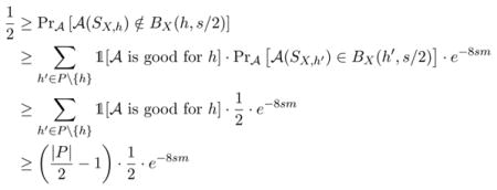 |
which in turn implies m ≥ log((|P|/2) − 1)/(8s).
D.4. Proof of Theorem 10
We need the following lemma.
Lemma 24
There exists a constant C > 1 such that the following holds. Let
be a hypothesis class with VC dimension V,
be a distribution over χ, X be an i.i.d. sample from
of size m,
be a learning algorithm that guarantees α-label privacy and outputs a hypothesis in
, and Δ be the diameter of (
, ρ). If r ∈ (0, Δ/6) and
where d := ddim12r(
, ρ), then there exists a hypothesis h* ∈
such that
Proof
First, assume r and m satisfy the conditions in the lemma statement, where C is the constant from Lemma 23. Also, let h0 ∈
and P ⊆
be such that P is a (6r)-packing of (B(h0, 12r), ρ) of size |P| ≥ 2d; the existence of such an h0 and P is guaranteed by Lemma 15.
We first define some events in the sample space of X and
. For each h ∈
, and a sample X, let E1(h, X) be the event that
Given a sample X, let φ(X) be a 0/1 random variable which is 1 when the following conditions hold:
every pair of hypotheses{h, h′} ⊆
for which ρX(h, h′) > 2r has ρ(h, h′) > r; andfor all h0 ∈
, every (6r)-packing of (B(h0, 12r), ρ) is a (4r)-packing of (BX(h0, 16r), ρX)
(i.e., the conclusion of Lemma 23). Note that conditioned on E1(h, X) and φ(X) = 1, we have ρX(h,
(SX,h)) > 2r and thus ρ(h,
(SX,h)) > r, so PrX~
,
[E1(h, X), (φ(X) = 1)] ≤ PrX~
,
[ρ(h,
(SX,h)) > r]. Therefore it suffices to show that there exists h* ∈
such that PrX~
,
[E1(h*, X), (φ(X) = 1)] ≥ 1/8.
The lower bound on m and Lemma 23 ensure that 1
| (10) |
Also, if the unlabeled sample X is such that φ(X) = 1 holds, then the set P is a (4r)-packing of (BX(h0, 16r), ρX). Therefore, the upper bound on m and Lemma 11 (with s = 4r) imply that for all such X, there exists Q ⊆ P of size at least |P|/2 such that Pr[E1(h, X) | φ(X) = 1] ≥ 1/2 for all h ∈ Q. In other words,
| (11) |
Combining Equations (10) and (11) gives
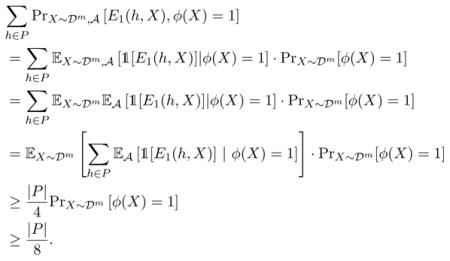 |
Here the first step follows because φ(X) is a 0/1 random variable, the fourth step follows from Equation (11) and the fifth step follows from Equation (10).
Therefore there exists some h* ∈ P such that PrX~
,
[E1(h*, X), φ(X) = 1] ≥ 1/8.
Proof [Proof of Theorem 10]
Assume
where C is the constant from Lemma 24. The proof is by case analysis, based on the value of m.
Case 1: m < 1/(4ε)
Since ε < Δ/2, Lemma 15 implies that there exists a pair{h, h′} ⊆
such that ρ(h, h′) > 2ε but ρ(h, h′) ≤ 4ε. Using the bound on m and the fact ε ≤ 1/5, we have
This means that PrX~
[h:=
(SX,h) =
(SX,h′)] ≥ 1/8. By the triangle inequality, B(h, ε) ∩ B(h′, ε) = ∅. So if, say, PrX~
,
[h ∈ B(h, ε)] ≥ 1/8, then PrX~
,
[h ∉/B(h′, ε)] ≥1/8. Therefore PrX~
,
[h ∉/B(h*, ε)] ≥ 1/8 for at least one h* ∈ {h, h′}.
Case 2: 1/(4ε) ≤ m < (CV/ε) log(C/ε)
First, let r > 0 be the solution to the equation (CV/r) log(C/r) = m, so r > ε. Moreover, the bound on m and ε imply
so r < Δ/6. Finally, using the bound on α, definition of d′, and fact r > ε, we have
where d″ := ddim12r(
, ρ); this implies
The conditions of Lemma 24 are thus satisfied, which means there exists h* ∈
such that PrX~
,
[
(SX,h*) ∉/B(h*, r)] ≥ 1/8.
Case 3: (CV/ε) log(C/ε) ≤ m < log(2d−1 − 1)/(32αε)
The conditions of Lemma 24 are satisfied in this case with r := ε < Δ/6, so there exists h* ∈ H such that PrX~
,
[ρD(h*,
(SX,h*)) > ε] ≥ 1/8.
D.5. Example
The following lemma shows that if
is the uniform distribution on
, then ddimr(
, ρ) ≥ n − 2 for all scales r > 0.
Lemma 25
Let
:=
be the class of linear separators through the origin in ℝn and
be the uniform distribution on
. For any u ∈
and any r > 0, there exists an (r/2)-packing of (B(hu, r), ρ) of size at least 2n−2.
Proof
Let μ be the uniform distribution over
; notice that this is also the uniform distribution over
.
We call a pair hypotheses hv and hw in
close if ρ (hv, hw) ≤ r/2. Observe that if any set of hypotheses has no close pairs, then it is an (r/2)-packing.
Using a technique due to Long (1995), we now construct an (r/2)-packing of B(hu, r) by first randomly choosing hypotheses in B(hu, r), and then removing hypotheses until no close pairs remain. First, we bound the probability p that two hypotheses hv and hw, chosen independently and uniformly at random from B(hu, r), are close:
where the second-to-last equality follows by symmetry, and the last equality follows by the fact that B(hu, r) corresponds to a (n−1)-dimensional spherical cap of
. Now, choose N := 2n−1 hypotheses hv1, …, hvN independently and uniformly at random from B(hu, r). The expected number of close pairs among these N hypotheses is
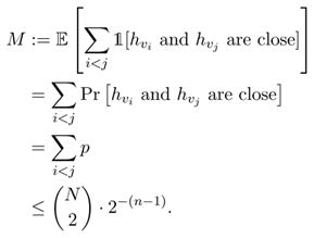 |
Therefore, there exists N hypotheses hv1, …, hvN in B(hu, r) among which there are at most M close pairs. Removing one hypothesis from each such close pair leaves a set of at least N − M hypotheses with no close pairs—this is our (r/2)-packing of B(hu, r). Since N = 2n−1, the cardinality of this packing is at least
Appendix E. Upper bounds for learning with α-label privacy
Algorithm
 for learning with α-label privacy, given in Figure 3, differs from the algorithms for learning with α-privacy in that it is able to use the unlabeled data itself to construct a finite set of candidate hypotheses. The algorithm and its analysis are very similar to work due to Chaudhuri et al. (2006); we give the details for completeness.
Theorem 26
Algorithm
preserves α-label privacy.
Proof
The algorithm only accesses the labels in S in the final step. It follows from standard arguments in (McSherry and Talwar, 2007) that α-label privacy is guaranteed.
Theorem 27
Let
be any probability distribution over χ × {±1} whose marginal over χ is
. There exists a universal constant C > 0 such that for any α, ε, δ ∈ (0, 1), the following holds. If S ⊆ χ × {±1} is an i.i.d. random sample from
of size
where η := infh′∈
 Pr(x,y)~
[h′(x) ≠ y] and V is the VC dimension of
; then with probability at least 1 − δ, the hypothesis h ∈
returned by
(S, α, ε, δ) satisfies
Pr(x,y)~
[h′(x) ≠ y] and V is the VC dimension of
; then with probability at least 1 − δ, the hypothesis h ∈
returned by
(S, α, ε, δ) satisfies
Remark 28
The first term in the sample size requirement (which depends on VC dimension) can be replaced by distribution-based quantities used for characterizing uniform convergence such as those based on l1-covering numbers (Pollard, 1984).
Proof
Let err(h) := Pr(x,y)~
[h(x) ≠ y], and let h* ∈
minimize err(h) over h ∈
. Let S := {(x1, y1), …, (xm, ym)} be the i.i.d. sample drawn from
, and X := {x1, …, xm} be the unlabeled components of S. Let g0 ∈
minimize err(g, S) over g ∈
. Since
is an (ε/4)-cover for (
, ρX), we have that err(g0, S) ≤ infh′∈
err(h′, S) + ε/4. Since
is also an (ε/4)-packing for (
, ρX), we have that |
| ≤
 (
, ρX) (Pollard, 1984). Let
:= {fh : h ∈ H} where fh(x, y) :=
[h(x) ≠ y]. We have
(
, ρX) (Pollard, 1984). Let
:= {fh : h ∈ H} where fh(x, y) :=
[h(x) ≠ y]. We have
 [fh(x, y)] = err(h) and m−1 Σ(x,y)∈S fh(x, y) = err(h, S). Let E be the event that for all h ∈ H,
where εm := (8V log(2em/V) + 4 log(16/δ))/m. By Lemma 16, the fact
 (
, n) = S(H, n), and union bounds, we have PrS~
(
, n) = S(H, n), and union bounds, we have PrS~
 [E] ≥ 1 − δ/2. Now let E′ be the event that
where tm := 2 log(2
 [|
|]/δ)/(αm). The probability of E′ can be bounded as
[|
|]/δ)/(αm). The probability of E′ can be bounded as
where the first inequality follows from Lemma 18, and the second inequality follows from the definition of tm. By the union bound, PrS~
,
[E ∩ E′] ≥ 1 −δ. In the event E ∩ E′, we have
since err(g0, S) ≤ infh′∈
err(h′, S) + ε/4 ≤ err(h*, S) + ε/4. By various algebraic manipulations, this in turn implies
for some constant C′ > 0. The lower bound on m now implies the theorem.
Footnotes
Here the Õ notation hides factors logarithmic in 1/ε
Contributor Information
Kamalika Chaudhuri, Email: kamalika@cs.ucsd.edu, University of California, San Diego, 9500 Gilman Drive #0404, La Jolla, CA 92093-0404.
Daniel Hsu, Email: dahsu@microsoft.com, Microsoft Research New England, One Memorial Drive, Cambridge, MA 02142.
References
- Agrawal R, Srikant R. Privacy-preserving data mining. SIGMOD Rec. 2000;29(2):439–450. doi: http://doi.acm.org/10.1145/335191.335438. [Google Scholar]
- Backstrom Lars, Dwork Cynthia, Kleinberg Jon M. Wherefore art thou r3579x?: anonymized social networks, hidden patterns, and structural steganography. In: Williamson Carey L, Zurko Mary Ellen, Patel-Schneider Peter F, Shenoy Prashant J., editors. WWW. ACM; 2007. pp. 181–190. [Google Scholar]
- Ball K. An elementary introduction to modern convex geometry. In: Levy Silvio., editor. Flavors of Geometry. Vol. 31. 1997. [Google Scholar]
- Barak B, Chaudhuri K, Dwork C, Kale S, McSherry F, Talwar K. Privacy, accuracy, and consistency too: a holistic solution to contingency table release. PODS. 2007:273–282. [Google Scholar]
- Beimel Amos, Kasiviswanathan Shiva Prasad, Nissim Kobbi. Bounds on the sample complexity for private learning and private data release. TCC. 2010:437–454. [Google Scholar]
- Blum A, Dwork C, McSherry F, Nissim K. Practical privacy: the sulq framework. PODS. 2005:128–138. [Google Scholar]
- Blum A, Ligett K, Roth A. A learning theory approach to non-interactive database privacy. In: Ladner RE, Dwork C, editors. STOC. ACM; 2008. pp. 609–618. [Google Scholar]
- Bshouty Nader H, Li Yi, Long Philip M. Using the doubling dimension to analyze the generalization of learning algorithms. J Comput Syst Sci. 2009;75(6):323–335. [Google Scholar]
- Chaudhuri K, Dwork C, Kale S, McSherry F, Talwar K. Manuscript. 2006. Learning concept classes with privacy. [Google Scholar]
- Chaudhuri K, Monteleoni C, Sarwate A. Differentially private empirical risk minimization. Journal of Machine Learning Research. 2011 [PMC free article] [PubMed] [Google Scholar]
- Chaudhuri Kamalika, Mishra Nina. When random sampling preserves privacy. In: Dwork Cynthia., editor. CRYPTO. Vol. 4117. Springer; 2006. pp. 198–213. Lecture Notes in Computer Science. [Google Scholar]
- Dasgupta Sanjoy. Coarse sample complexity bounds for active learning. NIPS. 2005 [Google Scholar]
- Dwork C, McSherry F, Nissim K, Smith A. Calibrating noise to sensitivity in private data analysis. 3rd IACR Theory of Cryptography Conference; 2006. pp. 265–284. [Google Scholar]
- Evfimievski A, Gehrke J, Srikant R. Limiting privacy breaches in privacy preserving data mining. PODS. 2003:211–222. [Google Scholar]
- Yoav Freund H, Seung Sebastian, Shamir Eli, Tishby Naftali. Selective sampling using the query by committee algorithm. Machine Learning. 1997;28(2–3):133–168. [Google Scholar]
- Ganta Srivatsava Ranjit, Kasiviswanathan Shiva Prasad, Smith Adam. Composition attacks and auxiliary information in data privacy. KDD. 2008a:265–273. [Google Scholar]
- Ganta Srivatsava Ranjit, Kasiviswanathan Shiva Prasad, Smith Adam. Composition attacks and auxiliary information in data privacy. KDD. 2008b:265–273. [Google Scholar]
- Gupta Anupam, Krauthgamer Robert, Lee James R. Bounded geometries, fractals, and low-distortion embeddings. FOCS. 2003:534–543. [Google Scholar]
- Gupta Anupam, Hardt Moritz, Roth Aaron, Ullman Jonathan. Privately releasing conjunctions and the statistical query barrier. STOC. 2011 [Google Scholar]
- Hardt Moritz, Talwar Kunal. On the geometry of differential privacy. STOC. 2010:705–714. [Google Scholar]
- Jones Rosie, Kumar Ravi, Pang Bo, Tomkins Andrew. “i know what you did last summer”: query logs and user privacy. CIKM ‘07: Proceedings of the sixteenth ACM conference on Conference on information and knowledge management; New York, NY, USA. ACM; 2007. pp. 909–914. doi: http://doi.acm.org/10.1145/1321440.1321573. [Google Scholar]
- Kasiviswanathan SA, Lee HK, Nissim K, Raskhodnikova S, Smith A. What can we learn privately? Proc of Foundations of Computer Science. 2008 [Google Scholar]
- Kasiviswanathan Shiva Prasad, Smith Adam. A note on differential privacy: Defining resistance to arbitrary side information. CoRR. 2008 abs/0803.3946. [Google Scholar]
- Kolmogorov A, Tikhomirov V. ε-entropy and ε-capacity of sets in function spaces. Translations of the American Mathematical Society. 1961;17:277–364. [Google Scholar]
- Long PM. On the sample complexity of pac learning halfspaces against the uniform distribution. IEEE Transactions on Neural Networks. 1995;6(6):1556–1559. doi: 10.1109/72.471352. [DOI] [PubMed] [Google Scholar]
- Machanavajjhala A, Gehrke J, Kifer D, Venkitasubramaniam M. l-diversity: Privacy beyond k-anonymity. Proc of ICDE. 2006 [Google Scholar]
- McAllester David A. Some pac-bayesian theorems. COLT. 1998:230–234. [Google Scholar]
- McSherry Frank, Mironov Ilya. Differentially private recommender systems: building privacy into the net. KDD ‘09: Proceedings of the 15th ACM SIGKDD international conference on Knowledge discovery and data mining; New York, NY, USA. ACM; 2009. pp. 627–636. doi: http://doi.acm.org/10.1145/1557019.1557090. [Google Scholar]
- McSherry Frank, Talwar Kunal. Mechanism design via differential privacy. FOCS. 2007:94–103. [Google Scholar]
- Narayanan Arvind, Shmatikov Vitaly. Robust de-anonymization of large sparse datasets. IEEE Symposium on Security and Privacy; Oakland, CA, USA. May 2008; IEEE Computer Society; pp. 111–125. [Google Scholar]
- Nissim Kobbi, Raskhodnikova Sofya, Smith Adam. Smooth sensitivity and sampling in private data analysis. In: Johnson David S, Feige Uriel., editors. STOC. ACM; 2007. pp. 75–84. [Google Scholar]
- Pollard D. Convergence of Stochastic Processes. Springer-Verlag; 1984. [Google Scholar]
- Roth Aaron. Differential privacy and the fat-shattering dimension of linear queries. APPROX-RANDOM. 2010:683–695. [Google Scholar]
- Sweeney L. k-anonymity: a model for protecting privacy. Int J on Uncertainty, Fuzziness and Knowledge-Based Systems. 2002 [Google Scholar]
- Vapnik VN, Chervonenkis AY. On the uniform convergence of relative frequencies of events to their probabilities. Theory of Probability and Its Applications. 1971;16(2):264–280. [Google Scholar]
- Wang Rui, Li Yong Fuga, Wang XiaoFeng, Tang Haixu, Zhou Xiao yong. Learning your identity and disease from research papers: information leaks in genome wide association study. ACM Conference on Computer and Communications Security; 2009. pp. 534–544. [Google Scholar]
- Yao Andrew Chi-Chih. Protocols for secure computations (extended abstract) FOCS. 1982:160–164. [Google Scholar]
- Zhou Shuheng, Ligett Katrina, Wasserman Larry. Differential privacy with compression. Proc of ISIT. 2009 [Google Scholar]