One third of dynamic protein expression profiles can be predicted by simple rate equations

Abstract

Cells respond to environmental stimuli with expression changes at both the mRNA and protein level, and a plethora of known and unknown regulators affect synthesis and degradation rates of the resulting proteins. To investigate the major principles of gene expression regulation in dynamic systems, we estimated protein synthesis and degradation rates from parallel time series data of mRNA and protein expression and tested the degree to which expression changes can be modeled by a set of simple linear differential equations. Examining three published datasets for yeast responding to diamide, rapamycin, and sodium chloride treatment, we find that almost one-third of genes can be well-modeled, and the estimated rates assume realistic values. Prediction quality is linked to low measurement noise and the shape of the expression profile. Synthesis and degradation rates do not correlate within one treatment, consistent with their independent regulation. When performing robustness analyses of the rate estimates, we observed that most genes adhere to one of two major modes of regulation, which we term synthesis- and degradation-independent regulation. These two modes, in which only one of the rates has to be tightly set, while the other one can assume various values, offer an efficient way for the cell to respond to stimuli and re-establish proteostasis. We experimentally validate degradation-independent regulation under oxidative stress for the heatshock protein Ssa4.

Introduction

Control of gene expression is a complex process involving tight regulation of rates of mRNA and protein synthesis and degradation by a variety of factors. Under environmental stress, cells adjust these rates to adequately respond at multiple levels of gene expression regulation. For example, during the environmental stress response in yeast, stress-response genes are transcriptionally up-regulated, while global protein synthesis and growth related genes are down-regulated^{1, 2}. During mild oxidative stress, proteosomal protein degradation increases, but decreases at higher oxidant levels³. Ribosomal runoff and transit times are generally slower upon H₂O₂ exposure, but the mRNAs of stress-related proteins are increasingly associated with ribosomes, suggesting enhanced translation^{4, 5}. Exposure to hydrogen peroxide causes a rapid, but temporary inhibition of protein synthesis at the level of translation⁴. Adaptation to stress, in turn, lasts for many hours in mammalian cells⁶. In general, the relationship between translation changes under stress affecting genes and their 5’UTRs, e.g. upstream Open Reading Frames, is a very complex and highly dynamic process⁷.

The relative contributions of the rates of synthesis and degradation to setting final protein concentrations have been a matter of debate and have been explored using both steady state (cross-sectional) and dynamic (time-series, longitudinal) experimental designs. A study in a differentiating human THP-1 myelomonocytic leukemia cell line found that synthesis rates are predominantly responsible for large changes in protein expression, while degradation rates tend to stay constant⁸. In contrast, another study of mammalian cells under TNAα stimulation proposes that degradation rates play a key role in controlling systematic proteome changes during perturbations⁹. Recent evidence has demonstrated that synthesis and degradation of RNA and proteins may be coupled in yeast¹⁰ and in mammalian cell^{8, 9}. Such coupling can complicate the gene expression patterns observed in response to a stimulus.

The enormous complexity of the response has motivated the search for regulatory factors that, at the level of transcription, translation, and degradation, impact the shape of expression profiles. However, in this study we reverse this problem and ask which types of time-dependent expression profiles could the cell achieve without employing regulatory factors, but by assuming simple linear relationships between the contributing synthesis and degradation rates. In other words, for which profile shapes are additional regulatory factors not immediately necessary? Our question is motivated by the fact that even simple systems of coupled differential equations can often account for very complex behaviors: for example, in physics, it is known that three ordinary differential equations known as Lorenz equations can exhibit complex chaotic behaviors¹¹. Here, we used a system of linear differential equations to model time-dependent protein expression changes in yeast cells responding to environmental stress, and successfully do so for a third of the genes. Using robustness analysis, we also explored the relative contributions of synthesis and degradation regulation to setting final protein concentrations. We find evidence that most well-predicted proteins generally regulate either synthesis or degradation, but not both.

Materials and methods

Data sets used and data preprocessing

We used three published time course datasets where both protein and RNA levels were measured in yeast responding to a stimulus (Table 1). The types of stimuli include diamide^{1, 12, 13}, rapamycin¹⁴, and sodium chloride induced osmotic stress¹⁵. These time series are each composed of between six to eight time points collected over up to 360 min. The Diamide dataset contains estimates of absolute mRNA and protein concentrations, reported as molecules/cell. The other two datasets report relative concentrations, i.e. normalized to the value at time 0. The fourth, steady-state dataset comprises published western blot measurements of decreases in protein concentrations to derive protein half-lives (and therefore degradation rates)¹⁶, and translation rate estimates based on polysome profiling measurements and assumptions on general speeds of translation¹⁷. To ensure high-quality predictions, we only used the data for genes with one or no missing data points, leaving 530, 683, and 328 genes to examine in the Diamide, Sodium chloride, and Rapamycin data set, respectively.

Table 1. Datasets and main relationships.

Summary of experimental methods referenced in this paper and the key results. a.u. – arbitrary units, P – protein concentration, R – RNA concentration

Data set	Diamide	Rapamycin	Sodium Chloride	Unstressed
Reference	Vogel 201113; Gasch 20001	Fournier 201014	Lee 201115	Fraser 200417; Belle 200616
mRNA data	Dual-channel microarray	Dual-channel microarray	Dual-channel microarray	Translation: computational analysis of polysome profile data
Protein quantification method	LC-MS/MS	LC-MS/MS	LC-MS/MS	Western-blot of cycloheximide treated cells
Treatment	Diamide	Rapamycin	High osmolarity	none
Measurement time (min)	120	360	240	none
Number of genes used for modeling	530	328	683	3343
Number of well-predicted genes (FDR<30%)	116	94	233	n/a
Pearson correlation between log(ks) and log(kd)	0.45	0.80	0.76	−0.25
Median of ks	4.0 P/(R*min)	0.010 a.u.	0.27 a.u.	5.8 P/(R*min)
Median half-lives (min)	41	109	204	45

Mathematical model to estimate protein synthesis and degradation rates

The goal of this analysis is the estimation of protein expression changes in response to a stimulus. We use first-order equations to estimate protein synthesis and degradation rates from time series data of protein and matching mRNA concentration changes. Each protein's time-dependent concentration can be modeled by the simple ordinary differential equation (ODE):

$$\frac{dP}{dt}=k_{s}R(t)-k_{d}P(t)$$ [Eq. 1]

where P(t) is the concentration of the protein at time t R(t) is the amount of RNA that codes for the protein present in the cell at time t; k_s is the rate of protein synthesis, and k_d is the rate of protein degradation. This ODE is a commonly used first approximation of the processes governing the central dogma of biology^{8, 9, 13, 15}. In this model, k_s and k_d are assumed constant over the entire measurement time. $\frac{dP}{dt}$ represents the change of protein abundance at time t Since measurements are done at discrete time points, the ODE can be approximated by a finite-difference approximation and rewritten as:

$$P(t_{n+1})=P(t_n)+(k_{s}R(t_n)+k_{d}P(t_n))\Delta t$$ [Eq. 2]

where t_n and t_n+1 represent the times of two consecutive measurements, Δt = t_n+1−t_n. While the concentrations R(t_n) and P(t_n) are experimentally measured for each time point t_n the constants k_s and k_d will be inferred in a way that fits the data point optimally given the finite-difference approximation -- a relatively safe assumption for these datasets, composed of primarily small time intervals relative to estimated and previously published rates. The optimization includes two biophysical constraints k_s ≥ 0 and k_s ≥ µ where µ is the rate of protein degradation due solely to cell division, assuming an equal distribution of protein molecules between the two daughter cells. The division time µ was measured experimentally for each of the three datasets or taken from the publication.

The finite-difference approximation, which assumes linear behavior between consecutive time points, is expected to hold because most of the measurements in all three datasets are concentrated at the beginning of the time series, where most proteins experience the most rapid changes in expression. This setup allows the time differences Δt to be small enough for most protein abundances not to exhibit a complex behavior between consecutive time points.

To perform linear regression, the ODE is further rearranged into:

$$y(t_n)=K_{s}R(t_n)-k_{d_o}P(t_n)$$ [Eq. 3]

where k_do = k_d – µ and y(t_n) is defined as

$$y(t_n)\underset{¯}{\underset{¯}{def}}\frac{P(t_{n+1})-P(t_n)}{\Delta t}+\mu P(t_n)$$ [Eq. 4]

In matrix form, Eq. 3 is then

$$\left[\begin{array}{cc}R(t_1)\hfill & P(t_1)\hfill \\ ⋮\hfill & ⋮\hfill \\ R(t_n)\hfill & P(t_n)\hfill \end{array}\right]\left[\begin{array}{c}{k}_s\hfill \\ k_d\hfill \end{array}\right]=\left[\begin{array}{c}y(t_1)\hfill \\ ⋮\hfill \\ y(t_n)\hfill \end{array}\right]$$ [Eq. 5]

We built a matrix according to Eq. 5 for each gene separately and performed non-negative least squares regression using the nnls R package(http://cran.r-project.org/web/packages/nnls/index.html). Regression yields non-negative values for k_do and k_s, thus providing us with the estimates of the synthesis rate k_s and the degradation rate k_d. The quality of the model fit is evaluated separately for each gene.

Prediction Quality Measures (Error Models)

To assess the quality of the regression, we used the parameters k_s and k_d to predict protein expression profiles according to the ODE model and compare them to the observed profiles. The predicted protein abundance for each time point t₂, t₃…, t_n+1 was calculated using the information from the previous time point and Eq. 2, such that P(t_n) on the right-hand side of Eq. 2 is the predicted protein abundance from the model, except for n = 1 (the first time point), in which case P(t₁) was taken to be the experimentally observed protein abundance at time=0 min. Thus, given the predicted rates, only the protein concentration observed at the first time point was used to generate the predicted protein expression profile (using lsoda function from odesolve package in R). We denote this as the ODE error model. We used Spearman correlation (R_s) between the observed and the predicted protein abundance time-series to assess the quality of the predicted profile (prediction quality).

Alternatively, the values for P(t_n) on the right-hand side of Eq. 2 can be taken to be the experimentally observed values. We denote this as the linear error model. This method requires all of the observed protein time points, in addition to the predicted rates, to generate the predicted protein profiles, which was computationally performed using a finite time difference approximation. This prediction quality measure correlates very well with the one we use here(Figure S1), but leads to over fitting (Figure S2). Furthermore, the linear error model yields lower or at most comparable numbers of genes for the same FDR cutoff than the ODE error model (Table S1, data not shown) across all three data sets. Therefore we chose the ODE error model for further studies.

Alternatively to using Spearman correlation to describe prediction quality, it is also possible to use the fraction of variance unexplained (fvu). While these two prediction quality measures are highly correlated (Pearson’s product-moment correlation p<1e-10, see Supplement), we chose to use Spearman correlation as it better separates real from randomized data (not shown).

Randomization and FDR selection

To control for false positive predictions, we repeated the analysis on data where RNA and protein abundances were randomly shuffled within each gene's time-series profile. We selected the same FDR cutoff as for the non-randomized data. Given a Spearman correlation R_so, the FDR was calculated as the percentage of false-positives amongst all genes detected at a specific cutoff. For example, we required the Spearman correlation coefficient between observed and predicted protein concentrations to be R_s > R_so = 0.74 for the Diamide data, and obtained 116 such genes in the actual data set and 33 from the randomly shuffled dataset (FDR = 33/116 = 28%, Table S1). R_so was calculated separately for each data set to yield 30% FDR, and all genes whose observed data was predicted with an R_s > R_so were called well-predicted (116/530 = 22% of well-predicted genes, Table 1). Note that the fraction of well-predicted genes is calculated differently from the calculation of the FDR(see “FDR” tab in the supplementary Excel file for percentage of well-predicted genes as a function of FDR). While the chosen FDR cutoff is higher than what one would use normally, it appropriately reflects the low prediction power of the dataset due to the very short time course. This FDR cutoff may not be stringent enough to conclude definitively whether any particular gene is predicted well for reasons other than chance, but it is sufficient for studying the general properties of the genes that are predicted well. The validity of this cutoff was also confirmed by manual inspection of the expression profiles (Figure 1).

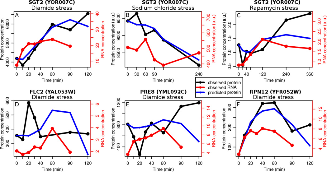
Figure 1. Predictability of protein expression can have several reasons.

The panels show representative RNA and protein time-series profiles of yeast under diamide stress. Panels A–C show one of the genes whose protein levels are predicted well (FDR<30%) for all three data sets. Our model can predict increasing (A), decreasing (B), and more complex profiles (C, F). High predictability is defined by a high Spearman correlation (and FDR<30%) between the observed protein abundance profile (black) and the protein abundance profile predicted with the non-negative linear square fit ODE model (blue). Panels D–E display profiles with a low predictability. In both cases, lack of predictability is likely due to a systematic measurement error in the protein data. Panels E and F show two genes whose biological functions are similar but whose profiles and predictabilities vary. Diamide stress data is presented in absolute abundance units (number of molecules per cell), and the rest of the data is presented in arbitrary units (a.u.) derived from relative abundances.

Clustering

The Pearson distance metric used for clustering is adopted from Eisen et al.¹⁸. The absolute log-transformed protein and mRNA data were first divided by the respective value at time=0 to calculate the profiles of relative concentrations. The profiles were then normalized, such that the distribution of each time-point’s values across all genes was set to mean 0 and variance 1. The R function hclust was used to perform hierarchical clustering, and cutoff was chosen so as to yield the appropriate number of clusters. This number of clusters was chosen based on the average silhouette distances (Figure S3). As the sixth cluster in the Sodium chloride data set would decrease the average silhouette distance (Figure S3) without changing any of our results, we used five clusters for all data sets for consistency.

Parameter landscapes

We used robustness analysis visualized as parameter landscapes to explore the uniqueness of solutions for k_s and k_d. Parameter landscapes display the error for predicting the protein concentration P(t) at a color scale for all k_s and k_d. Aside from reporting the optimal values for k_s and k_d (at 30% FDR, see above), we asked how robust these values are to changes and if other values would provide similarly good predictions of protein concentration changes. The appropriate range of k_s and k_d values was first chosen such that it includes the k_s and k_d values inferred by the time-series ODE model, and the ranges were then broken up into 40 subdivisions equally-spaced on a log scale. For each gene, each of the 1,600 combinations of possible k_s and k_d values was used for calculating the protein time-series profile (Eq. 2). This profile was then compared to the experimentally observed protein time-series profile and scored according to the fraction of variance unexplained (fvu). For visualization, fvu=1.0 was used as the upper cutoff, with all parameter combinations that yield an fvu larger than this cutoff (i.e. when mean square error of the prediction is greater than the variance in the protein data) being represented by the same shade of color.

The parameter landscapes calculated for each gene were then clustered by shape. To do so, the covariance matrix was calculated for each gene from the volume-normalized distribution of differences between the fvu values smaller than 1.0 and the 1.0 fvu cutoff. Then all profiles were hierarchically clustered, again using hclust, with a cutoff chosen to yield 5 clusters (the appropriate number of clusters was chosen manually to yield clusters that are large enough and clearly different). The Foerstner metric was used to define the distances between all pairs of covariance matrices¹⁹. Using covariance matrices, but not the mean or extreme vectors, allows for clustering based on the shape of the contour of good but sub-optimal solutions surrounding the optimal solution rather than absolute values of the optimal parameters. The Foerstner metric is convenient because it is invariant under affine inversions and affine transformations of coordinate systems, thus capturing only the shape and direction of the parameter landscape. We manually examined the clusters to confirm that similar profiles were clustered into the same groups.

Cell strain and culture

For experimental validation, Saccharomyces cerevisiae strain(EY0986 ATCC 201388: MATa his3Δ1 leu2Δ0 met15Δ0 ura3Δ0, SSA4-GFP) expressing the GFP-tagged SSA4 gene was cultivated in YPD medium (2% peptone, 2% glucose, 1% yeast extract) to log phase OD₆₀₀ ~ 0.5. Yeast cells were cultivated as in Gasch et al.¹ to validate the Diamide dataset. Cells were treated with 1.5 mM diamide for 90 min. The length of culture was chosen based on the highest difference of protein expression for Ssa4. To inhibit translation and proteasome degradation, cells were incubated prior to the addition of diamide for 15 min in the presence of 100 µg/ ml cycloheximide (Sigma) or 75 µM of MG-132 (Santa Cruz Biotechnology) at 30 ° C, respectively. After stress induction, cells were immediately collected for immunoblotting analysis.

Western blotting

Cell disruption was performed by agitation with glass beads at 4 °C in standard buffer containing 50 mM Tris-HCl pH 7.5, 150 mM NaCl, 1x Protease inhibitor cocktail set I (EMD). The extract was cleared by centrifugation at 13,000×g for 30 min at 4 °C and protein concentration was determined by Bradford assay (BioRad). Proteins (17 µ g) were transferred to a PVDF membrane and immunoblotting was performed using mouse monoclonal anti-GFP antibody (1:5000, Roche). Rabbit polyclonal anti-GAPDH (1:3000 ab9485) was used as loading control. Anti-mouse and anti-rabbit secondary antibodies conjugated with HRP and ECL prime detection reagents were acquired from GE Life Sciences.

Sequence features analysis

We tested the association between 35 sequence features and prediction quality, synthesis, and degradation rates; references are listed in the Suppl. Table S6. For the analysis of associations with prediction quality, we used the Wilcox on test to compare the distribution of scores for a given sequence feature between the set of well-predicted genes and the same number of genes with the lowest prediction quality scores (i.e. Spearman correlation between observed and predicted profiles). Association with prediction quality was tested with Pearson correlation between the prediction quality scores for all genes with the corresponding scores of a given sequence feature. To analyze associations with rates, the Wilcox on test was used to compare the distribution of the respective feature of the top and the bottom quarter of well-predicted genes with the highest or lowest rates, respectively. The results of all these tests can be found in Supplementary Information (Tables S6 and S7).

An Excel table with the input data, predicted synthesis and degradation rates, figures of predicted protein levels and observed data, and parameter landscapes can be found in the Supplementary Information.

Results

One third of the protein expression profiles are well-modeled

A major result of our study is that, using comparatively simple linear functions with time-constant rates (Eq. 2), approximately one third of all protein expression levels can be well-predicted in their dynamic response to a stimulus and deliver estimates of rates of synthesis and degradation, named k_s and k_d, respectively. This result holds true across three different types of stimuli, namely Diamide, Sodium chloride, and Rapamycin stress, where we predicted 22%, 34%, and 29% of the observed genes, respectively (Table 1). The FDR cutoff is kept relatively high at 30%, as the number of data points within each time series is very small. The finding implies that two-thirds of all genes do not adhere to these rate equations which may be due to several reasons: (i) measurements may be too noisy to produce accurate expression profiles; (ii) synthesis and degradation rates may follow higher-order rate equations or other functions producing complex expression profiles; or (iii) additional regulators of translation and degradation alter the output of the basic rate equations. We detected no significant enrichment in any gene functional category for well- or poorly predicted genes (not shown).

Six genes out of 71 genes present in all three datasets were well-predicted: SGT2, KAR2, OLA1, IMD4, HTS1, ZUO1. SGT2 is a Glutamine-rich cochaperone associated to the endoplasmic reticulum²⁰ and its profiles are shown in Figure 1A–C. As one can see, the model built in each case is highly condition-specific for the different gene expression profiles. However, we also observe some general trends across the three conditions, which we discuss in the following sections. Figure 1 shows examples of genes with high (A–C, F) and low (D, E) predictabilities. Well-predicted profiles often have a monotonically increasing or decreasing shape, such as those for SGT2 in Figure 1A, B, but there are also many examples of well-predicted profiles with more complex behaviors. For example, in Figure 1C SGT2 first decreases in protein concentration, then increases, and finally levels out. Our model is able to capture this behavior. In comparison, aside from noise in the data, low predictability is often associated with drastic expression changes due to reasons other than noise and these are evident from examination of profile clusters (discussed below). Such profiles often look smooth except for two or three consecutive outliers in the protein time-series data, as is shown for FLC2 and PRE8 in Figure 1D, E. These possible outliers may be due to technical artifacts or systematic errors rather than noise.

Some profile shapes can be modeled better than others

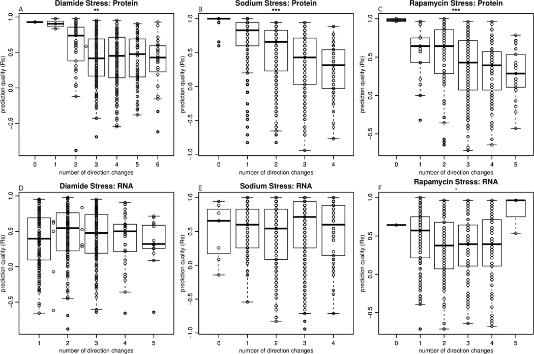
We then investigated how measurement noise affects predictability. With a small number of data points, it is challenging to differentiate between noisy profiles and profiles with complex behaviors that would cause a drastic change at one specific time point due to a biologically relevant mechanism. We assumed that on average, the number of times a protein changes direction in its expression trend (the number of sign changes in the slope of the protein expression curve) is indicative of the level of noise(or the level of orthogonal regulation). Thus, we used the number of changes in sign of expression to assess whether noise is related to predictability, i.e. the Spearman correlation coefficient between observed and predicted protein concentrations (Figure 2). Higher level of noise in protein abundance data, but not the RNA data, is associated with a lower predictability. This is likely due to the fact that RNA expression measurements are less noisy than protein measurements, which is reflected in a lower number RNA profiles with a high number of direction changes. The inverse relationship between noise and predictability is expected, but its magnitude is not large enough to render it the primary or only determinant of predictability. Other proxies of noise, such as absolute mRNA and protein concentrations, did not detect this relationship (Figure S4).

Figure 2. Measurement noise impacts prediction quality.

Each point represents a gene in the Diamide (A, D), Sodium chloride (B, E), or Rapamycin (C, F) stress data set. The y-coordinate of each point represents the prediction quality (measured in Spearman correlation R_s ) of the corresponding gene product, and the x-coordinate represents the number of direction changes in either the protein profile (A–C) or the RNA profile (D–F). The number of direction changes is used as a proxy for noise measurement. Panels A–C show that there is a dependency between prediction quality and noise in the protein profiles (F-test, ** for p<0.01, *** for p<0.001), with more noise corresponding to lower prediction quality. D–F show that there is no such relationship between noise in the RNA profiles and prediction quality. The box in each box plot denotes the interquartile range.

To determine profile shapes that can be well-predicted, we mapped the predictability against the clustered mRNA and protein expression profiles (Figure S5). We found that the number of well-predicted genes is not distributed uniformly across the five expression profile clusters (Pearson chi-squared test, p-value = 5e-11, 1e-09, and 1e-04 for diamide, sodium chloride, and rapamycin stress respectively): some profile shapes are predicted better than others (Table S2). It has previously been reported that only genes where both the RNA and the protein levels are strictly increasing (up-up profiles) can be described well by a correlative model¹⁵. The results for diamide stress and for rapamycin stress confirm that the profile clusters dominated by up-up profiles, i.e. expression profiles in which both mRNA and protein concentrations increase monotonically, are significantly better predicted than other clusters (Table S2, Figures S5, S6). However, in the sodium chloride stress data set, the down-down profiles, where both the RNA and the protein levels are on a steady decline, are modeled better than the other patterns. In sum, the expression profiles dominated by monotonic patterns in protein and RNA expression trend are modeled with the best accuracy, but more complex profiles can also be predicted (e.g. Figures 1C and F).

We examined expression profiles which could not be modeled by our approach, i.e. had very low correlation between predicted and observed protein concentrations. These profiles also share several qualities. For example, these profiles all have one time point for which the median protein profile either has a sudden kink or a trough (Figure 1D, E, Table S2, Figure S6). These kinks are likely to be true signals rather than be due to noise, as an entire group of genes shows the same profiles – but the rate equations cannot model such sudden, singular shift. In the case of diamide stress, the sudden trough in cluster 2 (Figure 1E, Figure S6) may be due to post-translational modification of cysteine-rich proteins (undetected by mass spectrometry) which may or may not be of regulatory nature¹³. In sum, the relationship between profile clusters and predictability is not trivial, and different types of profiles can be predicted using our model. Good predictability can have several sources, e.g. simple expression profile shapes or low measurement noise.

In addition to the condition-dependent features such as profile shape, we tested 35 sequence features (Table S6) for association with prediction quality and for variation in synthesis and degradation rates. The features included amino acid frequencies, molecular weight, codon usage, degradation signals, and intrinsically disordered regions. We found weak association between all three measures of codon usage bias (CAI, CBI, and FOP) and prediction quality (Table S7) for the Diamide and Sodium Chloride data sets, but not for the Rapamycin data set: proteins with optimal codons tend to be better predicted than those with suboptimal codons. The lack of strong associations between sequence features and the results of our model may be due to the fact that the model predictions are highly dependent on experimental conditions, while sequence features are encoded in the genome and do not change between experiments.

The association between sequence features and variation in synthesis and degradation rates was only assessed for the Diamide stress data set, where the predicted rates have biologically realistic values. We found a weak negative correlation between all three measures of codon usage bias used (CAI, CBI, and FOP) and degradation rates, and no significant associations between any either features and synthesis rates.

Synthesis and degradation rates are uncorrelated

We examined general trends in the synthesis and degradation rates that our model extracted. In the Diamide data, absolute protein and mRNA concentrations are reported, while in the Rapamycin and Sodium chloride data relative measurements are reported which relate a protein or mRNA concentration to the concentration at time 0^{1, 12–15}.

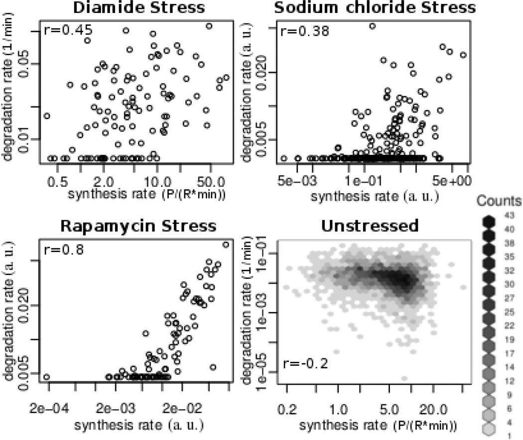
We examined the relationship between synthesis and degradation rates (ks and kd) to test for putative coupling in gene regulation (Figure 3). Coupling would, for example, produce ‘fast responders’ that have higher rates of both protein synthesis and degradation, and ‘slow responders” whose rates are lower. In the Rapamycin dataset, we find a strong correlation between synthesis and degradation rates, suggesting that rapidly produced proteins are also rapidly degraded, and vice versa. In other words, the data suggests that proteins can be ‘fast’ or ‘slow’ in their response, but tend to not be of mixed types. This correlation is only weak in the other datasets. While biologically intriguing, we identified a mathematical explanation of this trend, which suggests that the correlation is due to extensive normalization and is detailed in the Supplement. Because of the weak correlations and the mathematical explanation, we conclude that the synthesis and degradation are largely uncorrelated parameters in these datasets and that there is no evidence for coupling.

Figure 3. Relationship between synthesis and degradation rates.

Each point represents a gene with its rates of protein synthesis or degradation (ks and kd values, respectively). Panels (a)–(c) describe the rates predicted by the ODE model under diamide, sodium chloride, and rapamycin stress respectively, with only the well-predicted genes plotted (FDR=30%). Panel (d) describes measured rates^{16, 17}. We conclude the correlation is spurious and discuss the reasons in the supplement. a.u. – arbitrary units, P – protein concentration, R – RNA concentration, r – Pearson correlation coefficient, t - time.

Parameter landscapes, a measure of prediction uniqueness

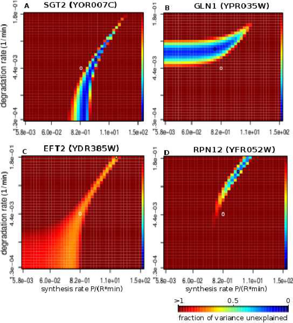
One of the standard techniques in mathematical modeling is the assessment of robustness of the estimated parameters by varying them and comparing the quality of the resulting predictions; we want to assess the uniqueness of one solution for a synthesis or degradation rate compared to a number of possible solutions. From a biological viewpoint, we want to know if tight regulation of one of the two rates is more crucial than the other for recovering the expression profile shape. To that end, we examined the parameter landscapes of the predictions (Figure 4), in which we plot the prediction accuracies onto a map of all possible parameters within a range; prediction accuracies are shown as colors that represent fraction of variance unexplained (Methods). Note that the two measures of prediction quality, Spearman correlation and fraction of variance unexplained, correlate well (Figure S7). Each point in the parameter landscape represents a measure of how well the predicted protein expression profile matches the observed profile. If a rate estimate is unique (with only one possible solution), it would be placed on a steep single ‘mountain’ in the parameter landscape that displays only one area with high prediction quality. In contrast, if a rate estimate delivers good prediction over a range of values, it will be displayed as a broader ‘mountain range’ in the parameter landscape.

Figure 4. Parameter landscapes exploring uniqueness of rate prediction.

Four examples of parameter landscape profiles under diamide stress. A–B show the two most common profiles. Each point represents a certain combination of synthesis rate k_s and degradation rate k_d, and the color represents the quality of the fit that our model produces given these parameters. The quality of fit is given in fraction of variance unexplained (fvu) with darkest blue corresponding to values close to 0 (best fit) and the darkest red representing all fits with fvu greater than or equal to 1.0. The rest of the values fall in between as shown on the color scale on the rightmost column of every heatmap. C presents an example of a gene for which the fit is of approximately the same quality for a wide range of k_s and k_d values, and D shows an example where the solution is rather unique with very few additional solutions. The black circle on each heatmap represents the parameters that optimize the prediction (reported k_s and k_d values), and the white circle marks the center of the heatmap.

We clustered the parameter landscapes for all genes across the three datasets (Figure S8). Figure 4A–B shows the two most common types of profiles found in all three data sets which account for 80–90% of the well-predicted gene parameter landscapes (Figure S8). Figure 4A shows a landscape (a vertical landscape) for SGT2 under diamide stress where varying the degradation rate does not worsen model’s overall prediction capability; but the prediction is very sensitive to changes in synthesis rate. The parameter landscape suggests that the degradation rate could be changed over several orders of magnitude with approximately the same quality of prediction – the regulation of this gene is degradation independent.

Conversely, Figure 4B illustrates an example of a landscape (a horizontal landscape) for glutamine synthetase GLN1 in which the prediction is sensitive to changes in the degradation rate, but not in the synthesis rate. The regulation of GLN1 in response to diamide stress is degradation dependent and synthesis independent. In comparison, Figures 4C and D show examples of parameter landscapes different from these two modes. Thus, for most well-predicted genes the parameter landscapes highlight two types of responses to the stimulus: a gene’s rates may change to address the stress challenge in either a synthesis or a degradation independent manner, only requiring precise change in the respective other rate.

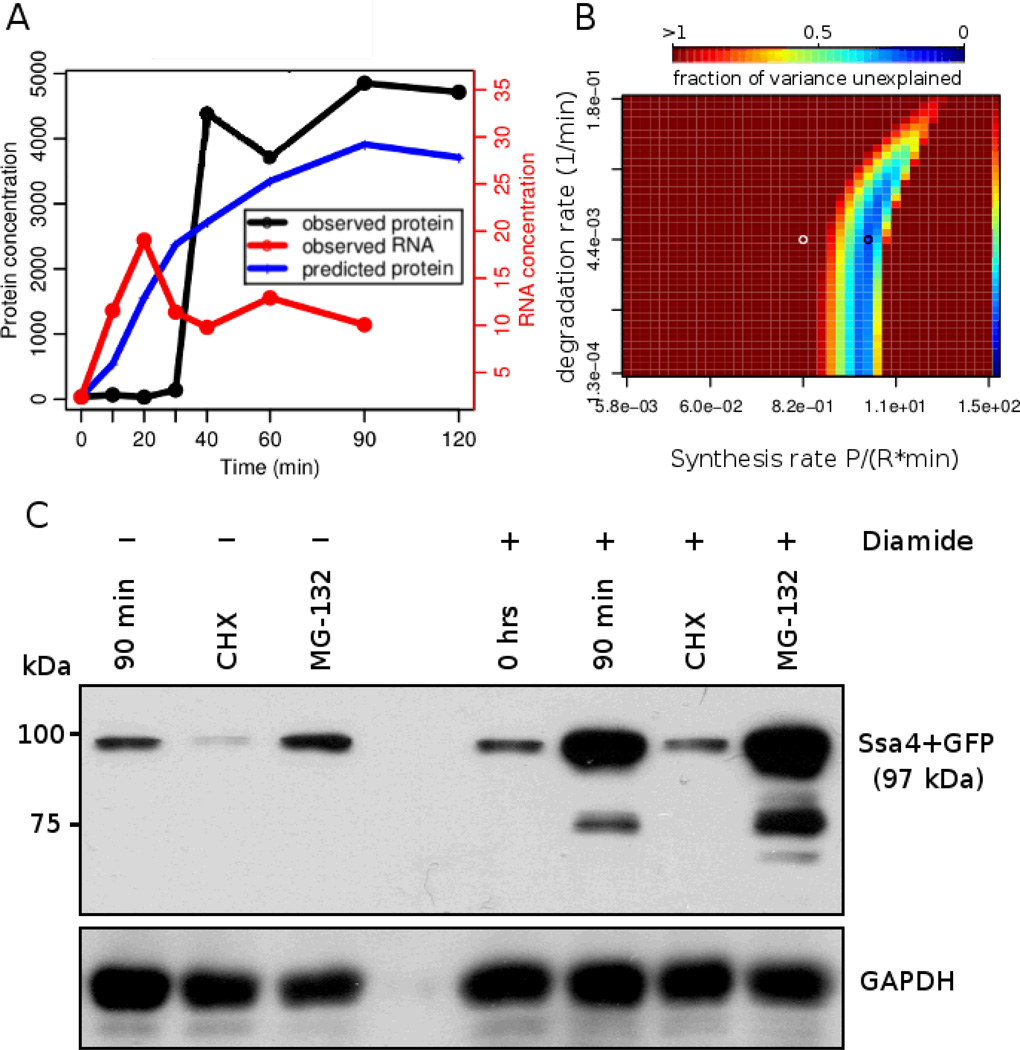
To confirm our prediction that expression regulation depends only on a single rate, we selected the heat shock protein Ssa4, whose vertical parameter landscape suggests degradation-independent regulation. The expression of the Ssa4 protein increases more than 100-fold in response to diamide stress, which allows for a reliable use of western blotting to track abundance changes. Therefore, we cultivated SSA4-GFP tagged cells and subjected them to diamide stress combined with inhibition of protein synthesis or proteasomal degradation using cycloheximide or MG-132, respectively. The results validate our prediction made from the parameter landscape for this gene: the process of attaining the Ssa4 protein expression levels seen under diamide stress is driven by a finely tuned protein synthesis rate, but is largely independent of protein degradation (Figure 5).

Figure 5. Experimental validation of degradation-independent regulation.

Panels A and B show the mRNA and protein expression profile with the predicted protein concentrations and the parameter landscape for the SSA4 gene, respectively. In panel C, the western blot shows the abundance change of the GFP-tagged heat shock protein Ssa4 in cells under diamide stress. After 90 min of 1.5 mM diamide stress, we observe a large increase in Ssa4 abundance, confirming the mass spectrometry results ¹³. Consistent with Ssa4’s degradation-independent mode of regulation, inhibition of protein synthesis with cycloheximide (CHX) substantially affects protein expression under stress, and inhibition of protein degradation with MG-132 has only a minor effect on Ssa4 protein expression levels. GAPDH was used as loading control.

Testing the opposite case of synthesis-independent regulation by western blotting proved to be much more challenging (not shown). Many synthesis-independent well-predicted genes show only small expression fold-changes, rendering them difficult to detect by western blotting. This complication is further enhanced by the intrinsically incomplete proteasome inhibition by MG-132 and the possible action of other proteolytic pathways.

Similar expression profiles have similar parameter landscapes

We explored the dependency between the time-series expression profiles and the predicted synthesis and degradation rates. First we asked whether the genes with similar expression profiles also have similar synthesis and degradation rates, but we found no such dependency (Figure S9). This result can be explained by the different scales of the expression profiles: each cluster has genes with very high and genes with very low expression values. But even in the Rapamycin data, in which the effect of scaling is much reduced due to extensive normalization, we do not observe that genes from the same profile clusters have more similar synthesis and degradation rates than genes from other profile clusters.

We find a relationship between the shape of the expression profiles and of parameter landscapes (Table S3, Chi-squared test p<1e-10): genes are not independently distributed across profile clusters of their parameter landscape clusters. Notably, the intersections of parameter landscape clusters and profile clusters allow us to capture genes that are more strongly enriched in some properties than either clustering alone. Focusing on the largest intersections of clusters helps create a mapping between a gene’s RNA and protein time-series profile and its space of possible synthesis and degradation rates, represented by the gene’s parameter landscape.

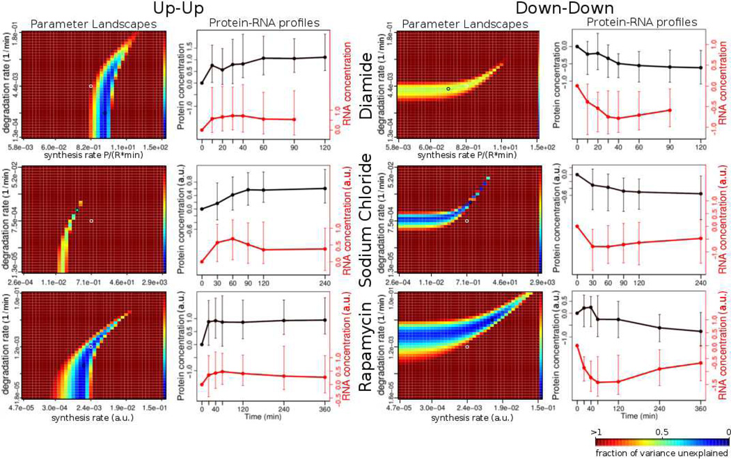
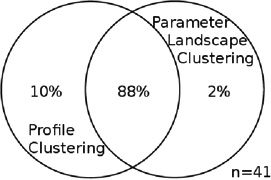
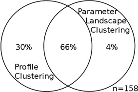
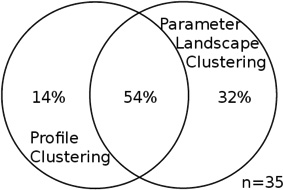
Across the three data sets, the largest intersections (or co-clusters) of profile clusters and parameter landscape clusters occur between the same types of profiles and are shown in Figure 6. We denote these intersections as the up-up and the down-down co-cluster. ‘Up-up’ denotes up-regulation in both mRNA and protein expression along the time course; ‘down-down’ refers to down-regulation in both. Typically, the genes in each of these co-clusters comprise from 50 to 90% of all well-modeled genes in the union of the profile cluster and parameter landscape cluster in question (table 2), indicating a significant similarity between the genes within each of these co-clusters. While there was no significant function enrichment for well- or poorly predicted genes alone (not shown), the genes in the co-clusters are highly enriched in specific functions, and more so than each clustering on its own – suggesting that the co-clustering is a feasible method to extract functionally related genes.

Figure 6. Parameter landscape clusters correspond to profile clusters.

Each heatmap shows a representative example for a cluster of parameter landscapes (see text). The k_s and k_d axes denote the synthesis and the degradation rates, respectively. The color represents the fraction of variance unexplained (fvu), with the bluer hue representing a lower value. The darkest red represents all values of fvu greater than or equal to 1.0. The line graph to the right of each heatmap represents the median profile of the profile cluster that has the largest intersection (by the number of genes in it) with the given cluster of parameter landscapes (see Table 2, Table S3). There are two major types of parameter landscape / profile cluster pairs: the “up-up” (left) and the “down-down” (right). These pairs occur in all three experiments (Diamide, Sodium chloride, Rapamycin), but contain different functional members (Table 2). P – protein concentration; R – RNA concentration, k_s – synthesis rate, k_d – degradation rate.

Table 2. Properties of the most significant intersections between parameter landscape clusters and profile clusters.

For each data set, the two intersections of profile clusters and parameter landscape clusters that contain the largest number of genes are taken; this was either an “up-up” or a “down-down” co-cluster for each data set (see Table S3, Figure S6, S8). Each entry in this table is a Venn diagram that shows the portion of the genes in the intersection of each of those co-clusters as compared to the union of the respective two clusters. The intersection dominates the union, and the overlap is significant. Total number of genes in the union of the two clusters for each co-cluster is specified by n.

	“Up-up” co-cluster	“Down-down” co-cluster
Diamide stress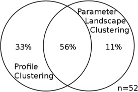
Common gene functions	stress response / antioxidant defense	ribosomal proteins
Sodium chloride stress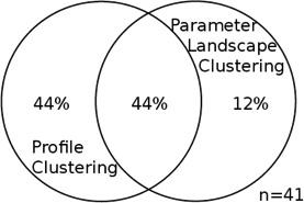
Common gene functions	---	RNA metabolism; ribosomal assembly, bio-genesis and maturation
Rapamycin stress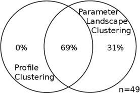
Common gene functions	amino acid synthesis and energy metabolism	ribosomal proteins

The down-down co-clusters from all three stresses are enriched in ribosomal proteins, which is consistent with what we would expect: during different stresses, repression of synthesis of new ribosomes and increased degradation of ribosomes occur, therefore reducing the concentrations of ribosomal proteins^{1, 4, 21–23}. The up-up co-clusters are enriched in different gene functions depending on the stress, e.g. the cluster from the diamide stress is enriched in genes related to stress response and antioxidant defense.

The up-up co-cluster in the Rapamycin stress data set is enriched in amino acid synthesis and energy metabolism²⁴. Furthermore, this comparison of expression profiles and parameter landscapes helps us discover the correct mapping between parameter landscape clusters and their underlying profiles. The up-up co-cluster in Figure 6 shows that independently of the type of stress, the synthesis rates need to be tightly regulated for genes whose transcription and translation are up-regulated, while their degradation rates are not as important to regulate because the resulting protein profiles are robust to large changes in the degradation rates. Conversely, in the down-down co-cluster, we see that the degradation rate is more important to regulate for profiles with decreasing RNA and protein levels, and the synthesis rate can vary a lot without a large effect on the resulting protein time-series profile. In conclusion, the results of co-clustering demonstrate that the general patterns of our model are consistent throughout the three data sets.

Comparing estimated and experimentally determined synthesis and degradation rates

Finally, we evaluate the degree to which the predicted synthesis and degradation rates match experimentally determined rates with respect to biologically plausible, absolute values. Despite extensive literature search, we could not obtain published data on protein translation or degradation rates under stress. The only dataset available was an analysis of H₂O₂ stress in Schizosaccharomyces pombe in which protein, mRNA, and translation efficiency data was collected²⁵. We successfully estimated synthesis and degradation rates from this data that could predict time-dependent expression changes (Table S1), but could not compare values to the ones reported in the publication since the study measured ribosome attachment and density (by ribosome footprinting), but not actual rates.

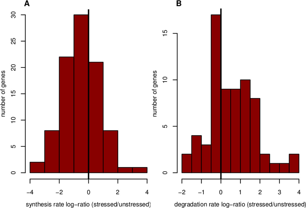
Therefore, we compared our predicted rates to steady state values, which have actual rate estimates available. As explained above, comparison is only possible for the Diamide data set as it contains RNA and protein concentrations with absolute units, i.e. molecules per cell. For the 116 well-predicted genes, we calculated the natural log ratio of the predicted rate under stress to the observed rate under normal conditions^{16, 17}. The log-ratios are distributed normally across the well-predicted genes for both the synthesis and degradation rates (Figure 7). The mean log-ratio for synthesis rates is −0.5±0.1, implying that, on average, the synthesis rates under stress are significantly smaller than the steady-state rates which is expected given a general down-regulation of translation (one-sample t-test, p-value=1e-4). This is also true for the degradation rates (−0.3±0.1). Most (68%) of the predicted synthesis rates range from 1.2 to 13.3 Proteins/(RNA*min), with a median of 4.0 (Table 1), which is very similar to observed synthesis rates which range from 1.7 to 11.4 Proteins/(RNA*min) with a median of 5.8. Most (68%) of the predicted half-lives under stress lie between 16 and 104 minutes with a median of 41 minutes, as compared to observed steady-state half-lives that lie between 20 and 124 minutes, with a median of 45 minutes. These results show that the predicted values fall very well within the range of experimentally measured rates and that even a very simple model can predict realistic rates for a sizable subset of genes in the yeast genome.

Figure 7. Predicted rates are not random.

The histograms show log (base e)-ratios of predicted Diamide stress and observed steady-state synthesis (A) and degradation rates (B). The bars in represent the data points where the stress-induced k_s values are inferred from the well-modeled genes (at FDR 30%). The mean of both of the distributions is significantly different from 0 (one-sample t-test, p=1e-4 and p=3e-4 respectively). The log ratio of 0 is denoted by a black vertical line.

While it is exciting to see that the predicted rates fell well inside the range of experimentally observed values, we did not expect the resolution of the prediction to be precise enough to detect up- or down- regulation of individual genes during the stress response. However, we were able to select some interesting genes to illustrate the potential use of our predicted rates in protein expression regulation. For example, we found three stress-related chaperones (SSA1, AHP1, and CCS1) among the genes with the highest increases in predicted translation rates under stress when compared to the steady-state measurements (Figure S10A). Similarly, we found enzymes of amino acid metabolism (ARG1, GLN1, and THR4) and ribosomal proteins (RPS and RPL genes) to have predicted degradation rates under stress that exceed the steady state degradation rates (Figure S10B).

Discussion

Our analysis shows that the time-dependent protein expression behavior can be predicted for ~30% of the genes in our datasets. To do so, we use first-order rate equations with time invariant rates. This result suggests that a substantial portion of protein expression changes in response to stress, including comparatively complex profile shapes, can be explained without the involvement of additional regulators or parameters. While we confirmed this result in three datasets, future work has to evaluate its generality. For example, when analyzing S. pomberesponding to oxidative stress, only ~10% of the genes can be predicted well using rate equations (Table S1, Supp. Data), which might be due to different technical or biological properties of this dataset.

We investigated several factors in their impact on predictability. There is a weak dependence of predictability on noise in the proteomics data: noisier gene expression patterns tend to be less well predicted than less noisy ones (Figure 2). Genes of similar function can have very different profiles and predictabilities. For example, PRE8 and RPN12 are both highly abundant proteasome subunits, but RPN12 is modeled well under oxidative stress, while PRE8 is not (Figure 1E, F). We investigated the shape of the mRNA and protein expression profiles in their predictability, and identified several shapes with single troughs or peaks that could not be well modeled. For example, a group of oxidative-stress related genes, such as TSA1, SOD2, and PRE8 (Figure 1E) show a marked decrease in concentration at the 20 min time point during diamide stress which prevented predictability. In sum, the presence of additional regulators that may produce complex expression profiles, e.g. with such systematic deviations at specific time points or noisy measurements can explain the lack of predictability in ~70% of the genes.

We also found that use of sub-optimal codons in the open reading frame is associated with a lower prediction quality and a higher degradation rate (Table S7). Sub-optimal codons are interpreted as codons for which the respective tRNAs are comparatively rare, which may result in noisy, non-linear translation. Such scenario in turn breaks the linearity assumption of the finite-difference approximation and can result in a lower prediction quality. Note that this explanation does not affect the magnitude of the synthesis rate, as noisier translation does not imply higher or lower translation rate.

Interestingly, we have found that for the majority of the well predicted genes, the model requires only one of the two rates, synthesis or degradation, to be tightly adjusted, while the other rate is free to accept a wide range of values. We call these regulatory regimes synthesis- or degradation-independent, respectively. In the respective parameter landscapes, this behavior is reflected in a steep ‘peak’ for one rate range, and a wide ‘mountain range’ for the other (Figure 4). For example, most ribosomal subunits are synthesis-independent under diamide stress, which means that it is important for the cell to set degradation of these proteins to a specific rate, but the synthesis rate can assume a number of different values without impacting the overall outcome in the time-dependent protein expression profile. This finding is consistent with translation being down-regulated under oxidative stress^{4, 26}, and presumably the degradation of some ribosomes. In comparison, the regulation of stress response genes such as SOD1 and AHP1, a superoxide dismutase and thiol-specific peroxiredoxin, respectively, is degradation-independentin the diamide experiment. SOD1 and AHP1 play important roles in counteracting the oxidative challenge by deactivating harmful reactive oxygen species²⁷, and thus we expect that their synthesis may be tightly regulated at desired rates while degradation is left to various values. Indeed, the cell has mechanisms in place regulating the transcription and translation of these two proteins^28–30. Most well predicted genes in our dataset are either synthesis- or degradation-independent which provides an economical and time efficient way for the cell to focus regulatory efforts on one mechanism, while neglecting the other, without losing any precision in the desired expression outcome. Figure 5 shows validation for this model at the example of SSA4.

The parameter landscapes describing the robustness of the predictions are linked to gene expression profiles. Proteins following synthesis-independent regulation largely have expression profiles in which both RNA and protein abundances decrease over time, while the degradation-independent proteins mostly increase in RNA and protein levels. Clustering genes according to both regulatory characteristics allows us to extract a group of genes whose behavior is highly similar to each other and that show stronger enrichment in specific gene functions than either characteristic alone. We find that the down-regulated, synthesis-independent genes consist of many ribosomal proteins and proteins involved in RNA metabolism across the three datasets. In contrast, the up-regulated, degradation-independent genes differ in their function enrichments between the stresses. Under diamide stress, this group consists of antioxidant defense genes, while under rapamycin treatment it consists of amino acid metabolism and energy metabolism genes (Table 2).

We compared the predicted translation and degradation rates to experimentally measured values obtained from western-blotting and polysome profiling^{16, 17}. Despite various simplifications and data normalization, our estimated translation rates are highly comparable to the experimentally determined values for cells grown under normal conditions. Likewise, the estimated protein half-lives are very similar on average to steady-state values obtained in independent studies. This result is promising as further optimization of the methods, i.e. including time-dependent rate functions, regulatory interactions between genes, or additional regulators, can lead to new approaches to estimate a so-far understudied area of gene expression regulation, that of protein synthesis and degradation rates. While we focused on analysis of relatively simple profiles, our model also predicted complex behaviors very well (Figure 1C, E, Figure S5) which allows for further insights into complex behaviors. As more and more datasets on absolute mRNA and protein concentrations become available, future work will be able to extend and generalize the predictions to more cases and more complex models. Our pipeline is an important tool for analysis of time-series RNA and protein data collected from a dynamically changing system.

References

- 1.Gasch AP, Spellman PT, Kao CM, Carmel-Harel O, Eisen MB, Storz G, Botstein D, Brown PO. Molecular biology of the cell. 2000;11:4241–4257. doi: 10.1091/mbc.11.12.4241. [DOI] [PMC free article] [PubMed] [Google Scholar]
- 2.Causton HC, Ren B, Koh SS, Harbison CT, Kanin E, Jennings EG, Lee TI, True HL, Lander ES, Young RA. Molecular biology of the cell. 2001;12:323–337. doi: 10.1091/mbc.12.2.323. [DOI] [PMC free article] [PubMed] [Google Scholar]
- 3.Breusing N, Grune T. Biological Chemistry. 2008;389:203–209. doi: 10.1515/BC.2008.029. [DOI] [PubMed] [Google Scholar]
- 4.Shenton D, Smirnova JB, Selley JN, Carroll K, Hubbard SJ, Pavitt GD, Ashe MP, Grant CM. The Journal of biological chemistry. 2006;281:29011–29021. doi: 10.1074/jbc.M601545200. [DOI] [PubMed] [Google Scholar]
- 5.Sideri TC, Stojanovski K, Tuite MF, Grant CM. Proceedings of the National Academy of Sciences of the United States of America. 2010;107:6394–6399. doi: 10.1073/pnas.1000347107. [DOI] [PMC free article] [PubMed] [Google Scholar]
- 6.Davies KJ. IUBMB life. 1999;48:41–47. doi: 10.1080/713803463. [DOI] [PubMed] [Google Scholar]
- 7.Gerashchenko MV, Lobanov AV, Gladyshev VN. Proceedings of the National Academy of Sciences of the United States of America. 2012;109:17394–17399. doi: 10.1073/pnas.1120799109. [DOI] [PMC free article] [PubMed] [Google Scholar]
- 8.Kristensen AR, Gsponer J, Foster LJ. Molecular systems biology. 2013;9:689–689. doi: 10.1038/msb.2013.47. [DOI] [PMC free article] [PubMed] [Google Scholar]
- 9.Schwanhäusser B, Wolf J, Selbach M, Busse D. BioEssays : news and reviews in molecular, cellular and developmental biology. 2013;35:597–601. doi: 10.1002/bies.201300017. [DOI] [PubMed] [Google Scholar]
- 10.Shalem O, Groisman B, Choder M, Dahan O, Pilpel Y. PLoS Genetics. 2011;7:e1002273–e1002273. doi: 10.1371/journal.pgen.1002273. [DOI] [PMC free article] [PubMed] [Google Scholar]
- 11.Lorenz EN. Journal of the Atmospheric Sciences. 1963;20:130–141. [Google Scholar]
- 12.Lu P, Vogel C, Wang R, Yao X, Marcotte EM. Nature biotechnology. 2007;25:117–124. doi: 10.1038/nbt1270. [DOI] [PubMed] [Google Scholar]
- 13.Vogel C, Silva GM, Marcotte EM. Molecular & cellular proteomics : MCP. 2011;10 doi: 10.1074/mcp.M111.009217. [DOI] [PMC free article] [PubMed] [Google Scholar]
- 14.Fournier ML, Paulson A, Pavelka N, Mosley AL, Gaudenz K, Bradford WD, Glynn E, Li H, Sardiu ME, Fleharty B, Seidel C, Florens L, Washburn MP. Molecular & cellular proteomics : MCP. 2010;9:271–284. doi: 10.1074/mcp.M900415-MCP200. [DOI] [PMC free article] [PubMed] [Google Scholar]
- 15.Lee MV, Topper SE, Hubler SL, Hose J, Wenger CD, Coon JJ, Gasch AP. Molecular systems biology. 2011;7 doi: 10.1038/msb.2011.48. [DOI] [PMC free article] [PubMed] [Google Scholar]
- 16.Belle A, Tanay A, Bitincka L, Shamir R, O'Shea EK. Proceedings of the National Academy of Sciences of the United States of America. 2006;103:13004–13009. doi: 10.1073/pnas.0605420103. [DOI] [PMC free article] [PubMed] [Google Scholar]
- 17.Fraser HB, Hirsh AE, Giaever G, Kumm J, Eisen MB. PLoS Biology. 2004;2:e137–e137. doi: 10.1371/journal.pbio.0020137. [DOI] [PMC free article] [PubMed] [Google Scholar]
- 18.Eisen MB, Spellman PT, Brown PO, Botstein D. Proceedings of the National Academy of Sciences of the United States of America. 1998;95:14863–14868. doi: 10.1073/pnas.95.25.14863. [DOI] [PMC free article] [PubMed] [Google Scholar]
- 19.Förstner W, Moonen B. Quo vadis geodesia. 1999;66:113–128. [Google Scholar]
- 20.Kiktev DA, Patterson JC, Muller S, Bariar B, Pan T, Chernoff YO. Molecular and Cellular Biology. 2012;32:4960–4970. doi: 10.1128/MCB.00875-12. [DOI] [PMC free article] [PubMed] [Google Scholar]
- 21.Pestov DG, Shcherbik N. Molecular and Cellular Biology. 2012;32:2135–2144. doi: 10.1128/MCB.06763-11. [DOI] [PMC free article] [PubMed] [Google Scholar]
- 22.Zundel MA, Basturea GN, Deutscher MP. RNA (New York, N.Y.) 2009;15:977–983. doi: 10.1261/rna.1381309. [DOI] [PMC free article] [PubMed] [Google Scholar]
- 23.Powers T, Walter P. Molecular biology of the cell. 1999;10:987–1000. doi: 10.1091/mbc.10.4.987. [DOI] [PMC free article] [PubMed] [Google Scholar]
- 24.Cardenas ME, Cutler NS, Lorenz MC, Di Como CJ, Heitman J. Genes & development. 1999;13:3271–3279. doi: 10.1101/gad.13.24.3271. [DOI] [PMC free article] [PubMed] [Google Scholar]
- 25.Lackner DH, Schmidt MW, Wu S, Wolf DA, Bähler J. Genome biology. 2012;13:R25–R25. doi: 10.1186/gb-2012-13-4-r25. [DOI] [PMC free article] [PubMed] [Google Scholar]
- 26.Grant CM. Antioxidants & redox signaling. 2011;15:191–203. doi: 10.1089/ars.2010.3699. [DOI] [PubMed] [Google Scholar]
- 27.Morano KA, Grant CM, Moye-Rowley WS. Genetics. 2012;190:1157–1195. doi: 10.1534/genetics.111.128033. [DOI] [PMC free article] [PubMed] [Google Scholar]
- 28.Lee J, Spector D, Godon C, Labarre J, Toledano MB. The Journal of biological chemistry. 1999;274:4537–4544. doi: 10.1074/jbc.274.8.4537. [DOI] [PubMed] [Google Scholar]
- 29.Jamieson DJ. Yeast (Chichester, England) 1998;14:1511–1527. doi: 10.1002/(SICI)1097-0061(199812)14:16<1511::AID-YEA356>3.0.CO;2-S. [DOI] [PubMed] [Google Scholar]
- 30.Gralla EB, Thiele DJ, Silar P, Valentine JS. Proceedings of the National Academy of Sciences of the United States of America. 1991;88:8558–8562. doi: 10.1073/pnas.88.19.8558. [DOI] [PMC free article] [PubMed] [Google Scholar]
Associated Data
This section collects any data citations, data availability statements, or supplementary materials included in this article.