

Abstract
The growth patterns of different anatomic structures in the human body vary in terms of growth amount over time, growth rate and growth periods. The oral and pharyngeal structures, also known as vocal tract structures, are housed in the craniofacial complex where the cranium/brain follows a distinct neural growth pattern, and the face follows a distinct somatic or skeletal growth pattern. Thus, it is reasonable to expect the oral and pharyngeal structures to follow a combined or mixed growth pattern. Existing parametric growth models are limited in that they are mainly focused on modeling one particular type of growth pattern. In this paper, we propose a novel composite growth model using neural and somatic baseline curves to fit the combined growth pattern of select vocal tract structures. The method can also determine the overall percent contribution of each of the growth types.
Keywords: growth curves, composite growth model, mixed effects, somatic, neural
1 Introduction
Growth curves of the various structures of the human anatomy are of clinical interest, where the estimated growth curves serve as normative references against which growth is evaluated and atypical growth is identified. Clinical growth charts established by the Center for Disease Control and Prevention (CDC) (www.cdc.gov/growthcharts) for weight, height and head circumference confirm the two major types of growth pattern, namely the somatic and neural growth patterns [5]. These two major growth patterns are depicted in Figure 1. Figure 1 (a) displays the growth of head circumference (HC) that follows a neural growth pattern. Specific characteristics of the neural growth pattern is that there is a period of rapid postnatal growth where about 80% of the adult size is achieved during early childhood; this is then followed by slower steady growth until adulthood. Figures 1 (b) and (c) display body weight and height both of which follow a somatic growth pattern where again much like the neural growth pattern there is rapid postnatal growth. The growth achieved during this early childhood phase, however, is less than 40% of the adult size. This is then followed by a slower growth trend but only up to puberty where there is a second marked accelerated growth period that tapers at about age 15 years for females and about age 18 years for males. These two major growth patterns also characterize the growth of the head-craniofacial complex where the cranium/brain follows a distinct neural growth pattern, and the face follows a distinct somatic or skeletal growth curve.
Figure 1.

Nellhaus head circumference and CDC height and weight growth curves for male and female between 0 and 20 years of age, with a schematic for the proposed growth model (3a)
While head circumference, weight and height follow one particular type of growth pattern, some structures may display developmental changes that cannot be characterized by a single growth pattern. For example, structures housed in the craniofacial complex, such as the vocal tract structures, appear to follow the mixture of both neural and somatic growth patterns [32]. Existing nonlinear human growth models are either lacking of exibility in describing the complex growth pattern of the vocal tract. The empirical evidence so far suggests the vocal tract to have a composite growth model of the form
| (1) |
where Somatic Growth and Neural Growth are the two baseline growth curves obtained from existing growth charts or database. The model (1) fine-tunes to the vocal tract growth pattern since the baseline functions are based on normative growth curves known to represent somatic and neural growth respectively. Computational efficiency of the proposed model is guaranteed relative to nonlinear models because it is a linear combination of known reference curves. Random effects imposed on the linear terms in (1) do not raise computational challenge as nonlinear terms do. The model (1) also allows us to easily determine the contributions of neural and somatic growth by comparing the sum of squared residual between the full model (1) and the reduced models
based on the single component only.
The main contribution of this paper is the introduction of the data driven composite growth model of the form (1) and showing how the model is subsequently used to determine the contributions of different growth types. This is the first paper that models the human growth as a composition of two different growth shapes.
2 Previous Growth Models
As Gasser pointed out [9], efforts in analyzing human growth curves can be broadly divided into fixed and mixed-effects approaches. In this section, we provide a brief survey of notable models in each class.
2.1 Fixed-Effects Models
The model-fitting procedure in the fixed model approach can be either parametric, fully nonparametric or semi-parametric. The parametric models are most commonly used nowadays in studying human growth. Crude nonlinear parametric models were first introduced to fit human growth locally. The Count model [6]
and the Jenss model [11]
were both used for modeling preadolescent height growth. Shohoji and Sasaki [29] used the modified version of Count’s model:
to model individual human height from early childhood to adulthood in Japan. The logistic model for pubertal growth spurt was proposed by Marubini et al. [21] for human height:
Preece and Baines [26] made an attempt at modeling global growth in human height from birth to adulthood by introducing a new family of mathematical functions derived from the differential equation
where h∞ is the adult size and s(t) is a function of time that can be represented by many functions, thus generating a family of growth curves. The most useful models thus generated are
| (2a) |
| (2b) |
where a, b, c, d and e are model parameters. (2a) and (2b) are called the Preece and Baines model 1 (PB1) and model 3 (PB3) respectively. PB1 was shown to be more accurate and robust than PB3.
In an attempt to complement parametric models, Gasser [8] applied a non-parametric model to a longitudinal study of human height growth:
where is the height of subject i measured at age tj, Hi(tj) is the true height and εij are i.i.d. random noises with mean 0 and finite variance . Growth curves for individual subjects were acquired through kernel estimation; the νth derivative of H(t) was estimated by
where {sj} = (tj + tj+1)/2 is an interpolating sequence, b(T) is the smoothing parameter, and the kernel Wν of order (ν, k) satisfies certain moment conditions.
As an alternative to the classical parametric models and nonparametric models, the shape invariant model (SIM), also known as self-modeling nonlinear regression model, was introduced and applied to human growth data by Lawton et al. [20]. The semiparametric approach postulates that a population has a common characteristic function and all the individual growth curves within the population can be modeled by shifting and scaling the characteristic curve. The individual growth curves can be written in the form
where g(t) represents the characteristic function of the population, α and γ are the shifting parameters, and β and δ are the scale parameters. The exponentiation of β and δ is imposed to ensure the positiveness of the parameters and thus avoid identification issues. The characteristic function g(t) can be either parametric or nonparametric. Early applications of SIM included Stützle et al. [30], where a nonlinear function plus a spline function for error correction were used to fit a human growth model.
2.2 Mixed-Effects Models
The fixed-effects model approach of fitting nonlinear curves to individual subjects and then summarizing the parameter estimates for the population is inadequate when we consider the within-subject dependency. Mixed-effects models provide a solution for this problem. For the extensive survey on the mixed-effects model, please refer to Pinheiro and Bates [24]. Ke and Wang proposed a semiparametric mixed-effects model [18]:
where η is a known function defined in terms of the parameter vector ϕi, covariate tij and unknown function f to be estimated via smoothing spline technique; the parameter vector ϕi depends on the fixed-effects vector β (common to all subjects in the population) through the design matrix Ai and a random-effects vector bi (specific the ith subject) through the design matrix Bi; the covariance matrices D and Ri are parametrized by a small number of variance components and correlation coefficients; bi and εi = (εi1, …, εini)′ are mutually independent. Despite its projected exibility in fitting a large class of nonlinear trends, Ke and Wang’s method has computational problems that are not easily accommodated in all cases [7]. A related spline-based mixed-effects SIM model was used by [3] in modeling infant growth. By the log-transformation of the response variable yij (the jth observation of the ith subject), the model is set up to be
where
with unknown covariance matrix Ψ, and
with unknown variance σ2. The characteristic function g(t) is obtained through a cubic smoothing spline with fixed boundary and internal knots, where the boundary knots were chosen to be slightly outside the data range. The model was shown to provide better fit against a form of the Jenss model [11].
2.3 Vocal Tract Growth Modeling
Modeling vocal tract growth is a challenge, in that a good model would require a great deal of fine-tuning towards specific growth pattern such as the adolescent growth-spurt. This requirement rules out a number of classical parametric models confined to describe less complex growth pattens. Polynomial curves and complicated parametric models, as well as nonparametric and semiparametric models, would in theory provide good fits. Vorperian et al. [31] modeled the growth change of various vocal tract portions from birth to adulthood by fourth-order polynomials. Due to great exibility and computational simplicity, polynomial curves in practice remain good candidates in modeling complex growth patterns such as vocal tract growth [17]. However, the main limitation of polynomial curves is downward bending in late adolescence [31].
Barbier et al. used a double-logistic model to fit the growth of the vocal tract from fetus to adulthood [1]. While the double-logistic model provides a close imitation of the vocal tract growth pattern, parameter estimation is nearly impossible for a highly unbalanced data set when random effects are incorporated. Same issues occur with efforts to apply other complex parametric models with random effects. The much more exible spline and kernel smoothing techniques are computationally demanding when the data set is large. On the other hand, the proposed composite growth model will easily accommodates random effects even with large and unbalanced datasets. The patterns specific to vocal tract growth would also be kept by the model at all times.
3 Methods
The term composite growth refers to a linear combination of two different growth types. With the proper choice of the baseline curves, it is possible to model any complex vocal tract growth. For the current study, we use published normative head circumference and weight growth curves that are representative of neural and somatic growth. The neural growth curve N(t) represented by the head circumference growth was obtained by Vorperian et al. [31] from a study conducted by Nellhaus [23], where gender specific population mean growth curves were estimated (Figure 1 (a)). The somatic growth curve S(t) represented by the sex-specific CDC weight growth curves is based upon several national health examination survey datasets taken between the years 1963 and 1994 [5] (Figure 1(b)).
3.1 Mixture Growth Model
Let G(t) represents the measurement of a vocal tract structure at age t. Consider neural N(t) and somatic S(t) curves that characterize two different types of growth. We are interested in modeling G as a linear combination of N and S. Figure 1 (d) shows a schematic of composite growth out of two baseline growth patterns N and S. We fit the following three models simultaneously:
| (3a) |
| (3b) |
| (3c) |
The reduced growth models (3b) and (3c) will be used to determine the contribution of each growth type with respect to the full growth model (3a). The error term ε(t) represents the Gaussian noise N(0, σ2) with unknown variance σ2. The mixed-effects parameters γ’s are given as the sums of fixed-effects terms α’s and random-effects terms β’s:
| (4a) |
| (4b) |
| (4c) |
and the β’s are assumed to follow the distributions
where Ψ, Ψb, Ψc are unknown covariance matrices. The parameter estimation is essentially that of linear mixed-effects models [24].
Since the fixed-effects parameters α’s can be interpreted as the population averages for the corresponding mixed-effects parameters γ’s, we can construct the following formulas to quantify the population growth type based on the respective fixed-effects residual sums of squares R2a, R2b and R2c of the models (3a), (3b) and (3c):
| (5a) |
| (5b) |
where the numerators R2c − R2a and R2b − R2a represent the respective loss of information in models (3c) and (3b) compared with model (3a) due to missing somatic and neural presence, and the denominator R2b + R2c − 2R2a serves to normalize the losses. Note that PS + PN = 100. Formulas (5a) and (5b) are thus associated with natural percentage interpretation of the growth type of a vocal tract portion.
The proposed model (3a) can be interpreted as the scaling of additive characteristic somatic and neural functions from the shape invariant point of view. The variability of individual subjects within the population is incorporated in the random effects of the intercept and scaling factors. The proposed model (3a) has many advantages compared with the existing growth models. (1) Classical models often model a single growth type, whereas the proposed approach models the linear combination of two distinct types of growth. (2) In terms of computation, the proposed model (3a) can be easily implemented when the sample dataset is large, as opposed to the computationally demanding non-parametric and semiparametric mixed-effects models. (3) Since the normative baseline curves S(t) and N(t) originate from sources independent of the dataset, the proposed approach is less biased than estimating the baseline functions and fitting model from a single dataset.
3.2 Simulations
For simulation studies, the baseline longitudinal data was generated using a gender specific fourth-degree polynomial model:
| (6) |
where tij ~ Unif{0, …, 240} follows uniform distribution over integers between 0 and 240, and ; the population coefficients are
and the coefficients varying between subjects follow
These specific coefficients were obtained by fitting the model (6) to our vocal tract length data. The polynomial growth model was previously used to imitate population growth patterns exhibited by the vocal tract length from birth to adulthood (Vorperian et al. [32]). Based on the simulated data, we then fitted and compared the performance of the proposed composite model to the double logistic model.
The signals and noises are assumed to be independent, and their variances and are specified accordingly in the following two separate simulations
Study 1. N = 20, ni ~ Poisson(15), σ1 = 0.02, σ2 = 0.8;
Study 2. N = 50, ni ~ Poisson(10), σ1 = 0.3, σ2 = 0.3.
Data generated in Study 1 are noisier than those generated in Study 2. Figures 3 and 4 show examples of simulated data in Study 1 and 2. One hundred simulations were run in each study and our composite and double logistic models were fitted in each simulation. The results do not differ greatly even if we increase the number of simulations or change the parameters in the model indicative of robustness of our simulation framework.
Figure 3.
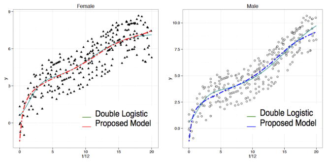
Example of data generated in Study 1 for female and male; green solid and red/blue dashed lines indicate population average fitted curves by double logistic model (7) and proposed model (3a) respectively.
Figure 4.
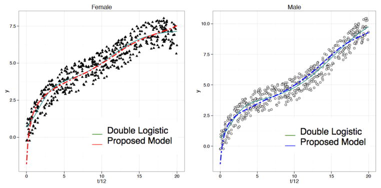
Example of data generated in Study 2 for female and male; green solid and red/blue dashed lines indicate population average fitted curves by double logistic model (7) and proposed model (3a) respectively.
We compared the proposed model (3a, 3b, 3c) against a mixed-effects version of the gender-specific double logistic model used by Barbier et al. [1] for vocal tract growth from fetus to adulthood
| (7) |
where
and Ψp is an unknown covariance matrix. The optimal combinations of random effects were chosen with respect to convergence, correlation and running time. Parameter estimation was handled by the R package lme4.0 [2] for the proposed model (3a) and nlme [25] for the mixed-effects double logistic model.
Table 1 provides a summary of mean squared errors (MSEs) over 100 simulations in Study 1 and 2 and their corresponding standard deviations. The MSEs show that the proposed model (3a) is generally comparable with the mixed-effects double logistic model. The variance between MSEs is also much larger in the double logistic case when more noise is present in the data. The small variance of MSEs in our proposed model (3a) shows its robustness against noise in this type of longitudinal data. Also, Figures 3 and 4 show that the proposed composite model captures the early development of vocal tract type of growth more closely than the double logistic model. The latter is too sensitive to noise to model the sharp growth that characterizes early childhood development.
Table 1.
Mean squared error (MSE) and its one standard deviation for the double logistic and the proposed models (3a) for 100 simulations.
| Study 1 | Double Logistic | Proposed Model |
|---|---|---|
| Female | 0.046 ± 0.013 | 0.047 ± 0.009 |
| Male | 0.031 ± 0.012 | 0.043 ± 0.007 |
| Study 2 | Double Logistic | Proposed Model |
|---|---|---|
| Female | 0.028 ± 0.004 | 0.037 ± 0.005 |
| Male | 0.015 ± 0.004 | 0.041 ± 0.003 |
Note that the data sets generated in both Study 1 and 2 were fairly balanced. The parameter estimation for the mixed-effects double logistic models was relatively easy to handle. However, for many highly unbalanced data sets we have attempted, the mixed-effects double logistic models often failed to converge, whereas the proposed model (3a) converged quickly in every case. The simulation studies suggest that the proposed model (3a) would make a better candidate in modeling unbalanced large-scale longitudinal vocal tract data in practice.
4 Application
We applied the proposed method to model the growth of the four vocal tract portions based on measurements secured from CT images.
4.1 Vocal Tract Data
Measurements were obtained from 771 CT and MRI imaging studies of individuals between birth and 19 years of age. All measurements were made from the midsagittal plane of 419 male and 352 female scans. Some of the individuals had repeated scans and therefore the number of scans were highly unbalanced among subjects. For example, between birth and 19 years, 229 subjects had a single scan. Some subject has up to 10 scans.
Figure 2 displays four variables we used to assess the composite growth model proposed in this paper. The four variables are: (a) VTL, Vocal Tract Length, defined as the curvilinear distance along the midline of the vocal tract starting at the level of the vocal fold (VF) to the intersection with a line drawn tangentially to the lips (L); (b) VT-H, Vocal Tract Horizontal, defined as the horizontal distance form where the VTL ends to the posterior pharyngeal wall (PPW); (c) HP-V, Hyoid Posterior Nasal Spine Vertical, defined as the vertical distance from the posterior nasal spine (PNS) to the anterior-inferior border of the Hyoid bone (H); and (d) LP-V, defined as the vertical distance from the PNS to the larynx at the level of the vocal fold (VF). The abbreviation of the variables is consistent with that used by Vorperian et al. [32].
Figure 2.
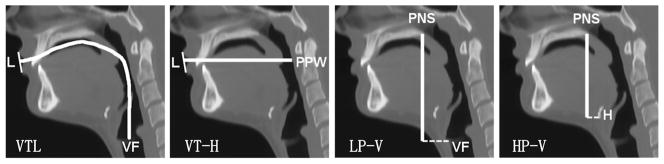
Midsagittal images displaying the anatomic landmarks used for making oral and pharyngeal measurements; the highlighted segments illustrate the actual measurements; left to right: VTL (Vocal Tract Length), VT-H (Vocal Tract Horizontal), LP-V (Larynx-PNS Vertical) and HP-V (Hyoid-PNS Vertical). The landmarks that are used to define the four variables are L (Lips), VF (Vocal Fold), PPW (Posterior Pharyngeal Wall), PNS (Posterior Nasal Spine) and H (Hyoid Bone).
4.2 Results
The mixed-effects models based on (3a), (3b) and (3c) were fitted separately for male and female using the lme4.0 pacakage in R [2]. All combinations of random effects (single, double and full combination) were fitted based on the full fixed-effects model. The Akaike information criterion (AIC) was used as a criterion in comparing the models [3].
Table 2 displays the AICs for all the random-effects combinations of model (3a) for VTL, VT-H, LP-V and HP-V. Chosen combinations have the smallest AICs. For instance, for VTL we should fit random effects on the intercept and the neural growth for female, and fit random effects on the somatic and neural growth for male. The AICs of the chosen models are set in bold face in the table. Figures 5–8 show the estimated population average growth patterns for VTL, VT-H, LP-V and HP-V. All four measurements see a sharp growth spurt between birth and approximately two years of age followed by the second more smooth growth spurt during adolescence.
Table 2.
AIC for mixed-effects models based on (3a); models with the smallest AIC are selected.
| VTL | VT-H | LP-V | HP-V | |||||
|---|---|---|---|---|---|---|---|---|
| Random effects | Female | Male | Female | Male | Female | Male | Female | Male |
| None | 642.83 | 813.10 | 506.57 | 657.98 | 507.85 | 681.29 | 499.05 | 599.04 |
| β0 | 566.98 | 741.95 | 400.17 | 535.41 | 423.11 | 599.75 | 428.09 | 460.43 |
| β1 | 587.06 | 733.06 | 416.65 | 546.23 | 429.87 | 571.95 | 434.32 | 457.23 |
| β2 | 566.46 | 737.34 | 397.55 | 532.95 | 420.11 | 592.68 | 425.38 | 455.78 |
| β0, β1 | 567.39 | 730.53 | 395.14 | 528.70 | 419.23 | 573.69 | 425.52 | 451.03 |
| β0, β2 | 565.27 | 733.25 | 392.52 | 530.22 | 418.51 | 579.42 | 426.05 | 451.36 |
| β1, β2 | 568.57 | 729.75 | 401.55 | 528.51 | 419.52 | 573.51 | 425.67 | 450.93 |
| β0, β1, β2 | 572.44 | 735.75 | 399.91 | 534.51 | 424.78 | 578.01 | 431.51 | 456.93 |
Figure 5.

VTL: population growth curve (left) and rate (right) based on model (3a).
Figure 8.
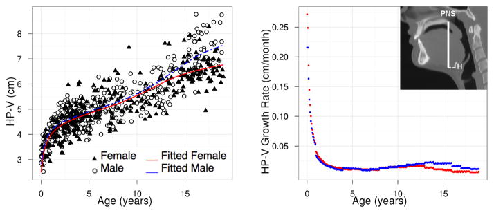
HP-V: population growth curve (left) and rate (right) based on model (3a).
We also compared the performance of the proposed composite growth model to the existing double logistic model. Table 3 shows the comparison between the mean squared errors (MSEs) of the double logistic model and the chosen composite model in Table 2. Our model is in general comparable or outperforms the mixed-effects double logistic model. In fact, the double logistic model fails to converge for the male case of LP-V. Figure 9 shows depiction of VTL population growth trend by the double logistic model and the proposed composite growth model. Although the double logistic model manages to capture the overall growth trend, the sharp growth and plateau that respectively characterize early childhood and late-teen development are not as well depicted as the proposed growth model, particularly for the male curve.
Table 3.
Mean squared errors (MSEs) for the mixed-effects double logistic model (7) and mixed-effects composite growth model (3a) chosen in Table 2 for VTL, VT-H, LP-V and HP-V; NA indicates failure of convergence.
| Female | Double Logistic | Proposed Model |
|---|---|---|
| VTL | 0.111 | 0.058 |
| VT-H | 0.053 | 0.061 |
| LP-V | 0.073 | 0.078 |
| HP-V | 0.083 | 0.086 |
| Male | Double Logistic | Proposed Model |
|---|---|---|
| VTL | 0.226 | 0.239 |
| VT-H | 0.097 | 0.094 |
| LP-V | NA | 0.145 |
| HP-V | 0.092 | 0.091 |
Figure 9.

Population average growth curves of VTL based on mixed-effects double logistic (7) (left) and composite growth model (3a) (right).
Apart from accurate depiction of vocal tract growth trends with computational efficiency, another key contribution of the proposed model is the direct quantification of population growth types. Different structures may have differing contributions of somatic and neural growth (Vorperian et al. [32]). From the residual sum of squares, we can determine the percentage contribution of the growth types. Table 4 shows that the population somatic growth is dominant over neural growth in VTL, LP-V and HP-V for both male and female. For VT-H, population neural growth is shown to dominate over somatic growth for both male and female.
Table 4.
Fixed-effects residual sums of squares R2a, R2b and R2c for models (3a)–(3c), the growth type percent contributions PS and PN, and growth type; in the last column, Somatic/Neural indicates dominance of somatic over neural growth and vice versa.
| Female | R2a | R2b | R2c | PS | PN | Growth type |
|---|---|---|---|---|---|---|
| VTL | 121.74 | 175.93 | 227.32 | 66.08 | 33.92 | Somatic/Neural |
| VT-H | 76.54 | 97.45 | 91.66 | 41.96 | 58.04 | Neural/Somatic |
| LP-V | 80.56 | 92.57 | 135.67 | 82.11 | 17.89 | Somatic/Neural |
| HP-V | 70.08 | 81.62 | 101.16 | 72.93 | 27.07 | Somatic/Neural |
| Male | R2a | R2b | R2c | PS | PN | |
|---|---|---|---|---|---|---|
| VTL | 164.29 | 215.87 | 487.27 | 86.23 | 13.77 | Somaitc/Neural |
| VT-H | 109.76 | 152.79 | 131.48 | 33.55 | 66.45 | Neural/Somatic |
| LP-V | 117.41 | 121.92 | 277.99 | 97.27 | 2.73 | Somatic/Neural |
| HP-V | 101.50 | 109.62 | 184.81 | 91.12 | 8.88 | Somatic/Neural |
Growth velocity is an important growth characteristic that can be easily computed based on a fitted model and visualized. The population growth velocity for a vocal tract portion is approximated from the population average of a model. At a particular age t, we estimate the growth velocity discretely using the finite difference
| (8) |
where Ĝ(t) is the fitted population average of G(t) at age t and Δt is defined to be the difference between t and the later consecutive time point t + Δt. We have taken Δt = 0.1 between ages 0 and 19. Figures 7 and 8 show the growth rate for structures LP-V and HP-V. The growth velocity can be used to visually determine ages of growth spurts. For LP-V and HP-V, the growth spurt occurs earlier for females at around age 12–13 while the the growth spurt occurs later for males at around age 14.
Figure 7.
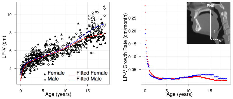
LP-V: population growth curve (left) and rate (right) based on model (3a).
5 Conclusion and Discussion
The proposed method uses existing two normative growth curves in modeling the growth of more complex vocal tract structures as a composition of somatic and neural growth types. Since this is an empirical approach based on available growth curves, the resulting growth model can closely represent documented growth trends. Compared with the traditional parametric growth models, our method is numerically simpler to implement and computationally more efficient. All the traditional models achieve the accuracy in depiction of finer features such as mid-growth spurts by adding parameters and nonlinearity in the model. This adds considerable difficulty in computation for large and highly unbalanced datasets. Algorithms fitting nonlinear models require sensible and stable initial values, which are difficult to obtain when the a model consists of several nonlinear parameters. When random effects are added to the model, convergence might be difficult to obtain due to the unbalanced number of observations between subjects. Our composite growth model, on the other hand, has only linear parameters, which rarely cause divergence when fitting random effects.
The obvious limitation of the proposed model (3a), however, lies with the requirement of distinct baseline growth curves that behave like basis functions in representing more complex growth patterns. If a biological structure does not follow a documented combination of distinct growth trends, our approach may not offer an accurate depiction of the growth. Neither would it be useful when reliable reference growth curves do not exist.
One possible application and extension of the proposed model is toward the landmarked-based morphometric study of the human maxillary complex [10], which is closely related to vocal tract structures in terms of growth characetristics. Given the composite biological structure of the maxillary complex, we can expect that the distances between various landmarks on the complex exhibit composite growth patterns similar to those found in the vocal tract structures. We can therefore model the growth of the human maxillary complex by a system of our proposed models. The fitted models could serve as normative references in medical and dental treatments such as maxillary expansion.
Figure 6.

VT-H: population growth curve (left) and rate (right) based on model (3a).
Acknowledgments
This work was supported, in part, by National Institute on Deafness and Other Communication Disorders Grants R03DC4362 (Anatomic Development of the Vocal Tract: MRI Procedures) and R01 DC6282 (MRI and CT Studies of the Developing Vocal Tract) as well as by National Institute of Child Health and Human Development Core Grant P-30 HD03352, awarded to the Waisman Center. We thank Dr. Meghan M. Cotter for assistance securing CDC data and Michael Kelly for helpful comments.
References
- 1.Barbier G, Boë LJ, Vilain A, Captier G. Vocal tract growth from birth to adulthood, applications for articulatory studies in infants and biomechanical modeling of the vocal apparatus. 9th International Seminar on Speech Production (ISSP 2011); Montreal: Canada. 2011. [Google Scholar]
- 2.Bates D, Maechler M, Bolker B. lme4.0: Linear mixed-effects models using S4 classes. R package version 0.999999-3/r1829. 2013 from http://R-Forge.R-project.org/projects/lme4/
- 3.Beath KJ. Infant growth modeling using a shape invariant model with random effects. Statistics in Mdeicine. 2007;26:2547–2564. doi: 10.1002/sim.2718. [DOI] [PubMed] [Google Scholar]
- 4.Bock RD, Thissen D. Fitting multicomponent models for growth in stature. Proceedings of the 9th International Biometrics Conference; Boston: Biometrics Society; 1976. [Google Scholar]
- 5.Centers for Disease Control and Prevention (CDC). National Center for Health Statistics Clinical Growth Charts. 2000 Retrieved April 11, 2008 from http://www.cdc.gov/growthcharts/
- 6.Count EW. Growth patterns of human physique. Human Biology. 1943;15:151–32. [Google Scholar]
- 7.Elmi A, Ratcliffe SJ, Parry S, Guo W. A B-Spline based semiparametric nonlinear mixed effects model. Journal of Computational and Graphical Statistics. 2011;20(2):492–509. [Google Scholar]
- 8.Gasser T, Müller HG, Köhler W, Molinari L, Prader A. Nonparametric regression analysis of growth curves. The Annals of Statistics. 1984;12(1):210–229. [Google Scholar]
- 9.Gasser T, Seifert B. Comment on “Semiparametric nonlinear mixed-effects models and their applications”. Journal of the American Statistical Association. 2001;96(456):1272–1281. [Google Scholar]
- 10.Heo G, Gamble J, Kim PT. Topological analysis of variance and the maxillary complex. Journal of the American Statistical Association. 2012;107(498):477–492. [Google Scholar]
- 11.Jenss RM, Bayley N. A mathematical method for studying growth in children. Human Biology. 1937;9:556–563. [Google Scholar]
- 12.Jolicoeur P, Pontier J, Pernin MO, Sempe M. A lifetime asymptotic growth curve for human height. Biometrics. 1988;44(4):995–1003. [PubMed] [Google Scholar]
- 13.Jolicoeur P, Pontier J. Population growth and decline: a four-parameter generalization of the logistic curve. Journal of Theoretical Biology. 1989;141(4):563. [Google Scholar]
- 14.Jolicoeur P, Abidi H, Pontier J. Human stature: which growth model. Growth Development and Aging. 1991;55(2):129–132. [PubMed] [Google Scholar]
- 15.Jolicoeur P, Pontier J, Abidi H. Asymptotic models for the longitudinal growth of human stature. American Journal of Human Biology. 1992;4:461–468. doi: 10.1002/ajhb.1310040405. [DOI] [PubMed] [Google Scholar]
- 16.Kanefuji K, Shohoji T. On a growth model of human height. Growth Devolopment and Aging. 1990;54(4):155–165. [PubMed] [Google Scholar]
- 17.Karkach AS. Trajectories and models of individual growth. Demographic Research. 2006;15:347–400. [Google Scholar]
- 18.Ke C, Wang Y. Semiparametric nonlinear mixed-effects models and their applications. Journal of the American Statistical Association. 2001;96 (456):1272–1281. [Google Scholar]
- 19.Koops WJ. Multiphasic growth curve analysis. Growth. 1986;50(2):169–177. [PubMed] [Google Scholar]
- 20.Lawton WH, Sylvestre EA, Maggio MS. Self modeling nonlinear regression. Technometrics. 1972;14(3):513–532. [Google Scholar]
- 21.Marubini E, Resele LF, Barghini G. A comparative fitting of the Gompertz and logistic functions to longitudinal height data during adolescence in girls. Human Biology. 1971;43:237–252. [PubMed] [Google Scholar]
- 22.Marubini E. Human Growth. Vol. 1. Plenum Press; New York: 1978. Mathematical handling of long-term longitudinal data; pp. 209–225. [Google Scholar]
- 23.Nellhaus G. Head circumference from birth to eighteen years: Practical composite international and interracial graphs. Pediatrics. 1968;41:106–114. [PubMed] [Google Scholar]
- 24.Pinheiro J, Bates D. Mixed-effects Models in S and S-PLUS. Springer-Verlag; New York: 2000. [Google Scholar]
- 25.Pinheiro J, Bates D, DebRoy S, Sarkar D the R Development Core Team. nlme: Linear and Nonlinear Mixed Effects Models. R package version 3.1-109. 2013 from http://lme4.r-forge.r-project.org/
- 26.Preece MA, Baines MJ. A new family of mathematical models describing the human growth curve. Annals of Human Biology. 1978;5(1):1–24. doi: 10.1080/03014467800002601. [DOI] [PubMed] [Google Scholar]
- 27.Rao CR. The theory of least squares when the parameters are stochastic and its application to the analysis of growth curves. Biometrika. 1965;52:447–458. [PubMed] [Google Scholar]
- 28.Savageau M. Growth equations: A general equation and a survey of special cases. Mathematical Biosciences. 1980;48:267–278. [Google Scholar]
- 29.Shohoji T, Sasaki H. Individual growth of stature of Japanese. Growth. 1987;51:432–450. [PubMed] [Google Scholar]
- 30.Stützle W, Gasser TH, Molinari L, Largo RH, Prader A, Huber PJ. Shape-invariant modeling of human growth. Annals of Human Biology. 1980;7:507–528. doi: 10.1080/03014468000004641. [DOI] [PubMed] [Google Scholar]
- 31.Vorperian HK, Durtschi RB, Wang S, Chung MK, Zeigert AJ, Gentry LR. Estimating head circumference from imaging studies: an improved method. Academic Radiology. 2007;14:1102–1107. doi: 10.1016/j.acra.2007.05.012. [DOI] [PubMed] [Google Scholar]
- 32.Vorperian HK, Wang S, Chung MK, Schimek EM, Durtschi RB, Kent RD, Ziegert AJ, Gentry LR. Anatomic development of the oral and pharyngeal portions of the vocal tract: an imaging study. Journal of Acoustic Society of America. 2009;125(3):1666–78. doi: 10.1121/1.3075589. [DOI] [PMC free article] [PubMed] [Google Scholar]
- 33.Vorperian HK, Wang S, Schimek EM, Durtschi RB, Kent RD, Gentry LR, Chung MK. Developmental sexual dimorphism of the oral and pharyngeal portions of the vocal tract: an imaging study. Journal of Speech, Language and Hearing Research. 2011;54:995–1010. doi: 10.1044/1092-4388(2010/10-0097). [DOI] [PMC free article] [PubMed] [Google Scholar]
- 34.Wishart J. Growth-rate determinations in nutrition studies with the bacon pig and their analysis. Biometrika. 1938;30:16–28. [Google Scholar]
- 35.Wang Y, Ke C. ASSIST: A suite of S functions implementing spline smoothing techniques. http://www.pstat.ucsb.edu/faculty/yuedong/software.html.