Susceptibility tensor imaging of the kidney and its microstructural underpinnings

Abstract

Purpose

The purpose of this study was to determine whether susceptibility tensor imaging (STI) could overcome limitations of current techniques to detect tubules throughout the kidney.

Methods

Normal mouse kidneys (n=4) were imaged at 9.4T using a 3D gradient multiecho sequence (55-micron isotropic resolution). Phase images from 12 orientations were obtained to compute the susceptibility tensor. Diffusion tensor imaging (DTI) with 12 encoding directions was compared with STI. Tractography was performed to visualize and track the course of tubules with DTI and STI. Confocal microscopy was used to identify which tubular segments of the nephron were detected by DTI and STI.

Results

Diffusion anisotropy was limited to the inner medulla of the kidney. DTI did not find a significant number of coherent tubular tracks in the outer medulla or cortex. With STI, we found strong susceptibility anisotropy and many tracks in the inner and outer medulla, and in limited areas of the cortex.

Conclusion

STI was able to track tubules throughout the kidney, while DTI was limited to the inner medulla. STI provides a novel contrast mechanism related to local tubule microstructure and may offer a powerful method to study the nephron.

Introduction

The major regulatory roles of the renal system, including filtration, homeostasis, and hormonal regulation, depend on the complex, three-dimensional structure of the nephron. The nephron consists of tubular segments including the proximal tubule, intermediate tubule, connecting tubule, and collecting duct, each with its own unique structure. The organization and arrangement of the segment structures are essential to the functions that relate to physiology. The tools available to assess these complex three-dimensional structures in the native tissue, however, are limited. The few tools available, including MRI and CT, have been used to study general renal morphology (1–6). One MR contrast mechanism, diffusion tensor imaging (DTI), has been used to assess the integrity and architecture of tubules in humans (7–12) and in animal models (13–16). In the present study, we applied DTI and found that it was only able to track tubules in the inner medulla (IM) of the mouse kidney. DTI did not find a significant number of coherent tubular tracks in the outer medulla (OM) or cortex (CO). The purpose of this study was to determine whether susceptibility tensor imaging (STI) (17,18) could overcome limitations of current techniques to detect tubules throughout the kidney.

STI is a relatively new MR contrast mechanism based on magnetic susceptibility, which can provide unique structural contrast and detect magnetically anisotropic microstructures (19–22). In the brain, STI shows strong anisotropy in the fiber bundles, which is most likely due to the aligned lipid chains in the myelin sheath surrounding the white matter tracts (23–27). Similar to the neuron in the brain, the nephron in the kidney has a similar tubular structure and parallel organization throughout the organ system. We reasoned that STI would also exhibit strong anisotropy in the nephron tubules.

We used a gradient multiecho (GRME) sequence to obtain STI datasets at shorter acquisition times and higher signal-to-noise ratios (SNRs) compared to a single-echo GRE sequence. These data allowed us to map quantitative susceptibility values and quantify anisotropy of tubules in local renal regions. Apparent magnetic susceptibility (AMS) was plotted as a function of tubule angle to characterize the orientation dependence of susceptibility contrast in the tubules. Tractography was performed to visualize and track the course of tubules; in contrast to DTI, STI was able to detect tracks in the renal CO and OM. We identified the tubular segments of the mouse nephron from confocal images of the same kidney used for MRI. Based on the architecture and organization of these structures, we determined which tubular segments were detected by DTI and STI. We report that STI exhibited strong anisotropy and was able to track tubules throughout the kidney. STI may offer a powerful method to study nephron structure and function that overcomes the limitations of DTI. The methods developed may have broad applications in studies of renal physiology, development, and disease.

Methods

Perfusion and fixation

All animal studies were performed at the Duke Center for In Vivo Microscopy and were approved by the Duke Institutional Animal Use and Care Committee. The protocols adhered to the NIH Guide for the Care and Use of Laboratory Animals. All mice used in this study were C57BL/6 wild type (n=4, 3.5 months old).

Animals were provided with free access to water before organ harvest. Mice were anesthetized with isoflurane, a midline abdominal incision was made, and a catheter was inserted into the heart. Transcardial perfusion fixation was used with inflow to the left ventricle and outflow from the right atrium. The animals were perfused with saline and 0.1% heparin followed by 10% formalin. Both saline and formalin were perfused at 8 ml/min for 5 minutes using a perfusion pump. The renal artery, vein, and ureter were ligated and the kidney was excised from the animal. Kidneys were immersed in 10% formalin overnight and then immersed in 10mM phosphate buffered saline the next day.

The right kidney from each animal was used for imaging (n=4). Kidneys were first fixed without contrast agent and scanned to acquire STI and DTI (48 hours after perfusion). After this imaging session, the kidney was actively stained by immersion in a saline solution of 2.5mM ProHance (Gadoteridol, Bracco Diagnostics Inc., Princeton, NJ) to decrease the T₁ and improve SNR (28). This kidney was then scanned to acquire a contrast-enhanced set of STI and DTI images.

Magnetic resonance imaging (MRI)

Images were acquired on a 9.4T system (400 MHz vertical bore Oxford superconducting magnet) dedicated to magnetic resonance histology, i.e., MRI of tissues at microscopic resolution (29). The system consists of an 89-mm vertical bore magnet controlled by a GE Signa console (Epic 12M5, GE Medical Systems, Milwaukee, WI). Table 1 lists details of the MR imaging protocols. STI was acquired using a 3D GRME pulse sequence. DTI was acquired using a 3D diffusion-weighted spin echo sequence (30). One image was acquired without diffusion weighting and 12 with diffusion weighting at a b-value of 1500 s/mm². Twelve gradient directions were used for DTI and 12 specimen orientations were used for STI. All STI datasets, as well as contrast-enhanced DTI datasets, were acquired using a field of view of 14×14×14 mm³ and a matrix size of 256×256×256, resulting in isotropic resolution of 55×55×55 μm³. Due to the significantly longer T₁, DTI without contrast was acquired at a lower resolution to complete the scan in a reasonable amount of time (16³ mm³ field of view, 110³ matrix, 145³ μm³ resolution). DTI datasets were acquired with a diffusion time (i.e., separation between diffusion gradients) of 17 ms (without contrast agent) and 5.7 ms (with contrast agent), while b-value was maintained at 1500 s/mm². The larger voxel size and longer T₂ relaxation time without contrast agent allowed the choice of longer diffusion time to probe larger tubules. The TR for kidneys without contrast agent was also longer due to their longer T₁ relaxation times (~ 1 s).

Table 1.

Imaging protocols.

	Imaging	Sequence	Dir	FAng (°)	TR (ms)	Echoes (n)	TE1/spacing/TEn (ms)	Acq time per dir (hr)
without Gd	STI	GRME	12	35	200	16	3.4/2.9/46.9	3.6
	DTI	DWSE	12	90/180	2000	1	23.6/−/−	6.7
with Gd	STI	GRME	12	50	50	6	3.4/2.9/17.9	0.9
	DTI	DWSE	12	90/180	100	1	11.8/−/−	1.8

GRME = gradient multiecho, DWSE = diffusion-weighted spin echo, Dir = directions, FAng = flip angle

For MRI acquisitions, the kidney was firmly secured in an acrylic specimen cartridge and immersed in Fomblin (Ausimont USA, Inc., Thorofare, NJ) to limit susceptibility artifacts at the tissue boundary. The cartridge was placed inside a sphere, allowing for an arbitrary specimen orientation inside the coil. The tube and coil holder supported a silver solenoid RF resonator (21-mm diameter, 21-mm length). This coil was designed for STI studies at 9.4 T (Supplemental Fig. 1 in Supplemental Material). A smaller RF resonator (14-mm diameter, 21-mm length) was used for DTI studies, where physical reorientation in a sphere was not necessary.

Multiple echo acquisition

The GRME sequence was used to enhance phase and susceptibility SNR (31). The SNR of a summed multiecho dataset is much higher compared to an optimized single echo dataset for identical sequence parameters (except for TEs). A single echo SNR is optimized when TE equals to T₂^* (see derivation in Supplemental Material). Considering the 16 echoes and measured T₂^* values for the non-contrast enhanced kidney, we found a theoretical SNR gain of 3.01 for a cortical region and 3.32 for a medullary region (Table 2). Using 6 echoes for the contrast-enhanced kidney, we found a theoretical SNR gain of 2.09 for a cortical region and 2.04 for a medullary region (Table 2). These theoretical SNR gains were comparable to experimentally measured gains.

Table 2.

Theoretical SNR gains of the two STI datasets. SNR gain is determined by the ratio of multiecho SNR to single echo SNR at the measured T₂^* value.

	Echoes	TE1/spacing/TEn (ms)		T2* (ms)	SNR gain
STI	16	3.4/2.9/46.9	CO	23.8	3.01
without Gd			MD	34.3	3.32
STI	6	3.4/2.9/17.9	CO	15.5	2.09
with Gd			MD	17.7	2.04

CO = cortex, MD = medullary region

Raw k-space data from the GRME acquisitions were used to reconstruct phase images. Phase images from all echoes were averaged to produce the SNR-enhanced phase image. The phase images of all orientations were used to compute susceptibility tensor (details in next section). In addition, the phase image at each orientation was unwrapped and filtered. The filtered phase was then used to solve an inverse problem to calculate a scalar susceptibility image (20), also known as apparent magnetic susceptibility (AMS). This susceptibility image was normalized by the magnetic field strength and represented in ppm of B₀. In the kidney, phase was assumed to be linearly dependent with TE. TE-dependent susceptibility may indicate non-linear phase due to heterogeneous or compartmentalized tissue microstructure (32). Example magnitude and susceptibility images from the multiecho dataset are shown in Fig. 1 (without contrast). The enhanced magnitude image was produced using the multiecho Fourier domain image contrast (33), shown in Fig. 1B. T₂^* values were computed from the magnitude signal decay curves (Fig. 1C).

Fig. 1.

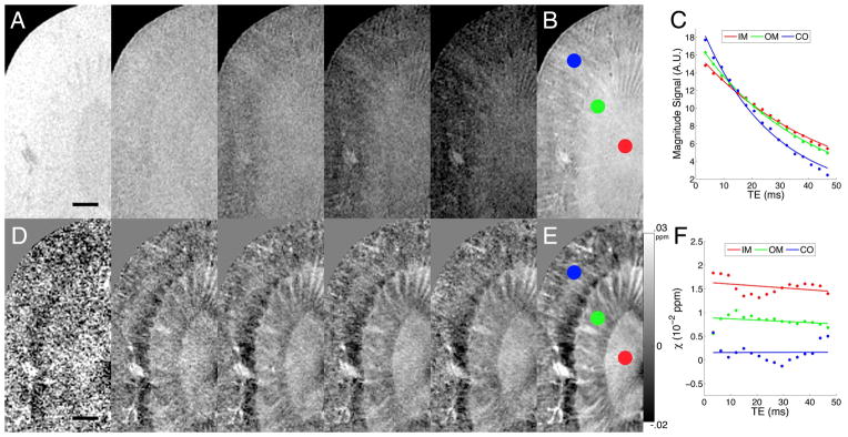
A: Magnitude images at the 1^st (3.4 ms), 4^th (12.1), 7^th (20.8), 10^th, (29.5), and 13^th (38.2) echo. B: Multiecho Fourier domain image contrast (33) was computed from the GRME magnitude dataset. Circles correspond to the IM (red), OM (green), and CO (blue). C: Magnitude signal vs. TE. D: Susceptibility images at the same TEs. E: Enhanced susceptibility image from the multiecho susceptibility dataset. F: Susceptibility vs. TE. Scale bars = 1 mm.

Magnetic susceptibility tensor

The SNR-enhanced phase images at different orientations were registered using rigid body transformation (FMRIB Software Library, http://www.fmrib.ox.ac.uk/fsl) to a common frame of reference (DTI image space). The transformation matrix from registration is used to determine the magnetic field vector in the new image space. Image phase was first unwrapped using a Laplacian-based phase unwrapping algorithm (20,34). Background phase (θ) was removed using a sphere mean value filtering with an initial kernel width of 30 voxels and the kernel width decreasing towards the tissue boundary (35,36). The final phase image (θ) from all echoes was then used for tensor calculation (17,37):

$$\theta =F{T}^{-1}\left\{\frac{1}{3}{\widehat{\mathbf{B}}}_{\mathbf{0}}^{\mathbf{T}}FT\{\chi \}{\widehat{\mathbf{B}}}_{\mathbf{0}}-\mathbf{k}·{\widehat{\mathbf{B}}}_{\mathbf{0}}\frac{{\mathbf{k}}^{\mathbf{T}}FT\{\chi \}{\widehat{\mathbf{B}}}_{\mathbf{0}}}{k^2}\right\}\gamma B_{0}t$$ [1]

where the superscript T represents the transpose operation, B̂₀ is the unit vector of the applied magnetic field, FT is the Fourier transform, FT⁻¹ is the inverse Fourier transform, k is the spatial frequency vector, χ is the second-order (rank 2) susceptibility tensor, γ is the gyromagnetic ratio for water proton, B₀ is the magnitude of the applied magnetic field, and t is the echo time. In our case, each image was already normalized by the echo time before averaging all echoes. There are 6 independent elements for a symmetric rank-2 susceptibility tensor, i.e., χ₁₁, χ₁₂, χ₁₃, χ₂₂, χ₂₃, and χ₃₃ from the 9-element tensor matrix. With multiple measurements of θ at different orientations, susceptibility tensor χ can be solved using a system of linear equations (see Supplemental Material).

Eigenvalue decomposition was performed on the tensor to define the three principal susceptibility values with corresponding eigenvectors. The major eigenvector points in the direction with the most positive (paramagnetic) susceptibility and the minor eigenvector points in the direction with the most negative (diamagnetic) susceptibility. The three eigenvalues were summed to produce the susceptibility trace image.

To determine the relationship between eigenvectors of susceptibility tensors and the underlying tubular orientation, the AMS image was determined for each orientation of the specimen by assuming susceptibility as a scalar in Eq. 1. The relationship between AMS and orientation of a tubular structure is expected to follow (18,26):

$$\mathrm{\Delta }\chi =\mathrm{\Delta }{\chi }_{max}{sin}^2\alpha +\mathrm{\Delta }{\chi }_0$$ [2]

where Δχ is the apparent magnetic susceptibility, Δχ_max is the maximum susceptibility difference, tubule angle (α) is the angle between DTI major eigenvector and magnetic field vector, and Δχ₀ is the baseline isotropic susceptibility difference. It is assumed that the major eigenvector of the diffusion tensor follows the tubular axis in the IM. Tubule angle was computed for each voxel in the IM and grouped into 18 bins. Each bin has a width of 5° (0–5°, 5–10°, …, 85–90°). The AMS dependence on tubule angle was fitted using a least-squares regression.

DTI and STI tractography and quantification

Diffusion fractional anisotropy (FA) was computed following (38). Susceptibility anisotropy (SA) was computed following (18):

$$SA=\frac{{\chi }_3-\frac{{\chi }_2+{\chi }_1}{2}}{{\chi }_3+{\chi }_2+{\chi }_1}$$ [3]

Both FA and SA are in the range of 0 to 1, where 0 is isotropic and 1 is highly anisotropic. DTI and STI tractography were performed using existing algorithms developed for DTI (39). For STI, the vector fields were defined by the minor eigenvector. Both DTI and STI vector fields propagated based on anisotropy measures (FA and SA) between 0.15 and 0.9 and an angle threshold of 60° between neighboring voxels. Tracking was completed in Diffusion Toolkit and TrackVis (http://www.trackvis.org, Martinos Center for Biomedical Imaging, Massachusetts General Hospital). Tracks shorter than 0.38 mm (~7 pixels) were filtered out.

The IM, OM, and CO were segmented to perform measurements in each renal region. Major cortical vessels and medullary vascular bundles were segmented using region growing and thresholding (40) and were then removed to obtain measurements of anisotropy and track statistics of non-vascular origin (segmentation results shown in Supplemental Fig. 2 of Supplemental Material). Metrics determined from the DTI and STI datasets include anisotropy (FA and SA), number of tracks, and track lengths.

Individual kidney images were registered to one common image space in FSL using correlation ratio. Quantitative measurements were conducted for all kidney datasets. Tracking and visualization were derived from the population average of 4 kidneys for each of the following tensor datasets: STI without contrast, DTI without contrast, STI with contrast, and DTI with contrast.

Validation by optical and confocal microscopy

After all MR images were collected, one representative kidney was imaged with 2-photon confocal microscopy and conventional histology. First, the kidney was sectioned near the center coronal plane, cleared using 4M urea (41), and scanned using autofluorescence on a LSM 510 Meta confocal microscope (Carl Zeiss Microscopy, LCC, Thornwood, NY). The laser excitation was two photons at 1000 nm. Emission was detected at 500–550 nm (green channel) and 575–640 nm (magenta channel). Images were acquired at 1.6-μm resolution, at 20-μm depth, and with 14 slices covering 280 μm of tissue using a 20x objective (Zeiss W Plan-Apochromat, NA 1.0). The intact half-sections were then immersed back into 1X (10mM) PBS, embedded in paraffin, and serially sectioned at 5-μm thickness. Sections were stained with Hematoxylin and Eosin (H&E) and Masson’s Trichrome. These slides were scanned using bright field contrast on an Axioskop 2 FS microscope (Carl Zeiss Microscopy, LCC, Thornwood, NY). Images were acquired at 0.65-μm resolution using a 10x objective. Both confocal and optical imaging required tiling to cover the entire kidney. Correction was applied to remove the shading effects and non-uniformities in the tiled images. MR images were manually registered to confocal and optical images to enable comparison.

Results

Apparent magnetic susceptibility (AMS) depends on tubule orientation

Fig. 2 plots AMS in the IM as a function of tubular orientation. AMS was more diamagnetic when tubules were aligned with the magnetic field (0°) and was more paramagnetic when tubules were aligned orthogonal to the magnetic field (90°). Specifically, the AMS displayed a monotonic increase with respect to tubule angle. This trend was observed in the kidney without contrast agent (Fig. 2A–B) and with contrast agent (Fig. 2C–D). These findings suggest that there is a diamagnetic content in the tubule that points along the long axis and also confirm that the STI eigenvector pointing along the tubule axis is the minor eigenvector (most diamagnetic).

Fig. 2.

Plots of AMS vs. tubule angle between DTI major eigenvector and B₀. AMS values are determined in the IM region. Kidney image without contrast agent (A) and corresponding AMS plot (B). Kidney image with contrast agent (C) and corresponding AMS plot (D). AMS (Δχ) is expressed in units of ppb (both y-axis and AMS equation). A and C are susceptibility trace images (registered). Error bar = one standard deviation within each bin.

Comparison between STI and DTI

Fig. 3 shows the 6 elements of the diffusion and susceptibility tensor and includes anisotropy maps (FA and SA). Datasets both with and without contrast agent are shown. The changing diffusion contrast is visible in the IM—indicated by arrows in Fig. 3A and 3E. The alternation of contrast across the susceptibility tensor elements is most noticeable in the IM and OM—indicated by arrows in Fig. 3C and 3G. The changing susceptibility contrast is also apparent in the off-diagonal elements, which indicates susceptibility anisotropy.

Fig. 3.

Tensor arrays in coronal view (A, C, E, G) and anisotropy maps in axial view (B, D, F, H). A–B: DTI (without contrast). C–D: STI (without contrast). E–F: DTI (with contrast). G–H: STI (with contrast). Anisotropy maps include grayscale and color coded maps. White arrows point to the IM in DTI (A, E). Black arrows point to IM and white arrows point to OM in STI (C, G). STI images were inverted to emphasize structures in the renal parenchyma (C, G). Eigenvector axis: red is anteroposterior (AP), green is dorsoventral (DV), and blue is mediolateral (ML). Scale bars = 1mm.

Angles between DTI major eigenvector and STI minor eigenvector were in the range of 10° to 30° in the IM (Supplemental Fig. 3 in Supplemental Material). The angles were much larger in OM and CO—sometimes as large as 90°. This is due to the fact that DTI has poor anisotropy beyond the IM and its major eigenvectors may be more randomly oriented while the minor eigenvectors from STI are still pointing along the tubules. STI results were confirmed by traditional microscopy, which show tubules are generally in the radial direction from CO to IM (see next section).

Fig. 4 compares the population-averaged medullary tracks reconstructed by DTI and STI (with contrast). The tractography color scheme is red for anteroposterior (AP), green for dorsoventral (DV), and blue for mediolateral (ML), which is based on the anatomical directions of the mouse. White arrows point to tracks fanning out in the AP direction and black arrows point to tracks aligned in the ML direction. One yellow arrow points to a few STI tracks pointing towards the DV direction (Fig. 4C). Both DTI and STI tracks point toward the tip of the papilla in the IM. We included a large range of FA values (0.15 to 0.9) and angles (0° to 60°) and observed that DTI tracks were mostly limited to the IM. There were only a few DTI tracks reconstructed in the OM. In comparison, STI tractography detected tubules in both the IM and OM (Fig. 4C–D). Tensor glyphs are also shown in the medullary regions for DTI (Fig. 4B) and STI (Fig. 4D). Tracks of individual kidney datasets are shown in Supplemental Fig. 4 (Supplemental Material).

Fig. 4.

Tractography from DTI (A–B) and STI (C–D) in medullary regions of the kidney (with contrast). A and C: Sagittal view from OM towards papilla tip. B and D: Coronal view. Black arrows point to tracks in ML direction and white arrows point to tracks in AP direction. Yellow arrow indicates additional STI tracks in DV direction (C). DTI tracks overlay b₀ image and STI tracks overlay susceptibility trace image. Insets show tensor glyphs (B, D). White arrows in insets point in the overall direction of glyphs. The major axis of STI glyphs points along the minor eigenvector (largest diamagnetic susceptibility).

Fig. 5 shows the population-averaged cortical and medullary tracks reconstructed by STI (without contrast). Cortical tracks of the entire kidney are shown in a coronal view (Fig. 5A) and a sagittal view (Fig. 5B). Rendering of the OM surface is provided as an anatomical landmark. Medullary tracks are shown in a sagittal view (Fig. 5C) and an axial view (Fig. 5D). Coherent straight tracks in the CO were found in the medial part as well as throughout the kidney (Fig. 5A–B). Very few coherent tracks were reconstructed in the CO by DTI.

Fig. 5.

Additional views of STI tracks (without contrast). A: CO tracks throughout the kidney in a coronal view. B: CO tracks in a sagittal view. Yellow rendering shows the OM surface. C: Sagittal view of medullary tracks traveling down towards IM papilla. D: Axial view of IM tracks.

Table 3 summarizes measurements in the renal regions (IM, OM, and CO) from DTI and STI. Measurements from both non-contrast enhanced and contrast-enhanced datasets are included. Metrics include anisotropy (FA and SA), number of tracks, and track lengths. The IM exhibited strong susceptibility and diffusion anisotropy. The OM exhibited susceptibility anisotropy but weaker diffusion anisotropy (FA<0.2). The CO, on the other hand, exhibited generally weak SA and FA. STI without contrast had a SA>0.2 in the CO. This result confirms the tracks found in Fig. 5. Track number and length were generally greater in STI datasets for all renal regions. Non-contrast enhanced DTI had the fewest number of tracks because of the lower image resolution. All STI metrics (SA, number of tracks, and track lengths) were generally greater in the non-contrast enhanced dataset than in the contrast-enhanced dataset.

Table 3.

Measurements in renal regions from DTI and STI datasets.

		Imaging	IM	OM	CO
Anisotropy (FA or SA)	without Gd	STI	0.39 ± 0.03	0.33 ± 0.01	0.21 ± 0.03
		DTI	0.33 ± 0.01	0.19 ± 0.01	0.15 ± 0.02
	with Gd	STI	0.36 ± 0.02	0.29 ± 0.03	0.19 ± 0.04
		DTI	0.27 ± 0.03	0.17 ± 0.01	0.14 ± 0.01
Number of tracks (102)	without Gd	STI	202 ± 19	497 ± 163	1406 ± 553
		DTI	8 ± 5	4 ± 1	12 ± 6
	with Gd	STI	170 ± 23	23 ± 18	156 ± 123
		DTI	122 ± 79	2 ± 3	16 ± 23
Length (mm)	without Gd	STI	1.1 ± 0.1	0.9 ± 0.1	0.6 ± 0.0
		DTI	1.9 ± 0.7	0.6 ± 0.0	0.6 ± 0.2
	with Gd	STI	1.1 ± 0.1	0.5 ± 0.0	0.5 ± 0.0
		DTI	1.0 ± 0.3	0.4 ± 0.1	0.5 ± 0.0

IM = inner medulla, OM = outer medulla, CO = cortex. Sample size (n=4). Measurements: μ ± σ

Validation by optical and confocal microscopy

Fig. 6 shows the CO, OM, and IM regions identified on optical imaging, confocal microscopy, and MRI. Within the OM, we were able to delineate the inner stripe and outer stripe. The outer stripe was most noticeable in the susceptibility trace image (blue arrow in Fig. 6B) and was not noticeable in the magnitude image (Fig. 6D). Groups of vasa recta were also found in the vascular bundle regions of the inner stripe (black arrows in Fig. 6A–B). The matching of these structures allowed us to confirm alignment of the images and to zoom in on the confocal image to examine the nephron structure corresponding to susceptibility and diffusion anisotropy. We found limited fibrosis in the Mason’s Trichrome histology image, which eliminates collagen as the potential source of susceptibility anisotropy (Fig. 6C). These images also confirmed the accuracy of our segmentation (renal regions, major cortical vessels, and medullary vascular bundles).

Fig. 6.

Image comparison for validation. A: Confocal image. B: Susceptibility trace image. C: Masson’s Trichrome image. D: Magnitude image. Black and white arrows point to corresponding vascular bundles in the inner stripe (IS) of the OM. Blue arrows point to the outer stripe (OS) of the OM. Labeled regions include the CO, OS, IS, and IM. Scale bar = 1mm.

Tubular segments of the nephron were identified from the confocal images (Fig. 7). Standard nomenclature of renal structures is used (42). Scale bars were set at the MRI resolution of 55 μm. Two major nephron types are shown, including the long loop nephron (LLN) associated with the juxtamedullary glomerulus (Fig. 7A–C) and the short loop nephron (SLN) associated with the superficial glomerulus (Fig. 7D–F). The LLN and SLN segments were identified by following the nephrons to the transition point of thin to thick limbs and where the bends occurred. A representative diagram of the nephron is shown in the center of Fig. 7. Overall, the renal tubules are very tortuous and convoluted, which is consistent with previous findings of the mouse kidney (43,44). In the LLN and collecting ducts, there are numerous tortuous tubules, resulting in limited anisotropy from DTI and STI. There are straight segments of the LLN, including the thin limbs in the IM region (Fig. 7A), which resulted in strong anisotropy in both DTI and STI. There are additional straight segments in the LLN, including the thick limbs in the outer stripe and inner stripe regions (Fig. 7A–B); here there was limited diffusion anisotropy and strong susceptibility anisotropy. Coherent structures within a voxel allowed tractography to perform well in DTI and STI.

Fig. 7.

Confocal images of the mouse nephron segments. A, B, C: LLN associated with the juxtamedullary glomerulus (jG). D, E, F: SLN associated with the superficial glomerulus (sG). Straight segments of the LLN: IM descending thin limbs (DTL), IM ascending thin limbs (ATL), inner stripe (IS) medullary thick ascending limbs (mTAL), and outer stripe (OS) distal straight tubules (DST). Tortuous segments of the LLN: OS proximal straight tubule (PST) and IS DTL. The straight portion of the collecting system includes the cortical collecting ducts (CD). All segments of the SLN were tortuous including the OS PST, IS DTL, IS mTAL, and OS DST. F: Left arrow points to the bend of SLN mTAL. Scale bars = 55 μm.

Discussion

Diffusion anisotropy was mostly limited to the IM of the kidney. With STI, we found strong susceptibility anisotropy in the IM and OM, and in limited areas of the CO. This difference was explained by the nephron segments determined from confocal microscopy. One straight segment in the OM (thick limb of the LLN) was detected by STI and not by DTI, thus confirming that DTI and STI anisotropy relied on an entirely different contrast mechanism. Finally, the STI eigenvector pointing along the tubule axis was the minor eigenvector, suggesting that there is a consistent diamagnetic content in the direction of the tubule long axis.

Tensor imaging results explained by the renal tubule

DTI revealed limited anisotropy beyond the IM, while STI showed strong anisotropy in both the IM and OM. As supported by the microscopy results, this differential behavior between DTI and STI is likely due to the diverse microstructures within the IM and OM. These microstructural differences include the tortuosity and the size of the tubules. The mouse renal tubule is especially tortuous, more so than that of larger mammals (45–47). In regions with numerous tortuous nephron segments such as the OM and CO, water diffusion within a voxel (55 μm) would appear isotropic. The other dependence is tubule size. DTI performs well in thin coherent structures where water diffusion is anisotropic. The performance is governed by the average molecular displacement of a Brownian particle in our experiments (48):

$$\overline{x^2}=2Dt$$ [4]

where $\overline{x^2}$ is the mean squared displacement, D is the water diffusion coefficient, and t is the time of diffusion or time between diffusion gradients used for DTI. Given a diffusion coefficient of 2.3×10⁻⁹ m²/s at 25 °C and a diffusion time of 5.7×10⁻³ s, the expected displacement is 5.2 μm (or 8.9 μm without contrast at 17×10⁻³ s diffusion time). In the IM, the thin limbs of the LLN have diameters of approximately 10 μm (49). DTI was able to detect most of these thin tubules with diameters on the lower range. In the OM, there are straight segments such as the LLN thick limbs. These segments have more variable diameters, but are usually thicker and larger than that of the thin limbs, and thus larger than the expected diffusion distance. The thin limbs have limited straight segments in the OM and they also have larger diameters up to 46.7 μm (49). As a result, water diffusion would appear to be isotropic and DTI was not successful in representing the anisotropic structure in the OM. In order to detect such large diameter structures, one would need a diffusion time greater than 470 ms, thus a TE significantly longer than the T₂ of the kidney.

Susceptibility anisotropy, while also expected to be reduced by tortuosity, did not appear to be significantly affected by the size of the tubules. As a result, STI was able to detect the larger straight tubules in the OM. In fact, STI was able to detect these straight segments and many other straight structures throughout the kidney. Even the CO exhibited significant, though reduced, susceptibility anisotropy where the tubules were mostly tortuous and convoluted. STI reconstructed several tracks in the CO (Fig. 5 in Results). In this regard STI exceeded DTI because it is created by a different contrast mechanism based on microstructure and composition and not limited by anisotropic water diffusion.

Biophysical basis of renal STI: cellular components of renal transporting epithelia

There are a number of factors that may contribute to the observed susceptibility anisotropy. These contributing factors may originate from molecular, cellular, and tubular levels.

One potential source is the cellular components of the renal epithelia that compose the tubules. The ordered cellular structure formed by the lipid bilayer found on the plasma membrane and membranes of organelles including the mitochondria will introduce anisotropic susceptibility. Considering the essential features of renal transporting epithelia, there are numerous infoldings of the basement membrane on the basolateral side and an abundance of microvilli of the brush border on the luminal (apical) side. Infoldings and microvilli have been shown to be important for increasing surface areas for fluid absorption and transport and increasing the percentage of cellular lipids in several organs (50–53). The organization of these components are depicted and shown in EM images in Supplemental Fig. 5 (inspired by and adapted with permission from (46,54), see Supplemental Material). These infolding features increase the percentage of lipids pointing in the direction of the tubule. The aligning of the lipids along the axis of the tubule is consistent with the fact that the minor eigenvector of the susceptibility tensor is pointed along the tubules.

The idea of the lipid chain creating susceptibility contrast and anisotropy has been suggested previously (19,55). In the study of susceptibility anisotropy in the brain white matter (19), lipid molecules in the myelin sheath were found to be the main source of anisotropy observed by STI. In the myelinated axons, the long axes of the lipid chains point radially and are perpendicular to the axis of the axon. As a result, the bulk susceptibility of myelinated axons appears to be most diamagnetic in the direction perpendicular to the axons. In other words, the minor eigenvector of the susceptibility tensor is perpendicular to the axons. This is the opposite of what we found in the kidney where the minor eigenvectors were parallel to the tubules. More importantly in both cases, membrane lipids appear to play a significant role.

Within the whole kidney, the most diamagnetic susceptibility was found in the outer stripe of the OM (−8.5 ppb in the STI dataset without contrast and −28.3 ppb in the STI dataset with contrast). Coincidently, the nephron segments in the outer stripe also have the longest microvilli and the most infoldings in the basement membrane, thus increasing the alignment of mitochondria (54,56). These would all contribute to an abundance of lipids and strong diamagnetic susceptibility in the outer stripe.

Besides lipid molecules, there are other macromolecules and cellular contents (extracellular matrix, nucleic acids, and proteins) that may influence the susceptibility in the kidney (22,57–60). Susceptibility anisotropy may also arise due to the compartmentalization of nephron tubules. Further work is needed to determine the relative contributions of these various components. Investigation is also needed to determine how the compartmentalization and composition of the tubules affect the distribution of contrast agent. One way to do that is by using disease or transgenic models with altered molecular and cellular contents.

Technical considerations

One limitation of STI is the requirement of rotating the object and the associated long acquisition time. Twelve orientation datasets were acquired for this study. With improved algorithms to solve the susceptibility tensor equations, the theoretical minimum of 6 orientation datasets can be achieved. Unlike DTI where diffusion anisotropy is sampled by different gradient directions, STI determines susceptibility anisotropy when tissue structure is oriented at different angles with respect to the magnetic field. Automatic reorientation using a goniometer has been demonstrated on samples for electron spin resonance studies (61), and these approaches can be extended to high-resolution imaging of entire specimens. A recent study has demonstrated that STI can be acquired without a physical rotation by sampling the multipole response of the object (62). Applying this technique will be crucial for in vivo imaging. Another limitation of our technique is the structural resolution and specificity. Our voxel size is near the resolution of a single tubule; we are only capable of quantifying the collective susceptibility and anisotropy of tubules within a voxel and not specific tubules or segments. Susceptibility imaging can be sensitive to artifacts that strongly affect magnetic susceptibility. For example, artifacts can arise from air bubble contamination during perfusion and specimen preparation. The kidney area most susceptible to trapping air bubbles is the renal hilum where the fluid content flows through and where the ligation occurs. These susceptibility artifacts also adversely affect DTI. Finally, additional samples and modeling are needed to understand how the tubule compartments and the contrast agent affect susceptibility contrast and anisotropy.

Despite some of the challenges of STI studies, STI offers added benefits over DTI including the detection of straight tubules beyond the IM of the kidney. DTI can potentially detect larger tubules by increasing the diffusion time such that the average displacement of the water molecules is much bigger than the dimensions of the tubules. Such experiments require longer TEs, resulting in significantly lower SNR, which in turn reduces the achievable spatial resolution or requires longer acquisition times. Additionally, STI may have an advantage in detecting subtle changes in the nephron wall structure such as necrosis, where the bilayer lipids are significantly reorganized while the tubule lumen space remains intact. In such cases, susceptibility and susceptibility anisotropy will change significantly while diffusion anisotropy may not. STI can thus be complementary to DTI by providing more sensitive characterization of membrane degradation.

Conclusion

STI is a novel tool to study the nephron structure in the kidney. STI can assess nephron segments where DTI fails, and thus surpasses the current and only MR method to study the renal tubule. The nondestructive nature of MR, the ability to assess the renal microstructures in three dimensions, and the richness of contrasts and quantitative analysis that can be extracted from STI make MRI a promising tool to understand the complex structures of the renal system. The techniques developed in this study can have broad applications in studying the physiology or pathophysiology of the kidney. More importantly, the potential of extending these methods to longitudinal in vivo imaging can answer critical questions about the kidney relating to development and disease progression.

Representative 3D datasets and Supplemental Material are available via CIVMSpace, our method for sharing information with the scientific community <http://www.civm.duhs.duke.edu/lx201210>.

List of abbreviations

Structural nomenclature

AP

anterior-posterior or anteroposterior

CO

cortex

DV

dorsal-ventral or dorsoventral

IM

inner medulla

LLN

long loop nephron

ML

medial-lateral or mediolateral

OM

outer medulla

SLN

short loop nephron

MRI

AMS

apparent magnetic susceptibility

DTI

diffusion tensor imaging

FA

fractional anisotropy

GRME

gradient multiecho

RF

radiofrequency

SA

susceptibility anisotropy

STI

susceptibility tensor imaging

TE

time to echo

TR

time to repetition

Variables

SNR

signal-to-noise ratio

f

frequency offset

M₀

initial magnetization

T₂^*

tissue relaxation time

θ

image phase

T

transpose

B̂₀

unit vector of the applied magnetic field

FT

Fourier transform

FT⁻¹

inverse Fourier transform

k

spatial frequency vector

χ

second-order (rank 2) susceptibility tensor

γ

gyromagnetic ratio for water proton

B₀

magnitude of the applied magnetic field

t

echo time

References

- 1.Beeman SC, Zhang M, Gubhaju L, Wu T, Bertram JF, Frakes DH, Cherry BR, Bennett KM. Measuring glomerular number and size in perfused kidneys using MRI. American journal of physiology Renal physiology. 2011;300(6):F1454–1457. doi: 10.1152/ajprenal.00044.2011. [DOI] [PubMed] [Google Scholar]
- 2.Johnson GA, Cofer GP, Gewalt SL, Hedlund LW. Morphologic phenotyping with magnetic resonance microscopy: the visible mouse. Radiology. 2002;222(3):789–793. doi: 10.1148/radiol.2223010531. [DOI] [PubMed] [Google Scholar]
- 3.Maronpot RR, Sills RC, Johnson GA. Applications of magnetic resonance microscopy. Toxicologic pathology. 2004;32 (Suppl 2):42–48. doi: 10.1080/01926230490451707. [DOI] [PubMed] [Google Scholar]
- 4.Nordsletten DA, Blackett S, Bentley MD, Ritman EL, Smith NP. Structural morphology of renal vasculature. American journal of physiology Heart and circulatory physiology. 2006;291(1):H296–309. doi: 10.1152/ajpheart.00814.2005. [DOI] [PubMed] [Google Scholar]
- 5.Ortiz MC, Garcia-Sanz A, Bentley MD, Fortepiani LA, Garcia-Estan J, Ritman EL, Romero JC, Juncos LA. Microcomputed tomography of kidneys following chronic bile duct ligation. Kidney international. 2000;58(4):1632–1640. doi: 10.1111/j.1523-1755.2000.00324.x. [DOI] [PubMed] [Google Scholar]
- 6.Xie L, Cianciolo RE, Hulette B, Lee HW, Qi Y, Cofer G, Johnson GA. Magnetic resonance histology of age-related nephropathy in the Sprague Dawley rat. Toxicologic pathology. 2012;40(5):764–778. doi: 10.1177/0192623312441408. [DOI] [PMC free article] [PubMed] [Google Scholar]
- 7.Gaudiano C, Clementi V, Busato F, Corcioni B, Ferramosca E, Mandreoli M, Fabbrizio B, Santoro A, Golfieri R. Renal diffusion tensor imaging: is it possible to define the tubular pathway? A case report Magnetic resonance imaging. 2011;29(7):1030–1033. doi: 10.1016/j.mri.2011.02.032. [DOI] [PubMed] [Google Scholar]
- 8.Gurses B, Kilickesmez O, Tasdelen N, Firat Z, Gurmen N. Diffusion tensor imaging of the kidney at 3 Tesla MRI: normative values and repeatability of measurements in healthy volunteers. Diagn Interv Radiol. 2011;17(4):317–322. doi: 10.4261/1305-3825.DIR.3892-10.1. [DOI] [PubMed] [Google Scholar]
- 9.Kataoka M, Kido A, Yamamoto A, Nakamoto Y, Koyama T, Isoda H, Maetani Y, Umeoka S, Tamai K, Saga T, Morisawa N, Mori S, Togashi K. Diffusion tensor imaging of kidneys with respiratory triggering: optimization of parameters to demonstrate anisotropic structures on fraction anisotropy maps. Journal of magnetic resonance imaging: JMRI. 2009;29(3):736–744. doi: 10.1002/jmri.21669. [DOI] [PubMed] [Google Scholar]
- 10.Lanzman RS, Ljimani A, Pentang G, Zgoura P, Zenginli H, Kropil P, Heusch P, Schek J, Miese FR, Blondin D, Antoch G, Wittsack HJ. Kidney transplant: functional assessment with diffusion-tensor MR imaging at 3T. Radiology. 2013;266(1):218–225. doi: 10.1148/radiol.12112522. [DOI] [PubMed] [Google Scholar]
- 11.Notohamiprodjo M, Glaser C, Herrmann KA, Dietrich O, Attenberger UI, Reiser MF, Schoenberg SO, Michaely HJ. Diffusion tensor imaging of the kidney with parallel imaging: initial clinical experience. Investigative radiology. 2008;43(10):677–685. doi: 10.1097/RLI.0b013e31817d14e6. [DOI] [PubMed] [Google Scholar]
- 12.Ries M, Jones RA, Basseau F, Moonen CT, Grenier N. Diffusion tensor MRI of the human kidney. Journal of magnetic resonance imaging: JMRI. 2001;14(1):42–49. doi: 10.1002/jmri.1149. [DOI] [PubMed] [Google Scholar]
- 13.Cheung JS, Fan SJ, Chow AM, Zhang J, Man K, Wu EX. Diffusion tensor imaging of renal ischemia reperfusion injury in an experimental model. NMR in biomedicine. 2010;23(5):496–502. doi: 10.1002/nbm.1486. [DOI] [PubMed] [Google Scholar]
- 14.Hueper K, Hartung D, Gutberlet M, Gueler F, Sann H, Husen B, Wacker F, Reiche D. Magnetic resonance diffusion tensor imaging for evaluation of histopathological changes in a rat model of diabetic nephropathy. Investigative radiology. 2012;47(7):430–437. doi: 10.1097/RLI.0b013e31824f272d. [DOI] [PubMed] [Google Scholar]
- 15.Lu L, Erokwu B, Lee G, Gulani V, Griswold MA, Dell KM, Flask CA. Diffusion-prepared fast imaging with steady-state free precession (DP-FISP): a rapid diffusion MRI technique at 7 T. Magnetic resonance in medicine: official journal of the Society of Magnetic Resonance in Medicine / Society of Magnetic Resonance in Medicine. 2012;68(3):868–873. doi: 10.1002/mrm.23287. [DOI] [PMC free article] [PubMed] [Google Scholar]
- 16.Yang D, Ye Q, Williams DS, Hitchens TK, Ho C. Normal and transplanted rat kidneys: diffusion MR imaging at 7 T. Radiology. 2004;231(3):702–709. doi: 10.1148/radiol.2313021587. [DOI] [PubMed] [Google Scholar]
- 17.Liu C. Susceptibility tensor imaging. Magnetic resonance in medicine: official journal of the Society of Magnetic Resonance in Medicine / Society of Magnetic Resonance in Medicine. 2010;63(6):1471–1477. doi: 10.1002/mrm.22482. [DOI] [PMC free article] [PubMed] [Google Scholar]
- 18.Liu C, Li W, Wu B, Jiang Y, Johnson GA. 3D fiber tractography with susceptibility tensor imaging. NeuroImage. 2012;59(2):1290–1298. doi: 10.1016/j.neuroimage.2011.07.096. [DOI] [PMC free article] [PubMed] [Google Scholar]
- 19.Li W, Wu B, Avram AV, Liu C. Magnetic susceptibility anisotropy of human brain in vivo and its molecular underpinnings. NeuroImage. 2012;59(3):2088–2097. doi: 10.1016/j.neuroimage.2011.10.038. [DOI] [PMC free article] [PubMed] [Google Scholar]
- 20.Li W, Wu B, Liu C. Quantitative susceptibility mapping of human brain reflects spatial variation in tissue composition. NeuroImage. 2011;55(4):1645–1656. doi: 10.1016/j.neuroimage.2010.11.088. [DOI] [PMC free article] [PubMed] [Google Scholar]
- 21.Marques JP, Maddage R, Mlynarik V, Gruetter R. On the origin of the MR image phase contrast: an in vivo MR microscopy study of the rat brain at 14. 1 T. NeuroImage. 2009;46(2):345–352. doi: 10.1016/j.neuroimage.2009.02.023. [DOI] [PubMed] [Google Scholar]
- 22.Lee J, Shmueli K, Fukunaga M, van Gelderen P, Merkle H, Silva AC, Duyn JH. Sensitivity of MRI resonance frequency to the orientation of brain tissue microstructure. Proceedings of the National Academy of Sciences of the United States of America. 2010;107(11):5130–5135. doi: 10.1073/pnas.0910222107. [DOI] [PMC free article] [PubMed] [Google Scholar]
- 23.Liu C, Li W, Johnson GA, Wu B. High-field (9. 4 T) MRI of brain dysmyelination by quantitative mapping of magnetic susceptibility. NeuroImage. 2011;56(3):930–938. doi: 10.1016/j.neuroimage.2011.02.024. [DOI] [PMC free article] [PubMed] [Google Scholar]
- 24.Lee J, Shmueli K, Kang BT, Yao B, Fukunaga M, van Gelderen P, Palumbo S, Bosetti F, Silva AC, Duyn JH. The contribution of myelin to magnetic susceptibility-weighted contrasts in high-field MRI of the brain. NeuroImage. 2012;59(4):3967–3975. doi: 10.1016/j.neuroimage.2011.10.076. [DOI] [PMC free article] [PubMed] [Google Scholar]
- 25.Lodygensky GA, Marques JP, Maddage R, Perroud E, Sizonenko SV, Huppi PS, Gruetter R. In vivo assessment of myelination by phase imaging at high magnetic field. NeuroImage. 2012;59(3):1979–1987. doi: 10.1016/j.neuroimage.2011.09.057. [DOI] [PubMed] [Google Scholar]
- 26.He X, Yablonskiy DA. Biophysical mechanisms of phase contrast in gradient echo MRI. Proceedings of the National Academy of Sciences of the United States of America. 2009;106(32):13558–13563. doi: 10.1073/pnas.0904899106. [DOI] [PMC free article] [PubMed] [Google Scholar]
- 27.Duyn J. MR susceptibility imaging. J Magn Reson. 2013;229:198–207. doi: 10.1016/j.jmr.2012.11.013. [DOI] [PMC free article] [PubMed] [Google Scholar]
- 28.Johnson GA, Cofer GP, Fubara B, Gewalt SL, Hedlund LW, Maronpot RR. Magnetic resonance histology for morphologic phenotyping. Journal of magnetic resonance imaging: JMRI. 2002;16(4):423–429. doi: 10.1002/jmri.10175. [DOI] [PubMed] [Google Scholar]
- 29.Johnson GA, Benveniste H, Black RD, Hedlund LW, Maronpot RR, Smith BR. Histology by magnetic resonance microscopy. Magn Reson Q. 1993;9(1):1–30. [PubMed] [Google Scholar]
- 30.Jiang Y, Johnson GA. Microscopic diffusion tensor imaging of the mouse brain. NeuroImage. 2010;50(2):465–471. doi: 10.1016/j.neuroimage.2009.12.057. [DOI] [PMC free article] [PubMed] [Google Scholar]
- 31.Wu B, Li W, Avram AV, Gho SM, Liu C. Fast and tissue-optimized mapping of magnetic susceptibility and T2* with multi-echo and multi-shot spirals. NeuroImage. 2012;59(1):297–305. doi: 10.1016/j.neuroimage.2011.07.019. [DOI] [PMC free article] [PubMed] [Google Scholar]
- 32.Wharton S, Bowtell R. Fiber orientation-dependent white matter contrast in gradient echo MRI. Proceedings of the National Academy of Sciences of the United States of America. 2012;109(45):18559–18564. doi: 10.1073/pnas.1211075109. [DOI] [PMC free article] [PubMed] [Google Scholar]
- 33.Ali Sharief A, Johnson GA. Enhanced T2 contrast for MR histology of the mouse brain. Magnetic Resonance in Medicine. 2006;56(4):717–725. doi: 10.1002/mrm.21026. [DOI] [PubMed] [Google Scholar]
- 34.Schofield MA, Zhu Y. Fast phase unwrapping algorithm for interferometric applications. Optics letters. 2003;28(14):1194–1196. doi: 10.1364/ol.28.001194. [DOI] [PubMed] [Google Scholar]
- 35.Schweser F, Deistung A, Lehr BW, Reichenbach JR. Quantitative imaging of intrinsic magnetic tissue properties using MRI signal phase: an approach to in vivo brain iron metabolism? NeuroImage. 2011;54(4):2789–2807. doi: 10.1016/j.neuroimage.2010.10.070. [DOI] [PubMed] [Google Scholar]
- 36.Wu B, Li W, Guidon A, Liu C. Whole brain susceptibility mapping using compressed sensing. Magnetic resonance in medicine: official journal of the Society of Magnetic Resonance in Medicine / Society of Magnetic Resonance in Medicine. 2012;67(1):137–147. doi: 10.1002/mrm.23000. [DOI] [PMC free article] [PubMed] [Google Scholar]
- 37.Salomir R, De Senneville BD, Moonen CTW. A fast calculation method for magnetic field inhomogeneity due to an arbitrary distribution of bulk susceptibility. Concept Magn Reson B. 2003;19B(1):26–34. [Google Scholar]
- 38.Basser PJ, Pierpaoli C. Microstructural and physiological features of tissues elucidated by quantitative-diffusion-tensor MRI. J Magn Reson B. 1996;111(3):209–219. doi: 10.1006/jmrb.1996.0086. [DOI] [PubMed] [Google Scholar]
- 39.Basser PJ, Pajevic S, Pierpaoli C, Duda J, Aldroubi A. In vivo fiber tractography using DT-MRI data. Magnetic resonance in medicine: official journal of the Society of Magnetic Resonance in Medicine / Society of Magnetic Resonance in Medicine. 2000;44(4):625–632. doi: 10.1002/1522-2594(200010)44:4<625::aid-mrm17>3.0.co;2-o. [DOI] [PubMed] [Google Scholar]
- 40.Xie L, Sparks MA, Li W, Qi Y, Liu C, Coffman TM, Johnson GA. Quantitative susceptibility mapping of kidney inflammation and fibrosis in type 1 angiotensin receptor-deficient mice. NMR in biomedicine. 2013;26(12):1853–1863. doi: 10.1002/nbm.3039. [DOI] [PMC free article] [PubMed] [Google Scholar]
- 41.Hama H, Kurokawa H, Kawano H, Ando R, Shimogori T, Noda H, Fukami K, Sakaue-Sawano A, Miyawaki A. Scale: a chemical approach for fluorescence imaging and reconstruction of transparent mouse brain. Nature neuroscience. 2011;14(11):1481–1488. doi: 10.1038/nn.2928. [DOI] [PubMed] [Google Scholar]
- 42.Kriz W, Bankir L. A standard nomenclature for structures of the kidney. The Renal Commission of the International Union of Physiological Sciences (IUPS) Kidney international. 1988;33(1):1–7. doi: 10.1038/ki.1988.1. [DOI] [PubMed] [Google Scholar]
- 43.Kriz W, Koepsell H. The structural organization of the mouse kidney. Zeitschrift fur Anatomie und Entwicklungsgeschichte. 1974;144(2):137–163. doi: 10.1007/BF00519771. [DOI] [PubMed] [Google Scholar]
- 44.Zhai XY, Thomsen JS, Birn H, Kristoffersen IB, Andreasen A, Christensen EI. Three-dimensional reconstruction of the mouse nephron. Journal of the American Society of Nephrology: JASN. 2006;17(1):77–88. doi: 10.1681/ASN.2005080796. [DOI] [PubMed] [Google Scholar]
- 45.Cheval L, Pierrat F, Rajerison R, Piquemal D, Doucet A. Of mice and men: divergence of gene expression patterns in kidney. PloS one. 2012;7(10):e46876. doi: 10.1371/journal.pone.0046876. [DOI] [PMC free article] [PubMed] [Google Scholar]
- 46.Christensen EI, Wagner CA, Kaissling B. Comprehensive Physiology. John Wiley & Sons, Inc; 2011. Uriniferous Tubule: Structural and Functional Organization. [DOI] [PubMed] [Google Scholar]
- 47.Lameire NH, Lifschitz MD, Stein JH. Heterogeneity of nephron function. Annual review of physiology. 1977;39:159–184. doi: 10.1146/annurev.ph.39.030177.001111. [DOI] [PubMed] [Google Scholar]
- 48.Einstein A. Investigations on the theory of the Brownian movement. New York: Dover Publications; 1956. p. 119. [Google Scholar]
- 49.Dieterich HJ, Barrett JM, Kriz W, Bulhoff JP. The ultrastructure of the thin loop limbs of the mouse kidney. Anatomy and embryology. 1975;147(1):1–18. doi: 10.1007/BF00317960. [DOI] [PubMed] [Google Scholar]
- 50.Millingt Pf, Critchle Dr. Lipid Composition of Brush Borders of Rat Intestinal Epithelial Cells. Life Sci Pt 1 Physi. 1968;7(15P1):839. [Google Scholar]
- 51.Kawai K, Fujita M, Nakao M. Lipid components of two different regions of an intestinal epithelial cell membrane of mouse. Biochimica et biophysica acta. 1974;369(2):222–233. [PubMed] [Google Scholar]
- 52.Sampaio JL, Gerl MJ, Klose C, Ejsing CS, Beug H, Simons K, Shevchenko A. Membrane lipidome of an epithelial cell line. Proceedings of the National Academy of Sciences of the United States of America. 2011;108(5):1903–1907. doi: 10.1073/pnas.1019267108. [DOI] [PMC free article] [PubMed] [Google Scholar]
- 53.Guan ZZ, Xiao KQ, Zeng XY, Long YG, Cheng YH, Jiang SF, Wang YN. Changed cellular membrane lipid composition and lipid peroxidation of kidney in rats with chronic fluorosis. Archives of toxicology. 2000;74(10):602–608. doi: 10.1007/s002040000177. [DOI] [PubMed] [Google Scholar]
- 54.Maunsbach AB, Christensen EI. Comprehensive Physiology. John Wiley & Sons, Inc; 2010. Functional Ultrastructure of the Proximal Tubule. [Google Scholar]
- 55.Lounila J, Ala-Korpela M, Jokisaari J, Savolainen MJ, Kesaniemi YA. Effects of orientational order and particle size on the NMR line positions of lipoproteins. Physical review letters. 1994;72(25):4049–4052. doi: 10.1103/PhysRevLett.72.4049. [DOI] [PubMed] [Google Scholar]
- 56.Schwartz MM, Venkatachalam MA. Structural differences in thin limbs of Henle: physiological implications. Kidney international. 1974;6(4):193–208. doi: 10.1038/ki.1974.101. [DOI] [PubMed] [Google Scholar]
- 57.Maret G, Schickfus MV, Mayer A, Dransfeld K. Orientation of Nucleic-Acids in High Magnetic-Fields. Physical review letters. 1975;35(6):397–400. [Google Scholar]
- 58.Scholz F, Boroske E, Helfrich W. Magnetic anisotropy of lecithin membranes. A new anisotropy susceptometer Biophysical journal. 1984;45(3):589–592. doi: 10.1016/S0006-3495(84)84196-X. [DOI] [PMC free article] [PubMed] [Google Scholar]
- 59.Torbet J. Fibrin assembly after fibrinopeptide A release in model systems and human plasma studied with magnetic birefringence. The Biochemical journal. 1987;244(3):633–637. doi: 10.1042/bj2440633. [DOI] [PMC free article] [PubMed] [Google Scholar]
- 60.Worcester DL. Structural origins of diamagnetic anisotropy in proteins. Proceedings of the National Academy of Sciences of the United States of America. 1978;75(11):5475–5477. doi: 10.1073/pnas.75.11.5475. [DOI] [PMC free article] [PubMed] [Google Scholar]
- 61.Klette R, Torring JT, Plato M, Mobius K, Bonigk B, Lubitz W. Determination of the G Tensor of the Primary Donor Cation Radical in Single-Crystals of Rhodobacter-Sphaeroides R-26 Reaction Centers by 3-Mm High-Field Epr. J Phys Chem-Us. 1993;97(9):2015–2020. [Google Scholar]
- 62.Liu C, Li W. Imaging neural architecture of the brain based on its multipole magnetic response. NeuroImage. 2013;67:193–202. doi: 10.1016/j.neuroimage.2012.10.050. [DOI] [PMC free article] [PubMed] [Google Scholar]
Associated Data
This section collects any data citations, data availability statements, or supplementary materials included in this article.