Spectral-spatial classification for noninvasive cancer detection using hyperspectral imaging

Abstract.

Early detection of malignant lesions could improve both survival and quality of life of cancer patients. Hyperspectral imaging (HSI) has emerged as a powerful tool for noninvasive cancer detection and diagnosis, with the advantage of avoiding tissue biopsy and providing diagnostic signatures without the need of a contrast agent in real time. We developed a spectral-spatial classification method to distinguish cancer from normal tissue on hyperspectral images. We acquire hyperspectral reflectance images from 450 to 900 nm with a 2-nm increment from tumor-bearing mice. In our animal experiments, the HSI and classification method achieved a sensitivity of 93.7% and a specificity of 91.3%. The preliminary study demonstrated that HSI has the potential to be applied in vivo for noninvasive detection of tumors.

1. Introduction

In 2014, around 1.7 million people will be diagnosed with cancer and 585,720 will die from the disease in the United States.¹ Survival and life quality of the patients correlate directly to the size of the primary tumor at first diagnosis, therefore, early detection of malignant lesions could improve both the incidence and the survival.² Suspicious lesions found through standard screening method should be biopsied for histopathological assessment to make a definitive diagnosis.³ Due to the heterogeneous morphology and visual appearance of the lesions, biopsy diagnosis may not be a representative of the highest pathological grade of a tumor due to the small sampling area.⁴ After biopsies, tissue samples are sectioned and stained. Pathologists then examine the specimens under microscopes and make judgments based on observations of cell morphology and colors of different tissue components. This biopsy procedure is time consuming and invasive. In addition, the interpretation of the histological slides is subjective and inconsistent due to intraobserver and interobserver variations.^3,5

Hyperspectral imaging (HSI) has the potential to improve cancer diagnostics, decrease the use of invasive biopsies, and reduce patient discomfort associated with traditional procedures.⁶ The principle of a wavelength-scanning HSI system consists of illuminating a subject area, spectrally discriminating the reflected light by a dispersive device, and detecting the light reflected from the sample surface onto a two-dimensional (2-D) detector array. By measuring the changes in the reflectance spectrum, structural and biochemical information of tissue can be obtained. The major advantage of HSI is that it is a noninvasive technology that does not require any contrast agent, and it combines wide-field imaging and spectroscopy to simultaneously attain both spatial and spectral information from an object. HSI has been explored for assessment of tissue pathology and pathophysiology based on the spectral characteristics of different tissues^7–9 and has shown potential for noninvasive cancer detection.^10–13

Hyperspectral images, known as hypercubes, are three-dimensional (3D) datasets, ($x$, $y$, $\lambda$) comprising two spatial dimensions $(x,y)$ and one wavelength dimension ($\lambda$). As illustrated in Fig. 1, each plane of the hypercube represents a grayscale image at a particular wavelength, and intensities over all the spectral bands form a spectral signature for each pixel of the hypercube. With the spatial information, the source of each spectrum can be located, which makes it possible to probe the light interactions with pathology. The spectral signature of each pixel can have hundreds of contiguous bands covering the ultraviolet, visible, and near-infrared wavelength range, enabling HSI to identify various pathological conditions.

Fig. 1.

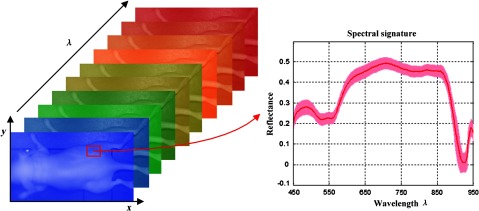
The data structure of a hypercube of hyperspectral imaging (HSI). The red solid line represents the average reflectance spectrum of the rectangular region of the tumor tissue in the mouse, and the color region around the solid line represents the standard deviation of the spectra in the same region.

Hyperspectral images contain rich data. For example, the HSI system employed in this study, which operates in the wavelength range of 450 to 900 nm with a 2-nm interval and an image size of $1040\times 1392\text{\hspace{0.17em}\hspace{0.17em}pixels}$ in the spatial dimension, will generate 1.45 million spectra in one hypercube, each with 226 data points. The quantitative analysis of hyperspectral data is challenging due to the large data volume, including considerable amounts of spectral redundancy in the highly correlated bands, high dimensionality of spectral bands, and high spatial resolution.^12,14 Therefore, machine learning techniques can be applied to mine the vast amounts of data generated in HSI experiments to extract useful diagnostic information and to classify each pixel into cancerous or healthy tissue type.

The traditional classification method for HSI mainly consists of spectral classification and spatial classification. Spectral classification methods only rely on the spectral signature of each pixel in hyperspectral images. For example, Liu et al.¹⁵ proposed a classification method based on the sparse representation of the reflectance spectra for tongue tumor detection from human tongue hyperspectral data of 81 channels from 600 to 1000 nm and achieved an accuracy of 96.5%. Based on the spectral characteristics of tissues, our group used hyperspectral data (450 to 950 nm, 251 channels) and a support vector machine (SVM)-based classifier for prostate tumor detection.¹⁰ Akbari et al. used hyperspectral data (1000 to 2500 nm) for the detection of gastric cancer.¹¹ Spatial classification methods only employed the spatial information for labeling cancerous tissue samples. Masood et al. used hyperspectral images of colon biopsy samples and a single band to classify the sample as normal or cancerous tissues based on the texture feature-circular local binary pattern^16,17 and wavelet texture features.¹⁸ The spectral methods utilized the spectral signature of individual pixels without considering the spatial relationship of neighboring pixels. Spatial-based methods were limited to one spectral band without fully exploiting the spectral information in hyperspectral data. Therefore, how to incorporate spatial and spectral information in a low dimensional space is critical for improving the interpretation and classification of hyperspectral data.

In view of the wealth information available from HSI and the biochemical complexity of tumors, we propose a spectral-spatial classification method that utilizes the entire spectra at each pixel as well as the information from its neighborhood to differentiate between cancerous and normal tissues. Feature extraction and dimension reduction is an important step to extract the most relevant information from the original data and represent that information in a low dimensional space. Dimension reduction methods, such as principal component analysis (PCA),¹⁴ independent component analysis, maximum noise fraction, and sparse matrix transform,^19,20 require spatial rearrangement by vectorizing the 3-D hypercube into two-way data, leading to a loss of spatial information. We propose to preserve the local spectral-spatial structure of the hypercube by tensor computation and modeling. Tensor provides a natural representation for hyperspectral data. In the remote sensing area, tensor modeling has been increasingly utilized for target detection,²¹ denoising,²² dimensionality reduction,^23,24 and classification.^25–28 We extract low-dimensional spectral-spatial features by Tucker tensor decomposition²⁹ and generate probability maps using SVM to indicate how likely it is that each pixel is cancerous. The classification method is generic, which can be applied not only to hyperspectral images but also to other medical images such as MRI and CT images. In this study, we demonstrate the efficacy of HSI in combination with spectral-spatial classification methods for in vivo head and neck cancer detection in an animal model. The experimental design and methods are described in the following sections.

2. Materials

2.1. HSI System

Hyperspectral images were obtained by a wavelength-scanning CRI Maestro (Perkin Elmer Inc., Waltham, Massachusetts) in vivo imaging system. This instrument mainly consists of a flexible fiber-optic lighting system (Cermax-type, 300-Watt, Xenon light source), a solid-state liquid crystal filter (LCTF, bandwidth 20 nm), a spectrally optimized lens, and a 16-bit high-resolution charge-coupled device (CCD). The active light sensitive area of the CCD is 1392 pixels in the horizontal direction and 1040 pixels in the vertical direction. For image acquisition, the wavelength setting can be defined within the range of 450 to 950 nm with 2-nm increments; therefore, the data cube collected was a 3-D array of the size $1040\times 1392\times n$. $n$ is determined by the wavelength range and increments as chosen by the user. The field-of-view (FOV) is from $3.4\times 2.5\mathrm{cm}$ to $10.2\times 7.6\mathrm{cm}$.

2.2. Animal Model

In our experiment, a head and neck tumor xenograft model using HNSCC cell line M4E (doubling rate: $\sim 36\mathrm{h}$) was adopted. The HNSCC cells (M4E) were maintained as a monolayer culture in Dulbecco’s modified Eagle’s medium/F12 medium ($1:1$) supplemented with 10% fetal bovine serum.³⁰ M4Ecells with green fluorescence protein (GFP), which were generated by transfection of pLVTHM vector into M4E cells, were maintained in the same condition as M4E cells. Animal experiments were approved by the Animal Care and Use Committee of Emory University. Female mice aged 4 to 6 weeks were injected with $2\times {10}^6$ M4E cells with GFP on the back of the animals. Hyperspectral images were obtained about 2 weeks post cell injection.

2.3. Reference Image Acquisition

Prior to the animal image acquisition, white reference image cubes were acquired by placing a standard white reference board in the FOV with auto-exposure setting. The dark reference cubes were acquired by keeping the camera shutter closed. These reference images were used to calibrate hyperspectral raw data before image analysis.³¹

2.4. Reflectance Image Acquisition

During the image acquisitions, we first scan the mice using the reflectance mode. Hyperspectral reflectance images were acquired by anesthetizing each mouse with a continuous supply of 2% isoflurane in oxygen. The excitation setting used the interior infrared (800 to 900 nm) excitation and the white light excitation (450 to 800 nm). The acquisition wavelength region for reflectance images was set from 450 to 900 nm with a 2-nm increment. The exposure time was set by the autoexposure configuration. To eliminate the effect of GFP signals in the reflectance images, the emission bands of GFP at 508 and 510 nm were removed in the data preprocessing. Hence, the resultant reflectance images contain 224 spectral bands.

2.5. Fluorescence Image Acquisition

Hyperspectral fluorescence images were subsequently acquired without moving the mouse. The blue excitation light at 455 nm and blue emission filter at 490 nm were used to generate GFP fluorescence images. The exposure time was also set as autoexposure. Tumors show green signals in fluorescence images due to the GFP in tumor cells, and their positions are exactly the same as that in reflectance images. Therefore, GFP fluorescence images can be used as the in vivo gold standard for the classification evaluation of cancer tissue on hyperspectral imaging data.

2.6. Histological Processing

After data acquisitions, mice were sacrificed by cervical dislocation. Tumors were cut horizontally and were then put into formalin. Histological slides were prepared from the tissue specimens for further analysis. The histological diagnosis results were also used to confirm the cancer diagnosis.

3. Methods

In this section, we explain in detail our spectral-spatial classification method. Figure 2(a) illustrates the traditional pixel-wise spectral method which only utilizes spectral information. Vectorization of the 3-D hypercube into a 2-D matrix causes loss of spatial information. PCA is usually applied to reduce data dimensions. Figure 2(b) represents the flowchart for the proposed spectral-spatial method. After the input hypercube is preprocessed, spectral-spatial tensor representation, which conserves the 3-D hypercube structure, is constructed. Tensor decomposition is then performed to extract important features and reduce dimensions. An SVM classifier is then applied to classify each pixel into cancerous or healthy tissues with probability estimates. Any classifier that can provide cancer probability estimates with good classification performance can be applied in this step. Finally, an active contour-based method is performed as a postprocessing step to refine the classification results.

Fig. 2.

The flowcharts of the tissue classification methods. (a) The traditional spectral-based classification method. (b) The proposed spectral-spatial classification method.

3.1. Preprocessing

Hyperspectral data preprocessing aims at removing the effects of the imaging system noise and compensating for geometry-related changes in image brightness. It consists of the following four steps:

• Step 1:
  Reflectance Calibration. Data normalization is required to eliminate the spectral nonuniformity of the illumination and the influence of the dark current. The raw data can be converted into normalized reflectance using the following equation⁸

  $$I_{\text{reflect}}(\lambda )=\frac{I_{\text{raw}}(\lambda )-I_{\text{dark}}(\lambda )}{I_{\text{white}}(\lambda )-I_{\text{dark}}(\lambda )},$$ (1)

  where $I_{\text{reflect}}(\lambda )$ is the calculated normalized reflectance value for each wavelength. $I_{\text{raw}}(\lambda )$ is the intensity value of a sample pixel. $I_{\text{white}}(\lambda )$ and $I_{\text{dark}}(\lambda )$ are the corresponding pixel intensities from the white and dark reference images at the same wavelength as the sample image.
• Step 2:

  Curvature Correction. At the time of imaging, tumors generally protrude outside of the skin and are, therefore, closer to the detector than the normal skin around them. A further normalization has to be applied to compensate for difference in the intensity of light recorded by the camera due to the elevation of tumor tissue. The light intensity changes can be viewed as a function of the distance and the angle between the surface and the detector.³² Two spectra of the same point acquired at two different distances and/or angles will have the same shape but will vary by a constant. By dividing each individual spectrum by a constant calculated as the total reflectance at a given wavelength $\lambda$ removes the distance and angle dependence as well as dependence on an overall magnitude of the spectrum. This normalization step ensures that variations in reflectance spectra are only a function of wavelength, therefore, the differences between cancerous and normal tissues are not affected by the elevation of tumors.

• Step 3:

  Noise Removal. Filters are commonly used for denoising in medical images.^33,34 After the normalization in Steps 1 and 2, the tissue spectra still presents some noise which might be due to the breathing of the mice or small food residuals. Therefore, a median filter is applied to eliminate spectral spikes and to smooth the spectral curves at each pixel, while retaining the variations across different wavelengths.

• Step 4:

  GFP Bands Removal. A GFP signal produces a strong contrast between tumor and normal tissue under blue excitation and may also present a good contrast compared to other spectral bands under white excitation. To eliminate the effect of GFP signals on the cancer detection process, GFP spectral bands, i.e., 508 and 510 nm in our case, are removed from the image cubes before feature extraction.

3.2. Spectral-Spatial Tensor Representation

Tensors are generalization of matrices and vectors. A first-order tensor is a vector, a second-order tensor is a matrix, and tensors of order 3 or higher are called higher-order tensors.³⁵ The order of a tensor is the number of dimensions, which are also known as modes. An $N$-way or $N$’th-order tensor $\underset{\_}{\mathbf{X}}\in {\mathbb{R}}^{J_1\times J_2\times \cdots \times J_N}$ is represented by a multidimensional array with $N$ indices. In this study, hyperspectral data $\underset{\_}{\mathbf{X}}$ is a set of $J_3=224$ images, corresponding to wavelength band from 450 to 900 nm. Each spectral image is composed of $J_1\times J_2$ pixels, with $x_{j_1,j_2,j_3}$ representing the intensity at pixel $(j_1,j_2)$ in spectral band $j_3$.

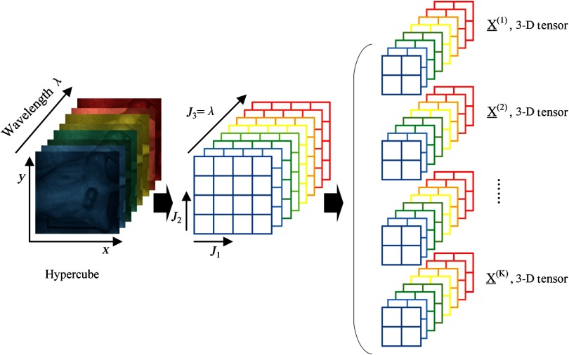
To fully exploit the natural multiway structure of hyperspectral data, we construct a spectral-spatial tensor representation for each pixel by dividing the hypercube $(J_1\times J_2\times J_3)$ into overlapping patches of $3\times 3\times J_3$ dimension. Hence, each pixel is represented by a third-order tensor $\underset{\_}{\mathbf{X}}\in {\mathbb{R}}^{3\times 3\times J_3}$, with two modes representing spatial information, and the third mode for the spectral band. $J_3=\lambda$ represents the number of spectral bands. Figure 3 illustrates the spectral-spatial tensor representation of the hypercube. With the spectral-spatial tensor representation, spectral continuity is represented as the third tensor dimension, whereas spatial information is included as row-column correspondence in the mathematical structure.

Fig. 3.

Spectral-spatial tensor representation of hypercube. Image stack on the left is the hypercube of a tumor-bearing mouse. Images stack in the middle shows that a hypercube ($J_1\times J_2\times J_3$) can be divided into small patches. Image stacks on the right show that each pixel inside a hypercube can be represented by a small patch centered at that pixel. This patch containing information from both the pixel and its neighborhood can be represented in a mathematical form of 3-D tensor.

3.3. Feature Extraction and Dimension Reduction

Tensor decompositions are important tools for feature extraction and dimension reduction because they capture the multiaspect structures of the large scale high dimensional data, with applications in image and signal analysis, neuroscience, chemometrics, etc. Tucker tensor decomposition is a basic model for high-dimensional tensors, which allows effective feature extraction and dimension reduction. An $N$-way Tucker tensor ${\underset{\_}{\mathbf{X}}}^k\in {\mathbb{R}}^{J_1\times J_2\times \cdots \times J_N}$ can be decomposed into a core tensor ${\underset{\_}{\mathbf{G}}}^k\in {\mathbb{R}}^{R_1\times R_2\times \cdots \times R_N}$, multiplied or transformed by a set of component matrices²⁹ ${\mathbf{A}}^{(n)}=({\mathbf{a}}_1^{(n)},{\mathbf{a}}_2^{(n)},\cdots ,{\mathbf{a}}_{R_n}^{(n)})\in {\mathbb{R}}^{J_n\times R_n}(n=\mathrm{1,2},\dots N)$:

$$\begin{gathered} {\underset{\_}{\mathbf{X}}}^k=\sum _{j_1=1}^{R_1}\sum _{j_2=1}^{R_2}\cdots \sum _{j_N=1}^{R_N}{g}_{j_1{j}_2\cdots j_n}({\mathbf{a}}_{j_1}^{(1)}\circ {\mathbf{a}}_{j_2}^{(2)}\circ \cdots {\mathbf{a}}_{j_N}^{(N)})+{\underset{\_}{\epsilon }}^k \\ ={\underset{\_}{\mathbf{G}}}^k\times {{}_1\mathbf{A}}^{(1)}\times {{}_2\mathbf{A}}^{(2)}\cdots \times {{}_N\mathbf{A}}^{(N)}+{\underset{\_}{\epsilon }}^k \\ ={\underset{\_}{\widehat{\mathbf{X}}}}^k+{\underset{\_}{\epsilon }}^k, \end{gathered}$$ (2)

where symbol “$\circ$” represents the outer product, and ${\underset{\_}{\mathbf{G}}}^k\times {{}_1\mathbf{A}}^{(1)}\times {{}_2\mathbf{A}}^{(2)}\cdots \times {{}_N\mathbf{A}}^{(N)}$ denotes the multiplication in all possible modes of a tensor ${\underset{\_}{\mathbf{G}}}^k$ and a set of matrices ${\mathbf{A}}^{(n)}$. In practice, it is common that the core tensor ${\underset{\_}{\mathbf{G}}}^k$ is smaller than the original tensor ${\underset{\_}{\mathbf{X}}}^k$, i.e., $R_N<J_N$. Decomposition of tensor ${\underset{\_}{\mathbf{X}}}^k$ can be seen as a composition of directional bases ${\mathbf{A}}^{(1)},{\mathbf{A}}^{(2)}\cdots {\mathbf{A}}^{(N)}$ in modes $\mathrm{1,2},\dots ,N$, connected through a set of weights contained in ${\underset{\_}{\mathbf{G}}}^k$. The elements in the core tensor ${\underset{\_}{\mathbf{G}}}^k$ represent the features of the sample ${\underset{\_}{\mathbf{G}}}^k$ in the subspace spanned by ${\mathbf{A}}^{(n)}$. Hence, the extracted features are usually in a lower dimension than the original data tensor ${\underset{\_}{\mathbf{X}}}^k$.

We assume that the basis matrices ${\mathbf{A}}^{(n)}=[{\mathbf{a}}_1^{(n)},{\mathbf{a}}_2^{(n)},\cdots ,{\mathbf{a}}_{R_n}^{(n)}]\in {\mathbb{R}}^{J_n\times R_n}(n=\mathrm{1,2},\dots N)$ are common factors for all data tensors. ${\underset{\_}{\hat{\mathbf{X}}}}^k$ is an approximation of ${\underset{\_}{\mathbf{X}}}^k$, and ${\underset{\_}{\epsilon }}^k$ presents the approximation error. Figure 4 illustrates the Tucker decomposition of a three-way tensor. To compute the basis matrices ${\mathbf{A}}^{(n)}$ and the core tensor ${\underset{\_}{\mathbf{G}}}^k$, we concatenate all individual tensors ${\underset{\_}{\mathbf{X}}}^k$ into one $N+1$ order training tensor $\underset{\_}{\mathbf{X}}=\mathrm{cat}({\underset{\_}{\mathbf{X}}}^1,{\underset{\_}{\mathbf{X}}}^2,\cdots ,{\underset{\_}{\mathbf{X}}}^K,N+1)\in {\mathbb{R}}^{J_1\times J_2\times \cdots \times J_N\times J_{N+1}}$ with $J_{N+1}=K$ and perform Tucker-$N$ decomposition.²⁹ The sample tensors ${\underset{\_}{\mathbf{X}}}^k$ can be obtained from the concatenated tensor by fixing the ($N+1$)’th index at a value $k$ and the individual features can be extracted from the core tensor ${\underset{\_}{\mathbf{G}}}^k$ by fixing the ($N+1$)’th index as $k$. In the case of hyperspectral data, the core tensor connects two spatial modes with one spectral mode of the hypercube. Hence, the extracted features simultaneously contain the spectral-spatial profile of tissues in the hyperspectral data ${\underset{\_}{\mathbf{X}}}^k$.

Fig. 4.

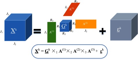
Tucker decomposition of a three-way tensor ${\underset{\_}{\mathbf{X}}}^k$. Decomposition of tensor ${\underset{\_}{\mathbf{X}}}^k$ can be seen as a multiplication in all possible modes of a core tensor ${\underset{\_}{\mathbf{G}}}^k$ and a set of basis matrices ${\mathbf{A}}^{(n)}$.

In general, Tucker decomposition is not unique.³⁵ Constraints such as orthogonality, sparsity, and non-negativity are commonly imposed on the component matrices and the core tensor of the Tucker decomposition, in order to obtain meaningful and unique representation.³⁶ To solve the Tucker tensor decomposition problem, we applied the higher order discriminant analysis (HODA) with orthogonality constraints on basis factors(29), which is a generalization of linear discriminant analysis for multiway data. HODA aims to find discriminant orthogonal bases to project the training features ${\underset{\_}{\mathbf{G}}}^k$ onto the discriminant subspaces. Optimal orthogonal basis factors ${\mathbf{A}}^{(n)}$ can be found by maximizing the Fisher ratio between the core tensors ${\underset{\_}{\mathbf{G}}}^k$:

$$\underset{{\mathbf{A}}^{(1)},{\mathbf{A}}^{(2)},\dots {\mathbf{A}}^{(N)}}{\max }\frac{{\sum }_{c=1}^C{K}_c{\Vert {\underset{\_}{\overline{\mathbf{G}}}}^c-\underset{\_}{\overline{\overline{\mathbf{G}}}}\Vert }_F^2}{{\sum }_k^K{\Vert {\underset{\_}{\mathbf{G}}}^k-{\underset{\_}{\overline{\mathbf{G}}}}^{c_k}\Vert }_F^2},$$ (3)

where ${\underset{\_}{\overline{\mathbf{G}}}}^c$ is the mean tensor of the $c$’th class consisting of $K_c$ training samples, and $\underset{\_}{\overline{\overline{\mathbf{G}}}}$ is the mean tensor of the whole training features. $c_k$ denotes the class label of the $k$’th training sample ${\underset{\_}{\mathbf{X}}}^k$. The details for solving the above optimization problem can be found in Ref. 29.

The dimension of the extracted feature is $L=R_1\times R_2\times \cdots \times R_N$, which is dependent on the dimensions of the basis factors ${\mathbf{A}}^{(n)}\in {\mathbb{R}}^{J_n\times R_n}$. $R_n$ can be determined by the number of dominant eigenvalues of the contracted product ${\mathbf{X}}_n{\mathbf{X}}_n^T\in J_n\times J_n$, ${\mathbf{X}}_n{\mathbf{X}}_n^T=\mathbf{U}\mathrm{\Lambda }{\mathbf{U}}^T$, where $\mathrm{\Lambda }=\mathrm{diag}({\lambda }_1,{\lambda }_2,\dots {\lambda }_{J_n})$ and ${\lambda }_1\ge {\lambda }_2\ge \dots \ge {\lambda }_{R_n}\ge \dots \ge {\lambda }_{J_n}$ are eigenvalues. The optimal dimension $R_n$ of the core tensor can be found by setting a threshold fitness $\theta$ and optimizing the following equation:

$$\arg \underset{R_n}{\min }\frac{{\sum }_{i=1}^{R_n}{\lambda }_i}{{\sum }_{i=1}^{J_n}{\lambda }_i}>\theta .$$ (4)

In our experiment, we set $\theta =99$, which means that the factors should explain the whole training data at least 99%.

The approach of feature extraction for both training and testing data is illustrated in Fig. 5. After spectral-spatial representation, the training data is constructed by concatenating $K$ sample patches as a 4-D tensor of size $J_1\times J_2\times J_3\times K$, and the testing data is formed in the same manner. Here, we choose a grid size of $J_1\times J_2=3\times 3$, and the wavelength dimension of $J_3=224$. We first perform the third-order orthogonal Tucker tensor decomposition along the mode-4 on the training data using HODA. After the Tucker decomposition, the core tensor $\underset{\_}{\mathbf{G}}\in {\mathbb{R}}^{R_1\times R_2\times R_3}$, which expresses the interaction among basis components, is vectorized into a feature vector with a length of $R_1\times R_2\times R_3$ as the training feature. The dimension of the tensor feature can be much less than that of the original pixel-based feature. Therefore, dimension reduction can be achieved by projecting the original tensors $X$ to the core tensors $G$ with proper dimensions for $R_1$, $R_2$, and $R_3$. To extract features from testing data, the basis matrices ${\mathbf{A}}^{(n)}$ found from training data are used to calculate the core tensor, and the corresponding core tensor is then converted into a testing feature vector. If the feature dimension is still high after the feature extraction step, feature ranking or feature selection can be applied to further reduce the feature dimension. Finally, the extracted testing features are compared with the training features using SVM classifiers, and the probability map for cancerous tissue is generated.

Fig. 5.

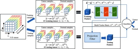
Feature extraction using Tucker tensor decomposition.

3.4. Classification

In this study, 12 hypercubes from 12 mice with head and neck cancers are scanned and used for the hyperspectral image analysis. We choose SVM as the classifier and the Gaussian radial basis function as the kernel function.³⁷ Nested cross validations (CVs) are used to perform model selection and evaluation. We perform leave-one-out outer CV, and threefold inner CV. A grid search is performed in the inner CV on the training data to select the optimal values for parameter C and g over the range of ${\log }_{2}C=\{0;-\mathrm{1,0},\cdots ,4\}$; and ${\log }_{2}g=\{-\mathrm{1,0},\cdots ,4\}$;. Then, a new SVM model is trained with the optimal parameters on 11 mouse data, and the performance of that model is tested on the rest of the mice.

3.5. Postprocessing

After obtaining the probability maps of each tumor image, we proceed to use active contours^38,39 to refine the classification results. Chan-Vese active contour⁴⁰ is a region-based segmentation method which can be used to segment vector-valued images such as RGB images. Standard $L2$ norm is used to compare the image intensity with the mean intensity of the region inside and outside the curve. If the image contains some artifacts, $L2$ norm may not work well. Therefore, we modified the Chan-Vese active contour with $L1$ norm, which compares the image intensity with the median intensity of the region inside and outside the curve. This modification makes the active contour more robust to noises. In this section, we will first introduce the mathematic formulation of the modified $L1$ norm active contour methods.

The energy function with $L1$ norm is defined as follows

$$E(u,v,\mathrm{C})=\int {\int }_{\mathrm{\Omega }}\frac{1}{N}\sum _{i=1}^N|I_i-u_i|\mathrm{d}x\mathrm{d}y+\int {\int }_{\mathrm{\Omega }}\frac{1}{N}\sum _{i=1}^N|I_i-v_i|\mathrm{d}x\mathrm{d}y+\lambda {\int }_C\mathrm{d}s,$$ (5)

where C stands for the curve, $\mathrm{\Omega }$ stands for the area inside C, and ${\mathrm{\Omega }}^c$ stands for the area outside C. The last term penalizes the “shape” of the curve to avoid complicated curves. $N$ is the total number of image bands.

Given the curve C, we want to find the optimal values of $u_i$, $v_i$. By setting $[\delta E(u,v,\mathrm{c})/\delta u_i]=0$ and $[\delta E(u,v,\mathrm{c})/\delta v_i]=0$, we obtain

$$\begin{gathered} \frac{\delta E(u,v,\mathrm{c})}{\delta u_i}=\frac{\delta }{\delta u_i}\int {\int }_{\mathrm{\Omega }}\frac{1}{N}\sum _{i=1}^N|I_i-u_i|\mathrm{d}x\mathrm{d}y \\ =\frac{\delta }{\delta u_i}\int {\int }_{\mathrm{\Omega }}\frac{1}{N}\sum _{i=1}^N\sqrt[2]{{(I_i-u_i)}^2}\mathrm{d}x\mathrm{d}y\frac{I-u_i}{|I-u_i|}=-\frac{1}{N}\int {\int }_{\mathrm{\Omega }}\frac{I_i-u_i}{|I_i-u_i|}\mathrm{d}x\mathrm{d}y=0 \\ \Rightarrow \int {\int }_{\mathrm{\Omega }}\frac{I_i-u_i}{|I_i-u_i|}\mathrm{d}x\mathrm{d}y=0. \end{gathered}$$ (6)

As we know that $I-u_i/|I-u_i|$ is either 1 or $-1$, to make the integration of $1-u_i/|1-u_i|$ inside the curve 0, half of the values should be 1 and the other half of the values should be $-1$; therefore, the optimal value for $u_i$ is the median intensity of the $i$’th image band inside the curve C. Similarly, we know that the optimal value for $v_i$ is the median intensity of the $i$’th image band outside the curve C.

It is expected that the modified active contour with $L1$ norm applied on the RGB probability maps of tumors will further boost the classification performance.

3.6. Comparison with the Spectral-Based Classification Method

To compare the proposed spectral-spatial classification method with the spectral-based method for classifying cancerous and normal tissues, we implement the traditional pixel-wise spectral method as illustrated in Fig. 2(a).

3.6.1. Pixel-wise spectral-based method

If no dimension reduction technique is used, then the normalized reflectance spectra of each pixel with 224 dimensions are directly used as the spectral feature. This method is time consuming due to high-feature dimensions.

3.6.2. PCA-based spectral method

Considering the high dimensions (over 200) of reflectance spectra, PCA is usually applied to reduce the dimensionality. First, the hypercube $(x\times y\times \lambda )$ is rearranged into a 2-D spectral matrix of dimension $M\times \lambda$, where $M=x\times y$ is the total number of pixels, and $\lambda$ is the total number of wavelengths used. So, each row represents the reflectance values from all the bands at one pixel. Then the matrix is centered by subtracting the mean values of each column. Afterward, PCA was performed to calculate the eigenvalues and eigenvectors. Finally, the original hypercube was approximated by the inverse principle component transformation, with the first few bands containing the majority of the variation residing in the original hypercube.⁴¹

3.7. Performance Evaluation Metrics

Accuracy, sensitivity and specificity are commonly used performance metrics for a binary classification task.^42,43 In this study, accuracy is calculated as a ratio of the number of correctly labeled pixels to the total number of pixels in a test image. Sensitivity measures the proportion of actual cancerous pixels (positives) which are correctly identified as such in a test image, whereas specificity measures the proportion of healthy pixels (negatives) which are correctly classified as such in a test image. $F$-score is the harmonic mean of precision (the proportion of correct true positives to all predicted positives) and sensitivity. Table 1 shows the confusion matrix, which contains information about actual and predicted classification results performed by a classifier.

Table 1.

Confusion matrix.

		Predicted results
		Negative (healthy)	Positive (cancerous)
Gold Standard	Negative (healthy)	True negative (TN)	False positive (FP)
	Positive (cancerous)	False negative (FN)	True positive (TP)

The definitions of accuracy, precision, sensitivity, specificity, and $F$-score are defined below:

$$\text{Accuracy}=\frac{\mathrm{TP}+\mathrm{TN}}{\mathrm{TP}+\mathrm{FP}+\mathrm{FN}+\mathrm{TN}};\text{Sensitivity}=\frac{\mathrm{TP}}{\mathrm{TP}+\mathrm{FN}};\text{Specificity}=\frac{\mathrm{TN}}{\mathrm{TN}+\mathrm{FP}}$$

$$\text{Precision}=\frac{\mathrm{TP}}{\mathrm{TP}+\mathrm{FP}};F=2\times \frac{P\text{recision}\times S\text{ensitivity}}{P\text{recision}+S\text{ensitivity}}\mathrm{.}$$

4. Results

To evaluate the proposed tumor detection algorithm, we scanned 12 GFP tumor-bearing mice approximately 2 weeks post-tumor cell injection and distinguished between cancerous and normal tissues based on their spectral differences in this study.

4.1. Data Normalization

To visualize the spectral variation arising from tumor curvature, a region of interest covering the tumor of a mouse was selected on the reflectance composite RGB color image [shown in Figs. 6(a) and 6(d)], and the average spectra for a selection of regions at various locations [denoted by squares in Figs. 6(a) and 6(d)], were obtained by averaging pixel spectra from a square area of $10\times 10\text{\hspace{0.17em}\hspace{0.17em}pixels}$ pixels from those regions. It is obvious that the curvature of the tumor surface causes a scaling difference in the spectra: the spectrum from the center of the tumor exhibited higher reflectance intensity than the spectra from the sides of the tumor and the surrounding normal tissue. This is mainly caused by the relative difference in the path length from different points of the curved tumor surface to the detector. So, it is desirable to minimize the spectral variability caused by tumor curvature.

Fig. 6.

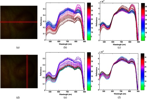
Effects of the pre-processing on spectra as selected from different regions of a mouse image. (a) and (d) are the same region of interest (ROI) covering the tumor area; the horizontal and vertical locations are composed of square areas of $10\times 10\text{\hspace{0.17em}\hspace{0.17em}pixels}$. (b) and (c) show the average spectra of each square from left to right before and after preprocessing. (e) and (f) show the average spectra of each square from top to bottom before and after preprocessing.

Figures 6(b) and 6(e) show the spectral variation along the horizontal direction and vertical direction, respectively. Figures 6(c) and 6(f) show the spectral curve of pixels along the horizontal and vertical directions after data normalization. The color bar varying from green to black in Figs. 6(b) and 6(c) represents the location from left to right, whereas the color bar in (e) and (f) denotes the location from top to bottom. It can be seen that the spectral variance is greatly reduced and the spectral curve is smoothed after applying the preprocessing procedure described in Sec. 3.1. It is reasonable to assume that after preprocessing, the spectral variance arises from the actual difference between normal and cancerous tissues.

4.2. Vascularity Visualization

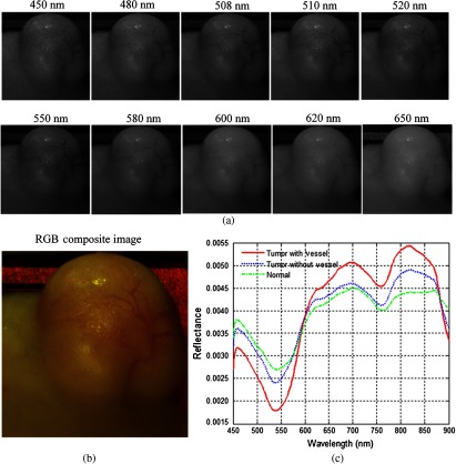
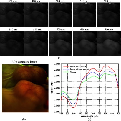
In this study, we acquired hyperspectral reflectance images from both tumors without GFP and tumors with GFP. Figures 7 and 8 show the in vivo hyperspectral reflectance images of a tumor without GFP and a tumor with GFP, respectively.

Fig. 7.

In vivo hyperspectral reflectance imaging of a tumor without GFP. (a) Reflectance images at different wavelength bands. (b) An RGB composite image generated from the tumor hypercube. (c) Red solid line: the average reflectance spectra of the vessels inside tumor region; blue dotted line: the average reflectance spectra of randomly selected nonvessel tumor regions; green dash-dot line: the average of randomly selected normal regions around the tumor.

Fig. 8.

In vivo hyperspectral reflectance imaging of a tumor with GFP. A mirror is used to aid in capturing the entire tumor during imaging. (a) Reflectance images at different wavelength bands. 508 nm and 510 nm are the emission peaks for GFP under blue excitation. (b) An RGB composite image generated from the tumor hypercube. (c) Red solid line: the average reflectance spectra of the vessels inside tumor region; blue dotted line: the average reflectance spectra of randomly selected nonvessel tumor regions; green dash-dot line: the average of randomly selected normal regions around tumors. (Note: pixels are only selected from the tumor region that is not in the mirror).

To visualize the hyperspectral dataset, RGB composite images were generated as shown in Figs. 7(b) and 8(b), and the individual image bands at different wavelengths are shown in Figs. 7(a) and Fig. 8(a). In both cases, vascularity patterns can be clearly visualized at different wavelengths. The skin of nude mice, which covered the tumor, is less than 1-mm thick, so we can visualize tumor vessels through the intact skin even at 450-nm wavelength. It can be seen that the vascular structure became obscured at higher wavelengths, which indicates that light at lower wavelengths is more sensitive to superficial information of tissue and that light at higher wavelengths carries information from deeper tissue due to deeper penetration into tissue.

Wavelengths of 508 and 510 nm are emission peaks of GFP under blue excitation, and image bands at these two wavelengths for both GFP-tumor and non-GFP-tumor were shown in Figs. 7(a) and 8(a). It is worth noting that images obtained at GFP bands did not show higher contrast compared to images at other wavelength bands under white excitation. Therefore, it makes sense to assume that the spectral contrast between cancerous and healthy tissues is not caused by the GFP signals.

Figures 7(c) and 8(c) show the average reflectance spectra of vessels inside tumor regions with a red solid line, the average reflectance spectra of nonvessel tumor regions with the blue dotted line, and the average of randomly selected normal regions around tumors with the green dash-dot line. The reflectance spectra of both tumors show a dip at around 540 to 580 nm, which coincides with hemoglobin’s absorption peaks. Vessel spectra in tumor region $<600\mathrm{nm}$ and $>870\mathrm{nm}$ exhibit lower reflectance than non-vessel tissue, which is consistent with the higher amount of hemoglobin in vessels. In addition, the reflectance spectra of the tumor region is lower than that of the normal region $<600\mathrm{nm}$ and $>870\mathrm{nm}$, which also indicates that tumors have a higher amount of hemoglobin compared to normal tissue.

4.3. Spectra Analysis

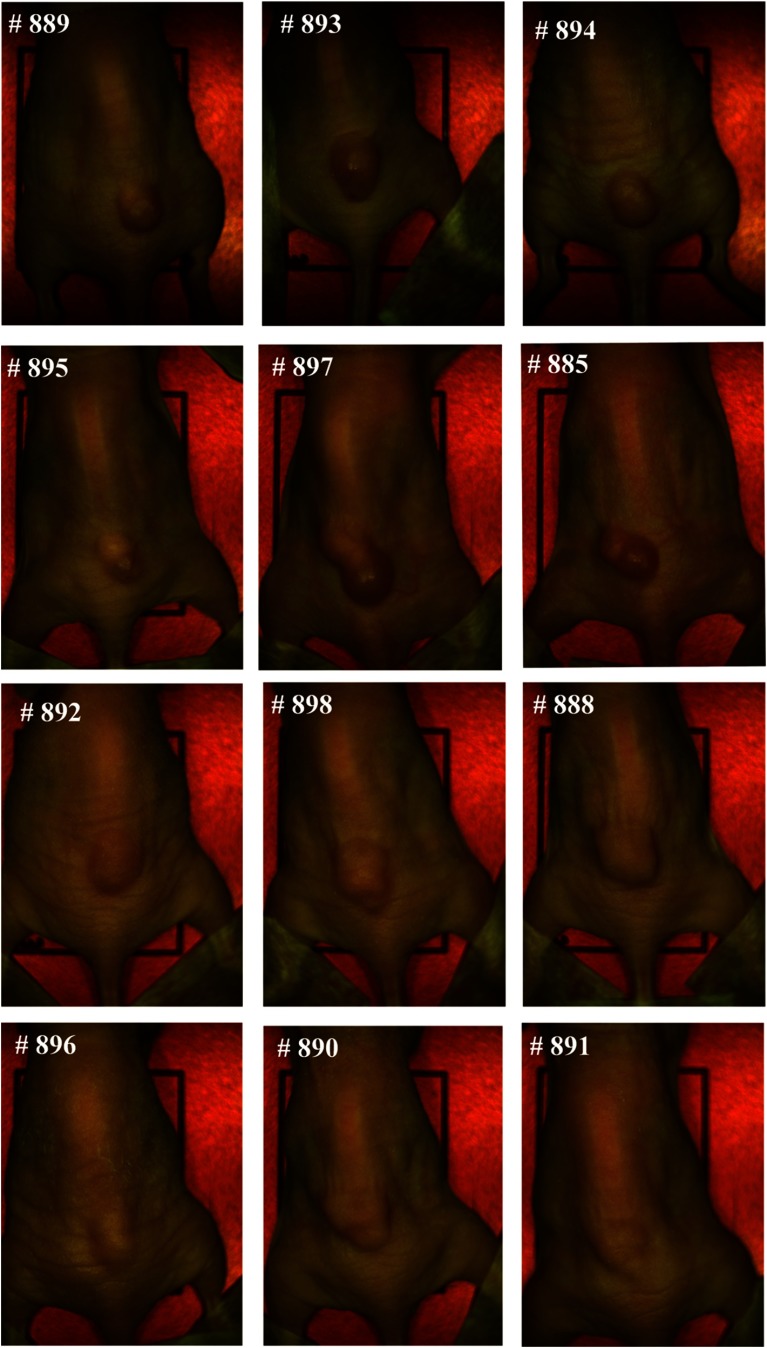
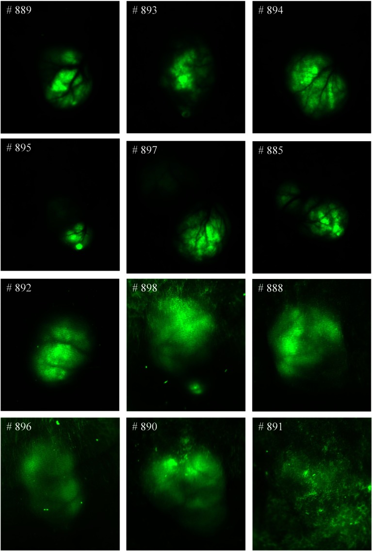
Figure 9 shows the RGB composite images of hyperspectral reflectance images for all 12 mice used for the evaluation of the spectral-spatial classification method. The numbers on the left corners of the mouse images denote the ID on the ear tags of the mice; hence, they are used to help identify different mice. As can be seen, tumor volumes varied from $92{\mathrm{mm}}^3$ to about $200{\mathrm{mm}}^3$ at the time of imaging. Figure 10 shows the RGB composite images of hyperspectral fluorescence images for tumors with GFP. In both reflectance and fluorescence images, vascular patterns can also be visualized in some tumors, such as # 885, # 889, etc. Fluorescence images showed vascular beds more clearly; the tumor regions were lighted as green due to GFP emission peaks at 508 and 510 nm.

Fig. 9.

RGB composite images of the reflectance hyperspectral images of the 12 mice used for the evaluation of the spectral-spatial algorithm. The number on the top left corner of each image represents the ID on the ear tag of a mouse.

Fig. 10.

RGB composite images of hyperspectral fluorescence images for the tumors with green fluorescence protein (GFP). Tumors show GFP signals on the images.

Although the current gold standard for cancer diagnosis remains histological assessment of hematoxylin and eosin stained tissue, the ex vivo tissue specimen undergoes deformations, including shrinkage, tearing, and distortion, which makes it difficult to align the ex vivo gold standard with in vivo tumor tissue. However, the in vivo GFP images provided a much better alignment with hyperspectral reflectance images, since they were acquired in vivo immediately after the acquisition of reflectance images for each mouse, and the tumor and surrounding normal tissue exhibited high contrast in the GFP images. In this study, tumor regions were identified manually on the GFP images, and the classification results were then compared with the manual maps. As shown in Fig. 10, the GFP images for the tumors #888, #898, #896, #890, #891 were not clear due to high tissue autofluorescence caused by the food residuals and other wastes on the skin. For these images, we first performed spectral unmixing using the commercial Maestro software to better separate the tumors and surrounding tissues and then manually segmented the tumors. Since human tissue does not naturally contain GFP, registration methods are desirable to align the in vivo hyperspectral images with ex vivo histological images as discussed in Ref. 14, in order to move forward to future human studies.

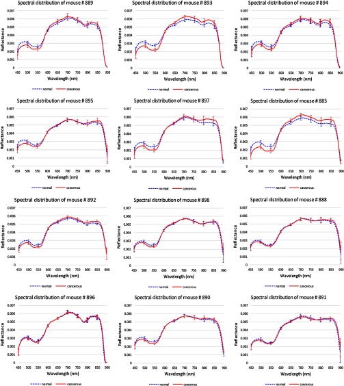
Figure 11 shows the average reflectance spectra and standard deviations of the cancerous tissue regions from 450 to 900 nm in the red solid line, and the average reflectance spectra and standard deviations of the surrounding healthy tissues in the blue dotted line. To make it easier to visualize the two spectra curves, we only showed the standard deviations at the wavelengths from 450 to 900 nm with an increment of 50 nm. Due to tumor heterogeneities in morphology, reflectance spectra at different locations varied from each other and deviated from their average reflectance spectra.

Fig. 11.

Reflectance spectra of 12 mice. Red solid line: the average spectra of cancerous tissues in each mouse. Blue dotted line: the average spectra of healthy surrounding tissues in each mouse. The error bars in both lines represent the standard deviations of spectra within each region.

Hemoglobin characteristics were shown in these reflectance spectra, which could be indicative of cancer formation. It was found that the normalized reflectance intensity of tumor was lower below 600 nm for all these mice and lower above 870 nm for some of the mice such as #894 and #885. This indicated that the amount of hemoglobin was higher in tumors than normal tissues, which may be due to the angiogenesis during tumor formation.

We have demonstrated that the vascularity patterns can be visualized from hyperspectral reflectance imaging (Sec. 4.2), and the amount of hemoglobin and oxygenated hemoglobin also varies between cancerous and healthy tissues. In addition, vascular density in oral cancers has been shown to be an important biomarker for some cancers.⁴⁴ These observations confirm that tissue reflectance spectra measured from 450 to 900 nm provide valuable information for differentiating between tumor and normal tissues. Therefore, hyperspectral reflectance imaging has the potential to detect tumors noninvasively through intact skin.

It was noted that the reflectance spectra differences between tumor and normal tissues were relatively small in mice #888, #898, #896, #890, and #891 compared to the rest of the mice, which coincided with the lower contrast between tumor and surrounding tissue in fluorescence images of these mice. This might be because the reflected light from the tissue was further randomly scattered by the food and wastes adhered to the tissue surface, which obscured the differences between cancerous and healthy tissue caused by the biochemical and morphological changes during neoplastic changes.

4.4. Comparison with Spectral Method

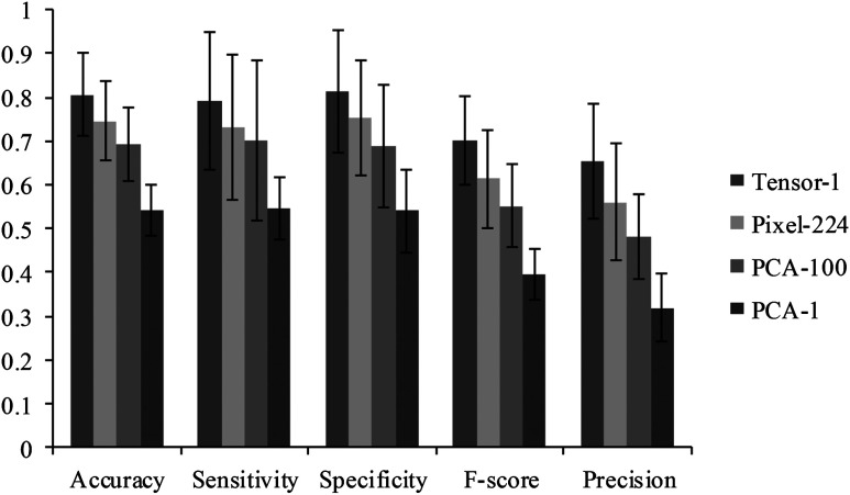
To compare the spectral spatial classification method with the spectral classification method, we implemented three spectral methods as shown in Fig. 12. “Tensor-1” denoted the spectral spatial classification method which represents each pixel with a one-dimensional (1-D) tensor feature. “Pixel-224” denoted the pixel-wise method which represents each pixel with a vector consisting of 224 reflectance values. “PCA-100” utilized PCA to reduce the pixel-wise feature dimension from 224 to the top 100 most significant features. “PCA-1” utilized PCA to reduce the pixel-wise feature dimension from 224 to the top most significant feature which represents the most variances. For all four methods, a KNN classifier is employed to classify the data with leave-one-out CV. Figure 12 compared the average and standard deviation of accuracy, sensitivity, specificity, $F$-score, and precision of the 12 mice for all four methods.

Fig. 12.

The performance of the Tensor-1, PAC-1, PAC-100, Pixel-224 classification methods. See the text for the definitions of the four methods.

As can be seen from Fig. 12, the spectral spatial method with a 1-D tensor feature outperformed the rest of the spectral-based methods. Although the first PCA image band explained about 85% of the variance in the feature vector, the classification accuracy of the PCA-1 method only achieved 54%. More than 100 features were required in order to obtain an accuracy of $>69\%$ with the PCA dimension reduction method, while the top tensor feature alone achieved an accuracy of 80%, which exhibited a strong discriminatory ability for differentiating tumors from normal tissue. It was found that the feature dimension and classification time were significantly reduced without sacrificing the accuracy with the tensor-based spectral spatial method, while higher feature dimensions and longer classification times were needed in order to achieve comparable accuracy with the PCA-based spectral method.

4.5. Classification Results of the Spectral-Spatial Method

The spectral-spatial classification algorithm was implemented in MATLAB (Version R2013a, Mathworks, Natick, Massachusetts) using a high-performance computer with 128 GB RAM and 32 CPUs of 3.1 GHz. The region of interest (ROI) selected in each mouse image was of the dimension $435\times 390$. So, each testing image ROI consisted of 168,004 pixels. Since surrounding tissue areas in the selected ROI were generally larger than the tumor region, the same number of healthy tissue pixels as the number of tumor pixels was randomly chosen from the surrounding tissue to build a balanced training dataset.

After completion of the SVM training process with optimal parameters, it usually takes about 2 min to test the hypercube image data of one mouse. The computation performance can be improved by implementing the algorithm in parallel computing and by using C++ language.

Figures 13–16 show the SVM probability maps of all 12 tumor hypercubes in the first row and the refined classification results by active contour in the second row. As can be seen from these figures, SVM probability maps exhibited salt and pepper appearances, while active contour reduced both the false positives and false negatives in the normal tissue regions.

Fig. 13.

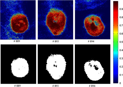
Classification maps. The first row represents the SVM probability map for Mice # 889, # 893, # 894, and the color bar on the right denotes the probability with different colors. The second row represents the corresponding binary tumor maps after active contour postprocessing.

Fig. 14.

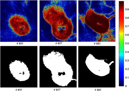
Classification maps. The first row represents the SVM probability map for Mice # 895, # 897, # 885, and the color bar on the right denotes the probability with different colors. The second row represents the corresponding binary tumor maps after active contour postprocessing.

Fig. 15.

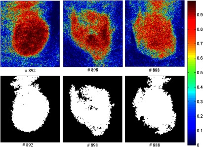
Classification maps. The first row represents the SVM probability map for Mice # 892, # 898, # 888, and the color bar on the right denotes the probability with different colors. The second row represents the corresponding binary tumor maps after active contour postprocessing.

Fig. 16.

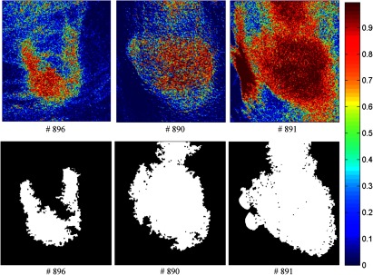
Classification maps. The first row represents the SVM probability map for Mice # 896, # 890, # 891, and the color bar on the right denotes the probability with different colors. The second row represents the corresponding binary tumor maps after active contour postprocessing.

Mice #889, #893, and #894 in Fig. 13 and Mouse #895 in Fig. 14 were well classified with an average accuracy, sensitivity, and specificity of 96.1%, 93.2%, and 97.5%, respectively. Mouse # 897 and Mouse # 885 in Fig. 14 exhibited misclassification in the blood vessels within normal tissue region (as shown in the RGB images in Fig. 9). The binary classification only sorts the pixels into two categories: tumor or normal tissue. Blood vessels showed strong hemoglobin signals, which might appear closer to the tumor regions, therefore, were misclassified as tumor pixels.

Mice # 892, # 898, and # 888 in Fig. 15 contained false positives in the normal tissue which was curved and highly resembled the tumor tissue. Mice # 896, # 890, and # 891 in Fig. 16 were not classified satisfactory, which was consistent with the observations from the GFP images in Fig. 11. Due to the random scattering caused by the tissue artifacts, the reflectance spectral differences between cancerous and normal tissues were obscured. Therefore, the classification algorithm was not able to achieve satisfactory results.

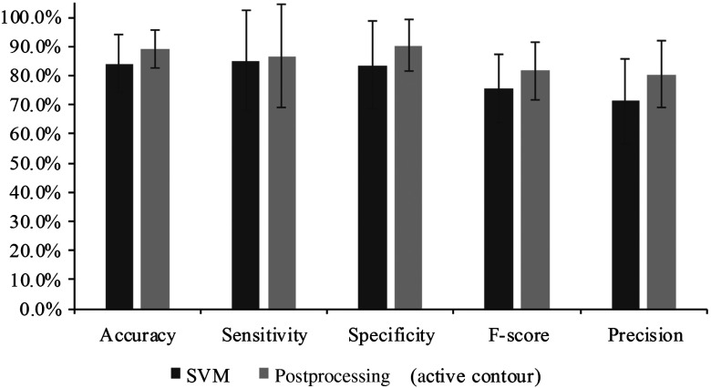
Figure 17 shows the comparison of the classification performance before postprocessing and after the processing. The average accuracy, sensitivity, specificity, $F\_\mathrm{score}$, and precision of all 12 mice with standard deviations as error bars were plotted. The active contour postprocessing procedure further improved the average accuracy, sensitivity, and specificity of the 12 mice by 5.1%, 1.6%, and 6.7%, respectively.

Fig. 17.

Comparison between the classification results before and after postprocessing. As can be seen, the active contour post-processing method improved the classification performance of SVM in all the metrics.

The classification performances of all mice after postprocessing were listed in Table 2. The average accuracy, sensitivity, and specificity of 12 mice were 89.1%, 86.8%, and 90.4%, respectively. Based on the above analysis, we knew that the bad performance of the last three mice (#896, #890, #891) shown in Table 2 were caused by the tissue artifacts. If we remove these three mice, the average accuracy, sensitivity, and specificity were 91.9%, 93.7%, and 91.3%, respectively.

Table 2.

Summary of the classification performance.

Mice ID	Accuracy (%)	Sensitivity (%)	Specificity (%)
# 889	97.1	94.9	97.7
# 893	96.9	96.0	97.3
# 894	95.8	88.7	97.7
# 895	94.5	96.3	94.2
# 897	91.4	91.3	91.5
# 885	90.9	99.8	88.6
# 892	85.0	99.9	80.0
# 898	88.3	92.4	86.6
# 888	86.8	84.2	88.4
# 896	85.2	55.0	96.2
# 890	79.1	46.2	97.9
# 891	78.4	96.7	68.3
Mean	89.1	86.8	90.4
Std	6.5	17.6	8.9

5. Discussion

This paper has described and evaluated a spectral-spatial classification method for distinguishing cancerous and healthy tissue in vivo in a head and neck cancer animal model and demonstrated that HSI combined with a spectral-spatial classification method holds great promise for noninvasive diagnosis of cancer.

The basis for cancer detection using HSI and spectral-spatial method arises from the differences in the spectra obtained from the normal and diseased tissue due to the multiple physiological changes associated with tissue transformation from healthy to cancerous stages. During disease progression, healthy tissue transforms to pathological tissue with biochemical and morphological changes, such as increase in epithelial thickness, nuclear size, nuclear to cytoplasmic ratio, changes in the chromatin texture and collagen content, and angiogenesis.⁴⁵ These changes modify the diffusely reflected light, therefore, reflectance spectra exhibit spectral features associated with different biochemical and morphological characteristics of cancerous and normal tissues.

The motivation for developing spectral-spatial classification algorithms is that HSI is limited by the user’s ability to pull relevant information out of the enormous amount of data, and the development of advanced data mining methods utilizing the abundant spectral and spatial information contained in hypercube is desirable for classification of lesions and healthy tissue. As preclinical and clinical research with HSI moves forward, more and more datasets are going to be acquired and stored. On the one hand, spectral databases for different types of pathological tissues, cells, and molecules could aid in a better interpretation of hyperspectral images. On the other hand, the hidden patterns, unknown correlations, and useful diagnostic information could be uncovered and fully utilized with the help of machine learning and data mining methods. For example, classification models build upon large datasets would provide a valuable tool for quantitative diagnosis of cancer.

The prominent advantage of HSI is that it combines the wide-field imaging with spectroscopy. Additionally, HSI is a noninvasive, nonionizing imaging technology, which does not require contrast agents. Hyperspectral images have more spectral channels and higher spectral resolution than RGB images, which might carry more useful information for characterization of physiology and pathophysiology. Spectroscopy measures tissue point by point, which might miss the most malignant potential. HSI captures the spectral images of a large area of tissue, which overcomes the under-sampling problem associated with spectroscopy and biopsy.

The application of HSI can be limited because it examines only the areas of tissue near the surface, which could be a big problem for imaging deep resided tumors inside tissue in vivo. The optical penetration depth is defined as the tissue thickness that reduces the light intensity to 37% of the intensity at the surface. Bashkatov et al.⁴⁶ measured the optical penetration depth of light into skin over the wavelength range from 400 to 2000 nm. It was observed that light penetration depth at a wavelength of 450 nm was about 0.5 mm, and light at $>500\mathrm{nm}$ had a penetration depth of above 1 mm. The maximum penetration depth was found to be 3.5 mm at wavelength 1090 nm. Given that the skin of the nude mice in our experiment was $<1\mathrm{mm}$ and that the reflectance images starting from 450 nm already showed the vascular beds of the tumor, it makes sense to assume that the reflectance spectra acquired from 450 to 900 nm carries diagnostic information about tumors underneath the skin. Therefore, hyperspectral reflectance imaging combined with a spectral-spatial classification method scan distinguishes between tumors and surrounding tissue through intact skins.

To further extend the application of the proposed technique, we plan to explore the ability of HSI at the near-infrared region $>900\mathrm{nm}$ for noninvasive cancer detection in the future, because near-infrared light has a relatively deep tissue penetration compared to visible light. Since the near-infrared spectra are complicated by the presence of overlapping water bands, and vibrational overtones, it becomes more difficult to interpret the large volume of hyperspectral dataset by decomposing it into different tissue components. Therefore, spectral-spatial classification based on the spectral differences of cancerous and healthy tissue pixels would be of great importance for statistical analysis of hypercubes.

The computational requirement for handling a vast amount of hyperspectral dataset is demanding in terms of the computer resources and time costs. Motion artifacts may also deteriorate the image quality due to longer data acquisition times for large datasets. Therefore, optimal band selection will be performed before applying the spectral-spatial classification method in our future research. Once the reflectance spectral bands which best characterize the tissue physiology are selected, only spectral images at specific wavelengths will be acquired and used for further analysis.

As an emerging imaging technology in medicine, HSI can have many potential applications, not only for cancer detection but also for other medical applications such as image-guided surgery. Studies of HSI for cancer diagnosis have been investigated in the cervix, breast, skin, oral cavity, esophageal, colon, kidney, bladder, etc. HSI has also been explored for surgical guidance in mastectomy, gall bladder surgery, cholecystectomy, nephrectomy, renal surgery, abdominal surgery, etc. A detailed review for applications of medical HSI can be found in Ref. 6. Recent studies also employed HSI for monitoring of chemotherapy on cancers.⁴⁷

6. Conclusion

In this study, we described and validated a spectral-spatial classification framework based on tensor modeling for HSI in the application of head and neck cancer detection. This method characterized both spatial and spectral properties of the hypercube and effectively performed dimensionality reduction. In an animal head and neck cancer model, the proposed classification method was able to distinguish between tumor and normal tissues with an average sensitivity and specificity of 93.7%, and 91.3%, respectively. The results from this study demonstrated that the combination of HSI with spectral-spatial classification methods may enable accurate and quantitative detection of cancers in a noninvasive manner.

Biographies

Guolan Lu is a PhD student in the Department of Biomedical Engineering at Emory University and Georgia Institute of Technology, Atlanta, Georgia.

Baowei Fei is associate professor in the Department of Radiology and Imaging Sciences at Emory University and in the Department of Biomedical Engineering at Emory University and Georgia Institute of Technology. He is a Georgia Cancer Coalition Distinguished Scholar and director of the Quantitative BioImaging Laboratory (www.feilab.org) at Emory University School of Medicine.

Biographies of the other authors are not available.

References

- 1.Siegel R., et al. , “Cancer statistics,” Cancer J. Clin. 64(1), 9–29 (2014). 10.3322/caac.21208 [DOI] [PubMed] [Google Scholar]
- 2.Gerstner A. O., “Early detection in head and neck cancer–current state and future perspectives,” GMS Curr. Top. Otorhinolaryngol. Head Neck Surg. 7(Doc06), 1–24 (2008). [PMC free article] [PubMed] [Google Scholar]
- 3.van den Brekel M. W. M., et al. , “Observer variation in the histopathologic assessment of extranodal tumor spread in lymph node metastases in the neck,” Head Neck 34(6), 840–845 (2012). 10.1002/hed.v34.6 [DOI] [PubMed] [Google Scholar]
- 4.Roblyer D., et al. , “Multispectral optical imaging device for in vivo detection of oral neoplasia,” J. Biomed. Opt. 13(2), 024019 (2008). 10.1117/1.2904658 [DOI] [PMC free article] [PubMed] [Google Scholar]
- 5.Ismail S. M., et al. , “Observer variation in histopathological diagnosis and grading of cervical intraepithelial neoplasia,” Br. Med. J. 298(6675), 707–710 (1989). 10.1136/bmj.298.6675.707 [DOI] [PMC free article] [PubMed] [Google Scholar]
- 6.Lu G., Fei B., “Medical hyperspectral imaging: a review,” J. Biomed. Opt. 19(1), 010901 (2014). 10.1117/1.JBO.19.1.010901 [DOI] [PMC free article] [PubMed] [Google Scholar]
- 7.Zuzak K. J., et al. , “Visible and infrared hyperspectral visualization of normal and ischemic tissue,” in Engineering in Medicine and Biology, 1999. 21st Annual Conference and the 1999 Annual Fall Meeting of the Biomedical Engineering Society, BMES/EMBS Conference, 1999, Proceedings of the First Joint, Atlanta, GA, p. 1118 (1999). [Google Scholar]
- 8.Akbari H., et al. , “Detection and analysis of the intestinal ischemia using visible and invisible hyperspectral imaging,” IEEE Trans. Biomed. Eng. 57(8), 2011–2017 (2010). 10.1109/TBME.2010.2049110 [DOI] [PubMed] [Google Scholar]
- 9.Chin M. S., et al. , “Hyperspectral imaging for early detection of oxygenation and perfusion changes in irradiated skin,” J. Biomed. Opt. 17(2), 026010 (2012). 10.1117/1.JBO.17.2.026010 [DOI] [PubMed] [Google Scholar]
- 10.Akbari H., et al. , “Hyperspectral imaging and quantitative analysis for prostate cancer detection,” J. Biomed. Opt. 17(7), 076005 (2012). 10.1117/1.JBO.17.7.076005 [DOI] [PMC free article] [PubMed] [Google Scholar]
- 11.Akbari H., et al. , “Cancer detection using infrared hyperspectral imaging,” Cancer Sci. 102(4), 852–857 (2011). 10.1111/cas.2011.102.issue-4 [DOI] [PMC free article] [PubMed] [Google Scholar]
- 12.Lu G., et al. , “Spectral-spatial classification using tensor modeling for cancer detection with hyperspectral imaging,” Proc. SPIE 9034, 903413 (2014). 10.1117/12.2043796 [DOI] [PMC free article] [PubMed] [Google Scholar]
- 13.Pike R., et al. , “A minimum spanning forest based hyperspectral image classification method for cancerous tissue detection,” Proc. SPIE 9034, 90341W (2014). 10.1117/12.2043848 [DOI] [PMC free article] [PubMed] [Google Scholar]
- 14.Lu G., et al. , “Hyperspectral imaging for cancer surgical margin delineation: registration of hyperspectral and histological images,” Proc. SPIE 9036, 90360S (2014). 10.1117/12.2043805 [DOI] [PMC free article] [PubMed] [Google Scholar]
- 15.Liu Z., Wang H. J., Li Q. L., “Tongue tumor detection in medical hyperspectral images,” Sensors 12(1), 162–174 (2012). 10.3390/s120100162 [DOI] [PMC free article] [PubMed] [Google Scholar]
- 16.Masood K., Rajpoot N., “Texture based classification of hyperspectral colon biopsy samples using CLBP,” in IEEE Int. Symposium on Biomedical Imaging: From Nano to Macro, 2009. ISBI '09, Boston, Massachusetts, pp. 1011–1014 (2009). [Google Scholar]
- 17.Masood K., Rajpoot N., “Spatial analysis for colon biopsy classification from hyperspectral imagery,” Ann. BMVA 2008(4), 1–16 (2008). [Google Scholar]
- 18.Masood K., “Hyperspectral imaging with wavelet transform for classification of colon tissue biopsy samples,” Proc. SPIE 7073, 707319 (2008). 10.1117/12.797667 [DOI] [Google Scholar]
- 19.Qin X., et al. , “Automatic segmentation of right ventricle on ultrasound images using sparse matrix transform and level set,” Proc. SPIE 8669, 86690Q (2013). 10.1117/12.2006490 [DOI] [PMC free article] [PubMed] [Google Scholar]
- 20.Qin X., Cong Z., Fei B., “Automatic segmentation of right ventricular ultrasound images using sparse matrix transform and a level set,” Phys. Med. Biol. 58(21), 7609 (2013). 10.1088/0031-9155/58/21/7609 [DOI] [PMC free article] [PubMed] [Google Scholar]
- 21.Renard N., Bourennane S., “Improvement of target detection methods by multiway filtering,” IEEE Trans. Geosci. Remote Sens. 46(8), 2407–2417 (2008). 10.1109/TGRS.2008.918419 [DOI] [Google Scholar]
- 22.Lin T., Bourennane S., “Hyperspectral image processing by jointly filtering wavelet component tensor,” IEEE Trans. Geosci. Remote Sens. 51(6), 3529–3541 (2013). 10.1109/TGRS.2012.2225065 [DOI] [Google Scholar]
- 23.Renard N., Bourennane S., Blanc-Talon J., “Denoising and dimensionality reduction using multilinear tools for hyperspectral images,” IEEE Trans. Geosci. Remote Sens. Lett. 5(2), 138–142 (2008). 10.1109/LGRS.2008.915736 [DOI] [Google Scholar]
- 24.Renard N., Bourennane S., “Dimensionality reduction based on tensor modeling for classification methods,” IEEE Trans. Geosci. Remote Sens. 47(4), 1123–1131 (2009). 10.1109/TGRS.2008.2008903 [DOI] [Google Scholar]
- 25.Bourennane S., Fossati C., Cailly A., “Improvement of classification for hyperspectral images based on tensor modeling,” IEEE Trans. Geosci. Remote Sens. Lett. 7(4), 801–805 (2010). 10.1109/LGRS.2010.2048696 [DOI] [Google Scholar]
- 26.Liangpei Z., et al. , “Tensor discriminative locality alignment for hyperspectral image spectral-spatial feature extraction,” IEEE Trans. Geosci. Remote Sens. 51(1), 242–256 (2013). 10.1109/TGRS.2012.2197860 [DOI] [Google Scholar]
- 27.Hemissi S., et al. , “Multi-spectro-temporal analysis of hyperspectral imagery based on 3-D spectral modeling and multilinear algebra,” IEEE Trans. Geosci. Remote Sens. 51(1), 199–216 (2013). 10.1109/TGRS.2012.2200486 [DOI] [Google Scholar]
- 28.Velasco-Forero S., Angulo J., “Classification of hyperspectral images by tensor modeling and additive morphological decomposition,” Pattern Recognit. 46(2), 566–577 (2013). 10.1016/j.patcog.2012.08.011 [DOI] [Google Scholar]
- 29.Phan A. H., Cichocki A., “Tensor decompositions for feature extraction and classification of high dimensional datasets,” Nonlinear Theory and Its Applications, IEICE 1(1), 37–68 (2010). [Google Scholar]
- 30.Zhang X., et al. , “Understanding metastatic SCCHN cells from unique genotypes to phenotypes with the aid of an animal model and DNA microarray analysis,” Clin. Exp. Metastasis 23(3–4), 209–222 (2006). 10.1007/s10585-006-9031-0 [DOI] [PubMed] [Google Scholar]
- 31.Panasyuk S. V., et al. , “Medical hyperspectral imaging to facilitate residual tumor identification during surgery,” Cancer Biol. Ther. 6(3), 439–446 (2007). 10.4161/cbt [DOI] [PubMed] [Google Scholar]
- 32.Claridge E., Hidovic-Rowe D., “Model based inversion for deriving maps of histological parameters characteristic of cancer from ex-vivo multispectral images of the colon,” IEEE Trans Med Imaging 33(4), 822–835 (2014). 10.1109/TMI.2013.2290697 [DOI] [PubMed] [Google Scholar]
- 33.Qin X., Fei B., “Measuring myofiber orientations from high-frequency ultrasound images using multiscale decompositions,” Phys. Med. Biol. 59(14), 3907–3924 (2014). 10.1088/0031-9155/59/14/3907 [DOI] [PMC free article] [PubMed] [Google Scholar]
- 34.Qin X., et al. , “Extracting Cardiac Myofiber Orientations from High Frequency Ultrasound Images,” Proc. SPIE 8675, 867507 (2013). 10.1117/12.2006494 [DOI] [PMC free article] [PubMed] [Google Scholar]
- 35.Kolda T. G., Bader B. W., “Tensor decompositions and applications,” SIAM Rev. 51(3), 455–500 (2009). 10.1137/07070111X [DOI] [Google Scholar]
- 36.Cichocki A., “Tensor decompositions: a new concept in brain data analysis?,” J. SICE Control Meas. Syst. Integr. 50(7), 507–517 (2011). [Google Scholar]
- 37.Chang C.-C., Lin C.-J., “LIBSVM: a library for support vector machines,” ACM Trans. Intell. Syst. Technol. 2(3), 27 (2011). 10.1145/1961189 [DOI] [Google Scholar]
- 38.Kass M., Witkin A., Terzopoulos D., “Snakes: active contour models,” Int. J. Comput. Vision 1(4), 321–331 (1988). 10.1007/BF00133570 [DOI] [Google Scholar]
- 39.Qin X., Wang S., Wan M., “Improving reliability and accuracy of vibration parameters of vocal folds based on high-speed video and electroglottography,” IEEE Trans. Biomed. Eng. 56(6), 1744–1754 (2009). 10.1109/TBME.2009.2015772 [DOI] [PubMed] [Google Scholar]
- 40.Chan T. F., Sandberg B. Y., Vese L. A., “Active contours without edges for vector-valued images,” J. Visual Commun. Image Represent. 11(2), 130–141 (2000). 10.1006/jvci.1999.0442 [DOI] [Google Scholar]
- 41.Rodarmel C., Shan J., “Principal component analysis for hyperspectral image classification,” Survey. Land Inf. Sci. 62(2), 115–122 (2002). [Google Scholar]
- 42.Lv G., Yan G., Wang Z., “Bleeding detection in wireless capsule endoscopy images based on color invariants and spatial pyramids using support vector machines,” in Engineering in Medicine and Biology Society, EMBC, 2011 Annual International Conference of the IEEE, Boston, Massachusetts, pp. 6643–6646 (2011). [DOI] [PubMed] [Google Scholar]
- 43.Qin X., et al. , “Breast tissue classification in digital tomosynthesis images based on global gradient minimization and texture features,” Proc. SPIE 9034, 90341V (2014). 10.1117/12.2043828 [DOI] [PMC free article] [PubMed] [Google Scholar]
- 44.Bedard N., et al. , “Multimodal snapshot spectral imaging for oral cancer diagnostics: a pilot study,” Biomed. Opt. Express 4(6), 938–949 (2013). 10.1364/BOE.4.000938 [DOI] [PMC free article] [PubMed] [Google Scholar]
- 45.Stephen M. M., et al. , “Diagnostic accuracy of diffuse reflectance imaging for early detection of pre-malignant and malignant changes in the oral cavity: a feasibility study,” BMC Cancer 13(1), 1–9 (2013). 10.1186/1471-2407-13-278 [DOI] [PMC free article] [PubMed] [Google Scholar]
- 46.Bashkatov A., et al. , “Optical properties of human skin, subcutaneous and mucous tissues in the wavelength range from 400 to 2000 nm,” J. Phys. 38(15), 2543–2555 (2005). 10.1088/0022-3727/38/15/004 [DOI] [Google Scholar]
- 47.Kainerstorfer J. M., et al. , “Evaluation of non-invasive multispectral imaging as a tool for measuring the effect of systemic therapy in Kaposi sarcoma,” PloS One 8(12), e83887 (2013). 10.1371/journal.pone.0083887 [DOI] [PMC free article] [PubMed] [Google Scholar]