Parent of Origin, Mosaicism, and Recurrence Risk: Probabilistic Modeling Explains the Broken Symmetry of Transmission Genetics

Abstract

Most new mutations are observed to arise in fathers, and increasing paternal age positively correlates with the risk of new variants. Interestingly, new mutations in X-linked recessive disease show elevated familial recurrence rates. In male offspring, these mutations must be inherited from mothers. We previously developed a simulation model to consider parental mosaicism as a source of transmitted mutations. In this paper, we extend and formalize the model to provide analytical results and flexible formulas. The results implicate parent of origin and parental mosaicism as central variables in recurrence risk. Consistent with empirical data, our model predicts that more transmitted mutations arise in fathers and that this tendency increases as fathers age. Notably, the lack of expansion later in the male germline determines relatively lower variance in the proportion of mutants, which decreases with paternal age. Subsequently, observation of a transmitted mutation has less impact on the expected risk for future offspring. Conversely, for the female germline, which arrests after clonal expansion in early development, variance in the mutant proportion is higher, and observation of a transmitted mutation dramatically increases the expected risk of recurrence in another pregnancy. Parental somatic mosaicism considerably elevates risk for both parents. These findings have important implications for genetic counseling and for understanding patterns of recurrence in transmission genetics. We provide a convenient online tool and source code implementing our analytical results. These tools permit varying the underlying parameters that influence recurrence risk and could be useful for analyzing risk in diverse family structures.

Introduction

New mutations are the sole source of disease risk for genetic disorders that eliminate reproductive fitness and for lethal alleles that can only exist in a mosaic state. Likewise, new mutations account for approximately one-third of disease risk in severe X-linked recessive conditions that diminish reproduction. In some instances, these new mutations are mitotic in origin (they arise during embryologic development of a parent) and are present in a low-level mosaic state. Such mutations can include single-nucleotide variations (SNVs), indels, nonrecurrent copy-number variations (CNVs), and other nonrecurrent copy-number-neutral structural variations.¹ Importantly, these mutations can be present in the germline of parents and can be potentially recurrently transmitted to future offspring.^2–4 Unexpected recurrences can occur, as evidenced by multiple affected children harboring the same apparently de novo variation. The birth of a single child with a severe genetic disease presents considerable psychological, social, and economic challenges; consequently, recurrence of the same disorder in a second child is a situation many couples prefer to avoid.⁵ Families who have had children affected by apparently de novo mutations can therefore benefit from well-informed risk counseling to make reproductive choices and plan prenatal care for additional pregnancies. These recurrence-risk estimates are an important aspect of the health care provided to such couples, particularly in severe and highly penetrant genetic disorders for which medical therapy remains limited.

Geneticists commonly use the value of <1% to estimate the risk of recurrence for simplex de novo mutations⁶ to be transmitted to additional pregnancies. However, consideration of the literature shows that this risk assessment is often inconsistent with empirical risk for some specific disorders,⁷ particularly those caused by mutations in genes located on the X chromosome.^8,9 These examples provide insight into understanding exceptions to rarity of recurrence of apparently de novo mutations: males affected by X-linked recessive conditions necessarily harbor mutations on the chromosome inherited from their mothers. This maternal bias stands in contrast to the observations that most new mutations arise in the paternal lineage and that the risk of de novo mutation increases with paternal age.^10,11 This paternal bias is broadly consistent with the mitotic origin of many de novo mutations and the additional mitoses experienced by germ cells as fathers age.

We hypothesized that sexual dimorphism in gametogenesis might underlie the juxtaposition of these contrasting biases in higher recurrence risk for X-linked disease and the increased paternal origin of most de novo transmitted mutations. To address this hypothesis, we developed a comprehensive, flexible mathematical model that describes the emergence of new transmitted variants. We show how recurrence risk can be computed on the basis of conditional probability analyses applied to these models in the context of observed affected offspring. These analyses give a comprehensive picture of the emergence of de novo variation and a systematic framework for quantitative analysis of recurrence. The main conclusion of our work is that the parent of origin and the presence of parental somatic mosaicism are major determinants of recurrence risk.

Material and Methods

Models of Mutation and Germline Development

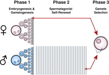
For our investigations, we utilized multitype Galton-Watson processes to model gametogenesis. These approaches are well established in probability theory and have been used for over a century; however, they have seldom been used in statistical genetics. Previous studies of mosaicism led us to hypothesize that this modeling framework could be useful in the analysis of sexual dimorphisms in gametogenesis.⁴ Our model of gametogenesis is composed of three stages (Figure 1). We can optionally include a fourth initial stage that allows stochastic exponential growth without mutation to exclude extremely early embryologic mutations that potentially cause the somatically mosaic parent to be affected. In the first stage of our main model, we consider clonal expansion that results in the initial germ pool during embryogenesis. This expansion phase is parameterized by three variables: the doubling rate of wild-type cells (p), the doubling rate of mutant cells (q), and the per-mitosis mutation rate (λ₁). In the second male-specific stage, we consider the self-renewing process of spermatogenesis. This phase is relatively stable in terms of the total population size and is parameterized by five variables: the doubling rate of wild-type spermatogonial cells (α), the self-renewal rate of wild-type cells (β), the doubling rate of mutant spermatogonial cells (γ), the self-renewal rate of mutant cells (ξ), and the per-mitosis mutation rate (λ₂). The final phase is meiosis, where diploid mutant cells give rise to haploid mutant gametes at a rate of 50% of the pool of mutant cells. We then select a single gamete from each parent to determine transmission.

Figure 1.

Stochastic-Process Model of Sexual Dimorphisms during Gametogenesis

Phase 1: both males and females experience a stochastic exponential cell-expansion phase modeling embryogenesis and germ cell proliferation. Mutations can arise in any cell division, and if they persist in the clonal lineage, they could ultimately be available to be transmitted to the next generation.

Phase 2: in males, expansion is followed by a stochastic but nonexpanding self-renewal process modeling spermatogenesis.

Phase 3: a single sperm and egg are randomly sampled after meiosis to fertilize an offspring. Adapted from Campbell et al.⁴ with permission.

We previously developed exact formulas for analyzing single-phase Galton-Watson models.¹² Here, we extended these sampling formulas to encompass the multistage process (see Appendix A). In brief, this approach requires composition of the output of each prior phase and the subsequent phase. We determined an exact integral expression for the mean and variance of the proportion of cells with mutations at a particular locus within a parent’s germ pool on the basis of the probability generating functions of the composite process. We also developed a recursive computational scheme to numerically determine the required integrands. Mathematica code implementing the formulas determined in Appendix A is provided on our website.

However, for numbers of mitoses consistent with human development, it is impractical to compute the number of terms in the generating-function expansions. Furthermore, numerical integration approaches based on a finite grid break down well in advance of useful numbers of mitoses. Therefore, we sought an alternative method to determine model properties and recurrence-risk estimates. We developed an exact matrix formulation for the first two moments of the multistage Galton-Watson model (Appendix B). We used these results and Taylor approximations for the moments of functions of random variables (in this case, a proportion) to determine approximations of the mean and variance of the proportion of mutants as a function of paternal age and other model parameters (Appendix B).

Updating the expected proportion of mutants given the observation of a transmitted mutation is essential to determining recurrence risk. We used the definition of conditional probability to determine an expression for the conditional expectation of the proportion of mutants on the basis of the unconditional moments of the proportion. Our results reveal that the conditional expectation of the proportion of mutants given an observed transmission is equivalent to the size-biased mean of the proportion, a more general mathematical result (Appendix C).

We subsequently explored the Beta-Binomial conjugate family¹³ as a useful and convenient Bayesian method to determine risk in diverse family structures. We parameterized a Beta distribution for the unconditional mean and variance of the proportion of mutants by using the results from the Galton-Watson model. We observed that the Beta-Binomial model gives exactly the same result as that obtained by the size-biased mean of the proportion of mutants for a single transmission. Therefore, we utilized the Beta-Binomial model as a flexible and effective method to estimate recurrence risk for arbitrary family sizes and the number of affected and unaffected offspring. Notably, unaffected offspring provide different information about the proportion of mutants in the germ pool of the transmitting parent depending on whether or not they inherit the risk haplotype—the chromosome on which the transmitted new mutation occurred. If haplotype information is unavailable, the information for updating the proportion is correspondingly diminished. Inheritance of the nonrisk haplotype conveys almost no information. To incorporate this consideration when haplotype information was unavailable, we computed a probability-weighted average recurrence risk by summing across the binomial number of unaffected offspring who share the risk haplotype with the affected individual and assuming 50/50 segregation of parental homologs.

Finally, we considered the information gained from experimental observation of somatic mosaicism in the parent of origin, for example, from molecular studies of parental blood. Identification of the mutation in parental somatic tissue is evidence that the mutation was present in the clonal lineage prior to the segregation of the germline, which occurs at approximately 15 divisions.⁴ To update the mutant proportion, we determined the expectation and variance given that a nonzero number of mutants was present in the parent before germ cell segregation (Appendix D).

Results

Empirical Recurrence Rates

To motivate our work, we conducted a survey of the existing literature and examined the available empirical data. Studies appropriately structured to address the issue of empirical recurrence rates are sparse.⁸ Table 1 lists a selection of studies with sufficient observations (n > 50 families) to attempt useful comparisons. Recurrence of autosomal-dominant disease caused by new mutations appears to be rare. However, these data are most likely influenced by average family size in cultures where biomedical research has traditionally been undertaken. A second major observation is that recurrence rates are apparently higher for some sex-linked traits caused by mutations in genes on the X chromosome (Table 1). To better contextualize these observations, we sought to mathematically model the process of germ cell formation.

Table 1.

Selected Observed Recurrence Rates from the Literature

Disease (MIM)	Inheritance	Observations	Recurrence Rate	95% Confidence Interval	Reference
Achondroplasia (100800)	autosomal dominant	443	0.2%	0.005%–1.3%	Mettler and Fraser14
Osteogenesis imperfecta type II (166210)	autosomal dominant	76	1.3%	0.03%–7.3%	Pyott et al.7
Hemophilia A (306700)	X-linked recessive	61	3.3%	0.4%–11.8%	Leuer et al.9
Duchenne muscular dystrophy (310200) and Becker muscular dystrophy (300376)	X-linked recessive	318	8.6%	4.8%–12.2%	Helderman-van den Enden et al.8

Note that these data might reflect heterogeneous mutational mechanisms.

Model of Gametogenesis

We previously developed a three-phase simulation model of gamete formation and selection⁴ (Figure 1). Phase 1 determines the size of the germ cell pool and consists of an exponential expansion occurring during 30 rounds of mitosis. The approximate number of mitoses between generations in human females is 30.¹⁵ According to our standard parameters for cellular fitness (Figure 2), this process defines 4.55 × 10⁷ ± 2.28 × 10⁷ cells, a number approximately 1 order of magnitude higher than that identified in second-trimester human embryos,¹⁶ allowing for additional expansion later in development. Phase 2 occurs only in males and represents the self-renewal process of spermatogenesis, during which spermatogonial stem cells asymmetrically divide, beginning at puberty, to produce sperm every 16 days.¹⁷ Phase 3 is meiosis and gamete selection, where 50% of gametes are produced from mutant germ cells and one gamete is randomly selected from each parent.

Figure 2.

Analysis of the Mean and Variance of the Unconditional Proportion of Mutant Gametes

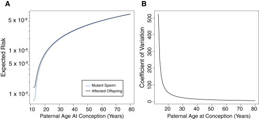
(A) Unconditional on the observation of an affected offspring, the mean proportion of mutant sperm and the expected risk of a first affected offspring (the sum of sperm and egg) are presented over various possible paternal ages according to our model. Mutation risk increases with paternal age.

(B) Coefficient of variation of the proportion of mutant sperm as a function of paternal age. Notably, the curve sharply decreases, indicating that although the proportion of mutant gametes increases, the variability among fathers of a given age decreases in relation to the mean. For these analyses, we set λ₁ = λ₂ = 1 × 10⁻¹⁰, p = q = 0.9, α = 0.05, β = 0.05, γ = 0.05, and ξ = 0.05 (see Material and Methods). An interactive version of this analysis is available online.

Risk of a First Affected Offspring

For our analyses, we considered each mitosis as equally likely to result in a mutation, although our framework is not limited in this regard. By varying the per-mitosis mutation rate (λ), we were able to effectively model mutations that cause sporadic genetic diseases with a variety of prevalence rates. As an example, parameterizing λ = 1 × 10⁻¹⁰ resulted in an expected proportion of offspring harboring a mutation of 2.06 × 10⁻⁸ in a mating with a 30-year-old male, which is consistent with previous estimates of human mutation rates per base pair per generation.^18,19 Studies using massively parallel sequencing have identified a strong paternal bias in the origin of new mutations, which increases with age.¹⁰ Our modeling suggests that additional mitoses during spermatogenesis are a potential source of this bias, as previously hypothesized (Figure 2A).¹⁰ Because female gametes do not undergo mitosis after birth, risk of SNVs and nonrecurrent CNVs is not predicted to vary with maternal age.¹⁰

Interestingly, the variance of the proportion of mutants is relatively stable with paternal age. However, the expectation of the proportion is steadily increasing. Therefore, the coefficient of variation, defined as the ratio of the standard deviation to the expectation, decreases as a father ages (Figure 2B). This finding has direct consequences for recurrence risk as we update our expectation of the proportion of mutants on the basis of the observation of an affected child.

Recurrence Risk

Recurrence risk in the context of a new transmitted mutation is defined as the chance that parents will have a second child harboring the same DNA mutation as a previous child. Analysis of recurrence risk must consider two distinct underlying biological processes that can lead to recurrence: (1) when a mutation arises and is maintained in the lineage of clonally related cells ancestral to a mutant sperm or egg and (2) when an identical mutation arises more than once within the developing germ cells across multiple clonal sublineages. The contribution of the latter is highly influenced by the per-mitosis mutation rate of the given variant, but for most estimates of mutation rate, the contribution of independent mutations to recurrence risk is negligible. Therefore, our analysis of recurrence considered the clonal development, persistence, and selective forces²⁰ on germ cells and the propagation of mutations within these clonal lineages.

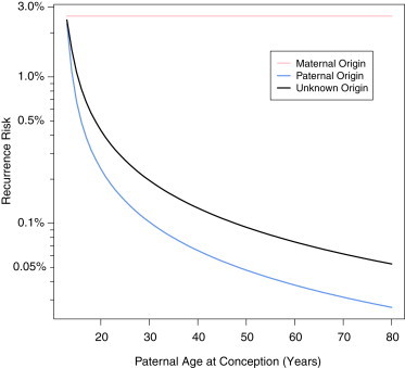
Our results show that recurrence risk depends on the parent of origin of the transmitted mutation. For maternally transmitted mutations, recurrence risk is considerably higher than empiric estimates for autosomal-dominant conditions but is consistent with observations for X-linked recessive disease (Tables 1 and 2). For paternally transmitted mutations, recurrence risk is similar overall to empirical risk estimates; however, the analyses revealed that paternal age is an important variable modifying recurrence risk. For young fathers who transmit a mutant gamete, recurrence risk is determined to be considerably higher because sampling a mutant is more unexpected and corresponds to a large increase in the expected risk of additional transmission (Figure 3). However, recurrence risk decreases with paternal age because observation of a transmitted mutation is more consistent with the expected increase in mutations in the paternal germ pool. In many real-life situations, knowledge of the parent of origin of new mutations is unavailable. In this circumstance, analysis of recurrence risk must consider the asymmetry in the parent of origin of new mutations. In this case, we calculate the recurrence risk by multiplying the sum of the risk for each parent by the probability that the sampled mutation was transmitted from that parent (Figure 3).

Table 2.

Selected Recurrence-Risk Estimates Calculated from Our Analyses

Parent	Age	Mosaic in Blood	Recurrence-Risk Estimates
			Risk Haplotype				Unknown Haplotype
			One Affected and Zero Unaffected	One Affected and One Unaffected	Two Affected and Zero Unaffected	Three Affected and Zero Unaffected	One Affected and One Unaffected
Mother	any	unknown	2.60%	2.48%	4.95%	7.07%	2.54%
Father	20	unknown	0.235%	0.234%	0.468%	0.699%	0.235%
Father	25	unknown	0.142%	0.142%	0.28%	0.42%	0.142%
Father	30	unknown	0.102%	0.102%	0.203%	0.305%	0.102%
Father	35	unknown	0.080%	0.079%	0.159%	0.238%	0.080%
Father	40	unknown	0.065%	0.065%	0.130%	0.195%	0.065%
Father	50	unknown	0.048%	0.048%	0.096%	0.143%	0.048%
Unknown	30	unknown	0.197%	–	–	–	–
Unknown	50	unknown	0.094%	–	–	–	–
Mother	any	yes	5.21%	4.72%	9.40%	12.9%	4.96%
Father	any	yes	5.21%	4.72%	9.40%	12.9%	4.96%

Information gained about recurrence risk from observation of unaffected offspring depends on the chromosome haplotype inherited from the parent who transmitted the mutant allele to the affected offspring. Inheriting the chromosome on which the mutation occurred (the risk haplotype) but with a wild-type allele provides much more information than inheriting the homologous chromosome’s haplotype. Absence of evidence of somatic mosaicism is treated as unknown because only a subset of tissue can be tested. Updating recurrence risk on the basis of additional offspring for an unknown transmitting parent is not considered in this manuscript. We caution against using this model-based table directly in clinical practice.

Figure 3.

Analysis of Recurrence Risk as a Function of Parent of Origin and Paternal Age

Because oogenesis completes during embryogenesis, recurrence risk of maternally transmitted mutations is not expected to vary with maternal age. According to our model, recurrence risk of paternally transmitted mutations steadily decreases with age, despite an increasing risk of a first affected offspring. When the parent of origin is unknown, the overall recurrence risk is the probability-weighted sum of the recurrence risks for both parents. An interactive version of this analysis is available online.

The birth of additional offspring, either affected or unaffected, provides additional insight into the number of mutant gametes in the germ pool of the transmitting parent. Importantly, the information derived from unaffected offspring depends on the haplotype that they inherited from the transmitting parent. Inheriting the same haplotype as the affected sibling but with a wild-type allele provides information about the frequency of mutant diploid germ cells. Inheritance of the haplotype from the homologous parental chromosome provides almost no information. Table 2 lists posterior recurrence-risk estimates based on a Beta-Binomial Bayesian formulation (see Material and Methods) for a number of potential family structures. For transmitting mothers, the observation of a second affected offspring raises the recurrence risk of a third affected offspring to a potentially clinically actionable level. However, for transmitting fathers, risk of a third affected offspring is still less than 1% according to our model. Surprisingly, when information of an unexpected recurrence from an unknown parent is incorporated, the paternal bias of new mutations disappears and each parent is equally likely to have transmitted the mutation.

Parental Somatic Mosaicism and Recurrence Risk

Somatic mosaicism is the presence of a mutation in a subset of body tissues other than, or in addition to, the germline.²¹ Our previous studies suggest that parental somatic mosaicism for transmitted mutations (at least for nonrecurrent CNV alleles) is more common than previously identified and occurs at a rate of ∼4%.⁴ Detecting somatic mosaicism in a transmitting parent—for example, in peripheral blood—provides information regarding the timing of a mutation because the germline becomes segregated from the rest of the embryo within the first 15 mitoses.^22,23 According to our analysis, compared to mutations for which no information is known, mutations that are also somatically mosaic in the transmitting parent are twice as likely to recur for mothers and, surprisingly, 51× more likely to recur in 30-year-old fathers (Table 2). For most reasonable mutation rates and paternal ages, somatically mosaic parents of either sex are at roughly equivalent risks of recurrence. Although definitively determining that mutant cells are exclusively confined to the parental germline is not experimentally feasible, our analyses suggest that recurrence risk for such parents is 2–3 orders of magnitude lower than that for parents with mutations that occurred before the segregation of the germline.

Recurrence-Risk Calculator

To make our analyses more accessible, we developed an online tool to explore how changes in parameters of the model and parent of origin influence estimates of recurrence. The parameters used for Table 2 are provided as the default. This tool is detailed in the Web Resources and might help to conceptualize the complex interplay among the factors that determine gametogenesis. Nonetheless, across a wide parameter space, the major conclusions remain: parent of origin and somatic mosaicism are major determinants of recurrence risk.

Discussion

Estimating recurrence risk is an important clinical concept that directly affects the medical management and reproductive choices of couples with children affected by genetic disease. Geneticists and genetic counselors often rely on empirical understanding of recurrence risk, but specific information is available for only the most common and well-understood diseases. Thus, frequently, they can only advise on the basis of experience with a broad spectrum of diseases and mutation types. Our analyses yield new insights into recurrence and implicate the parent of origin as a central variable in the analysis of risk, but we caution against using these estimates directly in routine clinical practice. Nonetheless, we have found that mutations of maternal origin determine higher recurrence risk than do paternal mutations. The analysis that underlies this finding requires detailed consideration of the fundamental developmental processes that lead to the transmission of new mutations. A comprehensive mathematical treatment of recurrence risk in humans is not available in the literature, and the authoritative reference does not consider the complexity of sampling stochastic clonal expansion or spermatogonial self-renewal.²⁴ Other studies have considered the consequences of mosaicism (also called “premeiotic clusters”) but were directed more toward the study of population genetics.^3,25,26

Our model predictions are consistent with the unexplained observation of increased recurrence risk among X-linked recessive diseases. This elevated recurrence risk is not a feature of a special choice of parameters in our model but is instead a result of the structural difference in gametogenesis between the sexes. For females, mutations during the clonal-expansion phase are rare, but the observation of a transmitted mutation is a strong indication that the maternal germline is rich in mutant gametes. In probabilistic terms, although the expected proportion of mutants is quite small, the prior variance in the proportion is quite large. Subsequently, the observation of a transmitted mutation has considerable information to update and increase the expected proportion of mutants in the maternal germ pool.

The situation for males is different. According to our model, and consistent with observations, the expected proportion of mutants is higher in males and steadily increases with age. However, our analyses show that the coefficient of variation of this proportion of mutants is modest and steadily decreases with paternal age. As such, observation of a transmitted mutation does not shift the expectation of the fraction of mutants in the sperm pool as strongly as for female germ cells. Observation of a transmitted mutation from the paternal side contains comparatively less information to alter the expected risk of recurrence.

Our model framework permits us to analyze the impact of mosaicism on recurrence risk. Emerging evidence suggests that parental somatic mosaicism for transmitted mutations is more common than previously thought and might have a clinically significant impact on recurrence risk. Our results indicate that compared to observation of a transmission alone, observation of somatic mosaicism increases recurrence risk 2-fold in mothers and more than 50-fold in fathers.

The conclusions of our model can be tested by analysis of the parent of origin and parental mosaicism in families where transmitted genetic disease is caused by new mutations, including families with and without observed recurrences. Although these analyses are not commonly performed, our results suggest that identification of the parent of origin is a key consideration for intrafamilial recurrence risk. In the absence of genome-wide data that permit phasing of the mutant allele, personalized assays such as single-gene sequencing or customized PCR to determine the parent of origin might be useful. Likewise, parental somatic mosaicism can be molecularly identified,⁸ and techniques with improved sensitivity should also be developed.

In addition to somatic-mosaicism status and parent of origin, the type of mutation in question most likely influences the parameters determining recurrence risk. The so-called “paternal-age effect” disorders²⁰ provide particularly prominent examples. The high prevalence of Apert syndrome is attributed to mutant spermatogonial stem cells dividing more frequently than wild-type cells.¹⁷ Although the analysis we present in the text does not address this type of effect, our model and online explorer (see Web Resources) have provisions to modify these parameters. Likewise, some mutation types, such as CpG dinucleotide transitions or CNVs, might occur at higher or lower rates in spermatogonial stem cells or vary by sex. Moreover, genetic diversity in individual parents might influence mutation rate globally²⁷ or for select mutation types during mitosis, as has been observed for meiotic mutational mechanisms.²⁸ Our model can also accommodate inquiry into these aspects of human variation.

We suggest that our modeling framework is flexible and that our results are robust across many choices of parameters of mutation rate and cellular fitness. However, our modeling framework does not account for all sources of new disease-causing mutations. Importantly, we do not consider meiotic-origin mutations, such as nondisjunction events that mediate aneuploidy. As such, disorders such as Down syndrome and other conditions associated with increasing maternal age are not the focus of our work.

Other classes of deleterious mutations could cause recurrent disease under more complex patterns of inheritance. Our modeling is focused on autosomal-dominant alleles, in which a single copy of a mutant allele determines disease state. This model is also directly applicable for computing recurrence risk for X-linked recessive disease. In other unexpected recurrence situations involving new mutations, disease occurs through compound heterozygosity, in which a new mutation from one parent is randomly paired with a nonfunctional recessive allele inherited from the other parent. In these situations, familial recurrence rates would be half of what is predicted by our model, given that disease recurrence requires the nonfunctional familial allele from the other parent to also be transmitted to the offspring. Although our analysis focused on the inheritance of new mutations for couples, it might also contribute to understanding apparent violations of Mendelian expectations in some pedigrees.

In addition to their immediate applicability to recurrence risk of new mutations, our analytic results also represent a technical advance in the theory of branching processes. We extend the exact sampling formulas for multitype Galton-Watson processes to multiphase models, which in this application permitted us to consider both clonal-expansion and self-renewal phases of gametogenesis. This advance might extend the application of Galton-Watson models and sampling results to other contexts in biology, such as population genetics or the emergence of mutations in model organisms that can be experimentally assayed.²⁹ We also developed an interesting result concerning the analysis of stochastic proportions. We showed that sampling a rare particle updates the expected proportion of that rare particle to the value determined by the size-biased distribution of the proportion. This general fact could have other uses in statistics and probability.

Our modeling framework considers only two types, wild-type and mutants. This simplifying choice is appropriate for the analysis of recurrent transmission of an index mutation within a family. We recognize that additional work is required for considering the full spectrum of variation that can emerge during clonal divisions and ultimately be transmitted by gametes between generations. We suggest that the basic structure of our model can be extended to considering an arbitrary number of mutation types. The framework of our model is to allow new mutants to arise and reproduce starting from a parental cell type. If we iterate this approach, allowing mutant cells from our model to initiate additional compound mutant lineages, then the basic mathematical structure as presented in Appendices A and B can be extended to considering arbitrary accumulation of mutations as well as back mutation. Future work in this area could advance the understanding of clonal heterogeneity, potentially of use in the study of malignancy.

Our results suggest that parent of origin and somatic-mosaicism status have considerable utility to inform estimation of recurrence risk. Our results naturally raise the question, “should clinicians quote a value different than <1%”? Empirical evidence,⁸ together with our model, suggests that for some clearly defined mutations, on average, risk is considerably higher. Large-scale empirical studies of parent of origin, parental somatic mosaicism, and mutational mechanisms are required for fully understanding recurrence risk. For any particular mutation, the interplay between these contributory factors determines risk, but their superposition makes it difficult to disentangle them. Further modeling based on improved empirical data would be an excellent approach. Nonetheless, we suggest that for families most concerned about recurrence, particularly those with younger fathers, investigations into parent of origin and mosaicism can help to reassure, improve family planning, or direct the potential use of preimplantation or prenatal genetic diagnostics.

Appendix A: Exact Formulas for Mutant Proportions in the Paternal Germline

A Two-Phase Model of Gametogenesis

This study considers sexual dimorphism in gametogenesis, mosaicism, and the consequences of these phenomena for mutation transmission between parents and offspring. Although we are considering diploid cells that precede the formation of haploid gametes, we consider cells as a whole rather than each homologous chromosome separately. Under this scheme, a cell with at least one mutation at a given locus is considered mutant, whereas a cell with only wild-type copies of DNA at that locus is considered wild-type. This simplification is reasonable for low mutation rates because the chance that two identical variations will arise on each of the homologs in a cellular lineage is extremely low.

For a single locus, the dynamics of this process can be modeled with only two types: wild-type and mutant. Our previous work¹² provides exact sampling formulas for a single-phase two-type Galton-Watson model of clonal expansion with mutation, and this model is suitable to represent the female germline. Here, we extend our analyses to consider a two-stage, two-type Galton-Watson process suitable to represent the male germline. By two-stage we mean that the progeny distributions start according to the clonal-expansion rules as used in our earlier work but then switch at a fixed generation j from clonal expansion to self-renewal, under which the overall population size of the germ pool remains relatively stable. This self-renewal process proceeds for n − j = k generations. This two-stage model of expansion followed by an extended period of self-renewal reflects the characteristics of the male germline. The formulas for the model initiated from a single wild-type cell at generation 0 are presented below. In what follows, we define wild-type cells as type 0 and mutants as type 1.

Probability Generating Functions

The fundamental tool for analysis of Galton-Watson branching processes is the probability generating function (pgf). A pgf is a polynomial transformation used to represent a discrete probability distribution. The real valued arguments to pgfs are “dummy variables,” where powers of these arguments correspond to the possible values of the discrete random variable whose distribution is being analyzed. The coefficient of each polynomial term corresponds to the probability that the random variable being modeled takes on the values indexed in the exponents. For instance, for a variable X taking on the values {0,1,2}, let ϕ(u) be the pgf of X. We could write ϕ(u) = 0.25 + 0.5u + 0.25u², indicating that X takes the value 0 with probability 0.25, the value 1 with probability 0.5, and the value 2 with probability 0.25. Joint distributions of two or more random variables can be similarly modeled with bivariate or multivariate pgfs. For instance, for the pair of random variables X and Y, each taking on values in {0,1,2}, we could write ϕ(u,v) = 0.25 + 0.5uv + 0.25u², modeling a bivariate distribution where the only allowed values of the ordered pair (X,Y) are (0,0), (1,1), and (2,0) and where (1,1) occurs with probability 0.5.

The benefit of this notation is that various properties of discrete distributions can be determined by analytic properties of the pgf. For instance, the distribution of sums of independent discrete random variables can be analyzed by products of pgfs, and for multitype branching processes, function composition of the pgfs for the progeny determines the distribution of the evolution of the process.

Using pgfs in Our Two-Phase Model

In our previously published work,¹² we defined progeny pgfs for the clonal-expansion process. ϕ₀ represents the offspring of a wild-type cell, and ϕ₁ is the pgf for the offspring of a mutant cell. The bivariate pgfs for wild-type (dummy variable u) and mutant cells (v) during clonal expansion are the following:

$${\varphi }_0\left(u,v\right)=1-p+p\lambda uv+p\left(1-\lambda \right)u^2$$ (Equation A1)

$${\varphi }_1\left(u,v\right)=1-q+q{v}^2.$$ (Equation A2)

Wild-type cells double with probability p or expire with no progeny with probability 1 − p. Independently, dividing wild-type cells could either produce two wild-types with probability 1 − λ or give rise to one wild-type and one mutant with probability λ. Mutant cells can only give rise to two additional mutants with probability q or die without division with probability 1 − q.

The process of spermatogonial self-renewal proceeds by asymmetric cell division, in which spermatogonial cells most often produce a single renewal cell and only rarely double or expire with no progeny. As in clonal expansion, mutant cells can give rise to mutants, whereas wild-types can produce either wild-type or mutant offspring. We define the pgfs for the self-renewal process as ψ₀ for wild-type and ψ₁ for mutant spermatogonial cells:

$${\psi }_0\left(u,v\right)=1-\alpha -\beta +\alpha u^2+\beta \lambda v+\beta \left(1-\lambda \right)u$$ (Equation A3)

$${\psi }_1\left(u,v\right)=1-\gamma -\xi +\gamma v^2+\xi v.$$ (Equation A4)

Wild-type spermatogonial cells self-renew with probability β(1 − λ), divide with probability α, and expire with probability 1 − α − β. They generate mutant spermatogonial cells with probability βλ. Similarly, for mutant spermatogonial cells, they self-renew with probability ξ, divide with probability γ, and expire with probability 1 − γ − ξ.

As discussed above, male germline gametogenesis can be modeled by iterative composition of these progeny pgfs. The two-stage process has a total pgf that combines the j-fold compositions of the first-stage expansion process with n − j = k-fold composition of the second-stage self-renewal process. As a reminder, we use the Greek letter ϕ for the first-stage expansion-phase pgf and the letter ψ for the second-stage of self-renewal. By ${\psi }_0^{\left(k\right)}$ we intend the k-fold composition of the second-stage process starting from a single wild-type cell, and ${\varphi }_0^{\left(j\right)}$ is the j-fold composition of the expansion phase; we use the subscript 1 for the corresponding functions beginning from mutants. ${\pi }_0^{\left(n\right)}$ represents the total pgf for the two-stage process starting from a single wild-type cell, whereas ${\pi }_1^{\left(n\right)}$ is the corresponding function for a process initiated by a mutant:

$${\pi }_0^{\left(n\right)}\left(u,v\right)={\varphi }_0^{\left(j\right)}\left({\psi }_0^{\left(k\right)}\left(u,v\right),{\psi }_1^{\left(k\right)}\left(u,v\right)\right)$$ (Equation A5)

$${\pi }_1^{\left(n\right)}\left(u,v\right)={\varphi }_1^{\left(j\right)}\left({\psi }_0^{\left(k\right)}\left(u,v\right),{\psi }_1^{\left(k\right)}\left(u,v\right)\right).$$ (Equation A6)

According to our prior work,¹² if we let $Z_n^0$ and $Z_n^1$ be the number of wild-type and mutant cells, respectively, at generation n, then the mean and variance of the proportion of mutants in this two-stage process can be determined with the first and second derivatives of the bivariate pgf. The expression for the expected proportion of mutants is

$$E\left[\frac{Z_n^1}{Z_n^0+Z_n^1}|Z_n^0+Z_n^1>0\right]=\frac{1}{1-{\pi }_0^{\left(n\right)}\left(\mathrm{0,0}\right)}{\int }_0^1\frac{\partial }{\partial v}{\pi }_0^{\left(n\right)}{\left(u,v\right)|}_{u=v=s}ds.$$ (Equation A7)

A related expression involving second derivatives determines the variance. Applying the chain rule to consider the first derivatives, we have

$$\frac{\partial {\pi }_0^{\left(n\right)}}{\partial v}\left(u,v\right)=\frac{\partial {\varphi }_0^{\left(j\right)}}{\partial {\psi }_0^{\left(k\right)}}\frac{\partial {\psi }_0^{\left(k\right)}}{\partial v}+\frac{\partial {\varphi }_0^{\left(j\right)}}{\partial {\psi }_1^{\left(k\right)}}\frac{\partial {\psi }_1^{\left(k\right)}}{\partial v}$$ (Equation A8)

$$\frac{\partial {\pi }_1^{\left(n\right)}}{\partial v}\left(u,v\right)=\frac{\partial {\varphi }_1^{\left(j\right)}}{\partial {\psi }_0^{\left(k\right)}}\frac{\partial {\psi }_0^{\left(k\right)}}{\partial v}+\frac{\partial {\varphi }_1^{\left(j\right)}}{\partial {\psi }_1^{\left(k\right)}}\frac{\partial {\psi }_1^{\left(k\right)}}{\partial v}.$$ (Equation A9)

The chain rule shows that the total derivative requires determination of derivatives for both wild-type and mutant cells in both the first- and second-stage processes. Similarly, computing second derivatives, as required for the variance determination, also depends on differentiating both pgfs for both stages. The derivatives for the first stage are available in our prior work. The derivatives for the second-stage process are determined as follows:

$${\psi }_0^{\left(0\right)}\left(u,v\right)=u$$ (Equation A10)

$${\psi }_0^{\left(1\right)}\left(u,v\right)=1-\alpha -\beta +\alpha u^2+\beta \lambda v+\beta \left(1-\lambda \right)u$$ (Equation A11)

$$\frac{\partial {\psi }_0^{\left(1\right)}}{\partial v}\left(u,v\right)=\beta \lambda$$ (Equation A12)

$$\frac{{\partial }^2{\psi }_0^{\left(1\right)}}{\partial v^2}\left(u,v\right)=0$$ (Equation A13)

$${\psi }_0^{\left(k\right)}\left(u,v\right)=1-\alpha -\beta +\alpha {\left({\psi }_0^{\left(k-1\right)}\left(u,v\right)\right)}^2+\beta \lambda {\psi }_1^{\left(k-1\right)}\left(u,v\right)+\beta \left(1-\lambda \right){\psi }_0^{\left(k-1\right)}\left(u,v\right).$$ (Equation A14)

Suppressing (u,v) on the right-hand side, we have

$$\frac{\partial {\psi }_0^{\left(k\right)}}{\partial v}\left(u,v\right)=2\alpha \left[{\psi }_0^{\left(k-1\right)}\frac{\partial {\psi }_0^{\left(k-1\right)}}{\partial v}\right]+\beta \lambda \frac{\partial {\psi }_1^{\left(k-1\right)}}{\partial v}+\beta \left(1-\lambda \right)\frac{\partial {\psi }_0^{\left(k-1\right)}}{\partial v}$$ (Equation A15)

$$\frac{{\partial }^2{\psi }_0^{\left(k\right)}}{\partial v^2}\left(u,v\right)=2\alpha \left[{\psi }_0^{\left(k-1\right)}\frac{{\partial }^2{\psi }_0^{\left(k-1\right)}}{\partial v^2}+{\left(\frac{\partial {\psi }_0^{\left(k-1\right)}}{\partial v}\right)}^2\right]+\beta \lambda \frac{{\partial }^2{\psi }_1^{\left(k-1\right)}}{\partial v^2}+\beta \left(1-\lambda \right)\frac{{\partial }^2{\psi }_0^{\left(k-1\right)}}{\partial v^2}.$$ (Equation A16)

And for mutants, we have

$${\psi }_1^{\left(0\right)}\left(u,v\right)=v$$ (Equation A17)

$${\psi }_1^{\left(1\right)}\left(u,v\right)=1-\gamma -\xi +\gamma v^2+\xi v$$ (Equation A18)

$$\frac{\partial {\psi }_1^{\left(1\right)}}{\partial v}\left(u,v\right)=2\gamma v+\xi$$ (Equation A19)

$$\frac{{\partial }^2{\psi }_1^{\left(1\right)}}{\partial v^2}\left(u,v\right)=2\gamma$$ (Equation A20)

$${\psi }_1^{\left(k\right)}\left(u,v\right)=1-\gamma -\xi +\gamma {\left({\psi }_1^{\left(k-1\right)}\right)}^2+\xi {\psi }_1^{\left(k-1\right)}$$ (Equation A21)

$$\frac{\partial {\psi }_1^{\left(k\right)}}{\partial v}\left(u,v\right)=2\gamma {\psi }_1^{\left(k-1\right)}\frac{\partial {\psi }_1^{\left(k-1\right)}}{\partial v}+\xi \frac{\partial {\psi }_1^{\left(k-1\right)}}{\partial v}$$ (Equation A22)

$$\frac{{\partial }^2{\psi }_1^{\left(k\right)}}{\partial v^2}\left(u,v\right)=2\gamma \left[{\left(\frac{\partial {\psi }_1^{\left(k-1\right)}}{\partial v}\right)}^2+{\psi }_1^{\left(k-1\right)}\frac{{\partial }^2{\psi }_1^{\left(k-1\right)}}{\partial v^2}\right]+\xi \frac{{\partial }^2{\psi }_1^{\left(k-1\right)}}{\partial v^2}.$$ (Equation A23)

To compute the integrands for the mean and variance formulas, we first compute the inner function composition for the second-stage self-renewal process and then use this as the initial condition for evaluating the composition of the first-stage clonal-expansion process. It is important to note that evaluation of these function compositions proceeds from the “inside out”; that is, the compositions proceed from the final generation of the process backward toward ancestral cells and ultimately to the single wild-type progenitor cell. The superscripts index the number of function compositions, but these compositions are computed in the reverse order from the forward indexing of cell division. Thus, it is important to track the j and k indices for a fixed n. Recall that for a self-renewal process that proceeds for k generations after j generations of clonal expansion,

$$n=j+k$$ (Equation A24)

$$k=0\dots \left(n-j\right).$$ (Equation A25)

To initialize the two-stage composition, we start with the final round of clonal expansion, composed of the total composition representing k generations of self-renewal:

$${\pi }_0^{\left(1+k\right)}\left(u,v\right)=1-p+p\lambda {\psi }_0^{\left(k\right)}\left(u,v\right){\psi }_1^{\left(k\right)}\left(u,v\right)+p\left(1-\lambda \right){\left({\psi }_0^{\left(k\right)}\left(u,v\right)\right)}^2.$$ (Equation A26)

Again suppressing (u,v) on the right-hand side, we have

$$\frac{\partial {\pi }_0^{\left(1+k\right)}}{\partial v}\left(u,v\right)=p\lambda \left[\frac{\partial {\psi }_0^{\left(k\right)}}{\partial v}{\psi }_1^{\left(k\right)}+{\psi }_0^{\left(k\right)}\frac{\partial {\psi }_1^{\left(k\right)}}{\partial v}\right]+2p\left(1-\lambda \right){\psi }_0^{\left(k\right)}\frac{\partial {\psi }_0^{\left(k\right)}}{\partial v}$$ (Equation A27)

$$\frac{{\partial }^2{\pi }_0^{\left(1+k\right)}}{\partial v^2}\left(u,v\right)=p\lambda \left[\frac{{\partial }^2{\psi }_0^{\left(k\right)}}{\partial v^2}{\psi }_1^{\left(k\right)}+2\frac{\partial {\psi }_0^{\left(k\right)}}{\partial v}\frac{\partial {\psi }_1^{\left(k\right)}}{\partial v}+{\psi }_0^{\left(k\right)}\frac{{\partial }^2{\psi }_1^{\left(k\right)}}{\partial v^2}\right]+2p\left(1-\lambda \right)\left[{\left(\frac{\partial {\psi }_0^{\left(k\right)}}{\partial v}\right)}^2+{\psi }_0^{\left(k\right)}\frac{{\partial }^2{\psi }_0^{\left(k\right)}}{\partial v^2}\right].$$ (Equation A28)

Subsequently for j>1,

$${\pi }_0^{\left(j+k\right)}\left(u,v\right)=1-p+p\lambda {\pi }_0^{\left(j+k-1\right)}{\pi }_1^{\left(j+k-1\right)}+p\left(1-\lambda \right){\left({\pi }_0^{\left(j+k-1\right)}\right)}^2$$ (Equation A29)

$$\frac{\partial {\pi }_0^{\left(j+k\right)}}{\partial v}\left(u,v\right)=p\lambda \left[\frac{\partial {\pi }_0^{\left(j+k-1\right)}}{\partial v}{\pi }_1^{\left(j+k-1\right)}+{\pi }_0^{\left(j+k-1\right)}\frac{\partial {\pi }_1^{\left(j+k-1\right)}}{\partial v}\right]+2p\left(1-\lambda \right){\pi }_0^{\left(j+k-1\right)}\frac{\partial {\pi }_0^{\left(j+k-1\right)}}{\partial v}$$ (Equation A30)

$$\frac{{\partial }^2{\pi }_0^{\left(j+k\right)}}{\partial v^2}\left(u,v\right)=p\lambda \left[\frac{{\partial }^2{\pi }_0^{\left(j+k-1\right)}}{\partial v^2}{\pi }_1^{\left(j+k-1\right)}+2\frac{\partial {\pi }_0^{\left(j+k-1\right)}}{\partial v}\frac{\partial {\pi }_1^{\left(j+k-1\right)}}{\partial v}+{\pi }_0^{\left(j+k-1\right)}\frac{{\partial }^2{\pi }_1^{\left(j+k-1\right)}}{\partial v^2}\right]+2p\left(1-\lambda \right)\left[{\left(\frac{\partial {\pi }_0^{\left(j+k-1\right)}}{\partial v}\right)}^2+{\pi }_0^{\left(j+k-1\right)}\frac{{\partial }^2{\pi }_0^{\left(j+k-1\right)}}{\partial v^2}\right].$$ (Equation A31)

Again for mutants,

$${\pi }_1^{\left(1+k\right)}\left(u,v\right)=1-q+q{\left({\psi }_1^{\left(k\right)}\right)}^2$$ (Equation A32)

$$\frac{\partial {\pi }_1^{\left(1+k\right)}}{\partial v}\left(u,v\right)=2q{\psi }_1^{\left(k\right)}\frac{\partial {\psi }_1^{\left(k\right)}}{\partial v}$$ (Equation A33)

$$\frac{{\partial }^2{\pi }_1^{\left(1+k\right)}}{\partial v^2}\left(u,v\right)=2q{\left(\frac{\partial {\psi }_1^{\left(k\right)}}{\partial v}\right)}^2+2q{\psi }_1^{\left(k\right)}\frac{{\partial }^2{\psi }_1^{\left(k\right)}}{\partial v^2}$$ (Equation A34)

$${\pi }_1^{\left(j+k\right)}\left(u,v\right)=1-q+q{\left({\pi }_1^{\left(j+k-1\right)}\right)}^2$$ (Equation A35)

$$\frac{\partial {\pi }_1^{\left(j+k\right)}}{\partial v}\left(u,v\right)=2q{\pi }_1^{\left(j+k-1\right)}\frac{\partial {\pi }_1^{\left(j+k-1\right)}}{\partial v}$$ (Equation A36)

$$\frac{{\partial }^2{\pi }_1^{\left(j+k\right)}}{\partial v^2}\left(u,v\right)=2q{\left(\frac{\partial {\pi }_1^{\left(j+k-1\right)}}{\partial v}\right)}^2+2q{\pi }_1^{\left(j+k-1\right)}\frac{{\partial }^2{\pi }_1^{\left(j+k-1\right)}}{\partial v^2}.$$ (Equation A37)

Recursive Scheme for Pointwise Function Evaluation

Expansion of the polynomials defined above by recursive function composition proves impractical. As in our previous work,¹² we developed a recursive scheme for pointwise function evaluation to permit numerical evaluation of the integrand for determining the exact mean and variance of the mutant proportion. We define this notation here:

$$H_k\left(s\right)={\psi }_0^{\left(k\right)}\left(s,s\right),h_k\left(s\right)=\frac{\partial {\psi }_0^{\left(k\right)}}{\partial v}{\left(u,v\right)|}_{u=v=s},h{h}_k\left(s\right)=\frac{{\partial }^2{\psi }_0^{\left(k\right)}}{\partial v^2}{\left(u,v\right)|}_{u=v=s}$$ (Equations A38)

$$M_k\left(s\right)={\psi }_0^{\left(k\right)}\left(s,s\right),m_k\left(s\right)=\frac{\partial {\psi }_1^{\left(k\right)}}{\partial v}{\left(u,v\right)|}_{u=v=s},m{m}_k\left(s\right)=\frac{{\partial }^2{\psi }_1^{\left(k\right)}}{\partial v^2}{\left(u,v\right)|}_{u=v=s}$$ (Equations A39)

$$F_j\left(s\right)={\varphi }_0^{\left(j\right)}\left(s,s\right),f_j\left(s\right)=\frac{\partial {\varphi }_0^{\left(j\right)}}{\partial v}{\left(u,v\right)|}_{u=v=s},f{f}_j\left(s\right)=\frac{{\partial }^2{\varphi }_0^{\left(j\right)}}{\partial v^2}{\left(u,v\right)|}_{u=v=s}$$ (Equations A40)

$$G_j\left(s\right)={\varphi }_0^{\left(j\right)}\left(s,s\right),g_j\left(s\right)=\frac{\partial {\varphi }_1^{\left(j\right)}}{\partial v}{\left(u,v\right)|}_{u=v=s},g{g}_j\left(s\right)=\frac{{\partial }^2{\varphi }_1^{\left(j\right)}}{\partial v^2}{\left(u,v\right)|}_{u=v=s}.$$ (Equations A41)

We obtain the following recursive scheme:

$$H_k\left(s\right)=1-\alpha -\beta +\alpha H_{k-1}^2\left(s\right)+\beta \lambda M_{k-1}\left(s\right)+\beta \left(1-\lambda \right)H_{k-1}\left(s\right)$$ (Equation A42)

$$h_k\left(s\right)=2\alpha \left[H_{k-1}\left(s\right)h_{k-1}\left(s\right)\right]+\beta \lambda m_{k-1}\left(s\right)+\beta \left(1-\lambda \right)h_{k-1}\left(s\right)$$ (Equation A43)

$$h{h}_k\left(s\right)=2\alpha \left[H_{k-1}\left(s\right)h{h}_{k-1}\left(s\right)+h_{k-1}^2\left(s\right)\right]+\beta \lambda m{m}_{k-1}\left(s\right)+\beta \left(1-\lambda \right)h{h}_{k-1}\left(s\right)$$ (Equation A44)

$$M_k\left(s\right)=1-\gamma -\xi +\gamma M_{k-1}^2\left(s\right)+\xi M_{k-1}\left(s\right)$$ (Equation A45)

$$m_k\left(s\right)=2\gamma M_{k-1}\left(s\right)m_{k-1}\left(s\right)+\xi m_{k-1}\left(s\right)$$ (Equation A46)

$$m{m}_k\left(s\right)=2\gamma \left[m_{k-1}^2\left(s\right)+M{k}_{k-1}\left(s\right)m{m}_{k-1}\left(s\right)\right]+\xi m{m}_{k-1}\left(s\right)$$ (Equation A47)

$$F_j\left(s\right)=1-p+p\lambda F_{j-1}\left(s\right)G_{j-1}\left(s\right)+p\left(1-\lambda \right)F_{j-1}^2\left(s\right)$$ (Equation A48)

$$f_j\left(s\right)=p\lambda \left[f_{j-1}\left(s\right)G_{j-1}\left(s\right)+F_{j-1}\left(s\right)g_{j-1}\left(s\right)\right]+2p\left(1-\lambda \right)F_{j-1}\left(s\right)f_{j-1}\left(s\right)$$ (Equation A49)

$$f{f}_j\left(s\right)=p\lambda \left[f{f}_{j-1}\left(s\right)G_{j-1}\left(s\right)+2f_{j-1}\left(s\right)g_{j-1}\left(s\right)+F_{j-1}\left(s\right)g{g}_{j-1}\left(s\right)\right]+2p\left(1-\lambda \right)\left[f_{j-1}^2\left(s\right)+F_{j-1}\left(s\right)f{f}_{j-1}\left(s\right)\right]$$ (Equation A50)

$$G_j\left(s\right)=1-q+q{G}_{j-1}^2\left(s\right)$$ (Equation A51)

$$g_j\left(s\right)=2q{G}_{j-1}\left(s\right)g_{j-1}\left(s\right)$$ (Equation A52)

$$g{g}_j\left(s\right)=2q\left[g_{j-1}^2\left(s\right)+G_{j-1}\left(s\right)g{g}_{j-1}\left(s\right)\right]\text{.}$$ (Equation A53)

The initial conditions are

$$H_1\left(s\right)=1-\alpha -\beta +\alpha s^2+\beta s$$ (Equation A54)

$$h_1\left(s\right)=\beta \lambda$$ (Equation A55)

$$h{h}_1\left(s\right)=0$$ (Equation A56)

$$M_1\left(s\right)=1-\gamma -\xi +\gamma s^2+\xi s$$ (Equation A57)

$$m_1\left(s\right)=2\gamma s+\xi$$ (Equation A58)

$$m{m}_1\left(s\right)=2\gamma$$ (Equation A59)

$$F_1\left(s\right)=1-p+p{H}_k^2\left(s\right)$$ (Equation A60)

$$f_1\left(s\right)=p\lambda \left[h_k\left(s\right)M_k\left(s\right)+H_k\left(s\right)m_k\left(s\right)\right]+2p\left(1-\lambda \right)H_k\left(s\right)h_k\left(s\right)$$ (Equation A61)

$$f{f}_1\left(s\right)=p\lambda \left[h{h}_k\left(s\right)M_k\left(s\right)+2h_k\left(s\right)m_k\left(s\right)+H_k\left(s\right)m{m}_k\left(s\right)\right]+2p\left(1-\lambda \right)\left[h_k^2\left(s\right)+H_k\left(s\right)h{h}_k\left(s\right)\right]$$ (Equation A62)

$$G_1\left(s\right)=1-q+q{M}_k^2\left(s\right)$$ (Equation A63)

$$g_1\left(s\right)=2q{M}_k\left(s\right)m_k\left(s\right)$$ (Equation A64)

$$g{g}_1\left(s\right)=2q{m}_k^2\left(s\right)+2q{M}_k\left(s\right)m{m}_k\left(s\right).$$ (Equation A65)

For the female line composed of only clonal expansion, the initial conditions are

$$F_1\left(s\right)=1-p+p{s}^2$$ (Equation A66)

$$f_1\left(s\right)=p\lambda s$$ (Equation A67)

$$f{f}_1\left(s\right)=0$$ (Equation A68)

$$G_1\left(s\right)=1-q+q{s}^2$$ (Equation A69)

$$g_1\left(s\right)=2qs$$ (Equation A70)

$$g{g}_1\left(s\right)=2q.$$ (Equation A71)

Mathematica code implementing these recurrences can be found on our website. We note that the spermatogonial self-renewal model can be extended to allow mutation at spermatogonial division:

$${\psi }_0\left(u,v\right)=1-\alpha -\beta +\left(1-\lambda \right)\alpha u^2+\lambda \alpha uv+\beta \lambda v+\beta \left(1-\lambda \right)u.$$ (Equation A72)

We elected not to use this form for two reasons: (1) the main dynamics of the model are not substantively altered, and (2) we wished to conform with the simulation model used in our previously published work.⁴ Likewise, λ can be modeled to take on different values in the two phases of gametogenesis or vary by generation of cell division.

Appendix B: Taylor Approximations to the Moments of the Proportion of Mutants

Calculating the numerical integration of the formulas presented in Appendix A proves difficult. Approximations of the mean and variance of the proportion of mutants can be obtained with Taylor approximations of the moments of functions of random variables. In order to apply these approximations, we require the mean, variance, and covariance of the number of wild-type and mutant cells in each generation. In this problem, there are seven fundamental parameters that are determined from the progeny pgfs, and these are given in Table B1 below:

Table B1.

Model Parameter Determined by the Progeny Generating Function

Parameter	Description
μ00	expected wild-types born to a wild-type
μ01	expected mutants born to a wild-type
μ11	expected mutants born to a mutant
${\sigma }_{00}^2$	variance of wild-types born to a wild-type
${\sigma }_{01}^2$	variance of mutants born to a wild-type
${\sigma }_{11}^2$	variance of mutants born to a mutant
ρ01	the expectation of the product of the number of wild-types and mutants born to a wild-type

Importantly, the key structure of the model—where mutants can give additional mutants but wild-types make wild-types or mutants—is unchanged between the clonal-expansion and self-renewal phases. Depending on the previous generation, a single homogenous, linear recurrence in five-state variables determines the two means, the two variances, and the covariance of the number of wild-type and mutant cells in each generation. Specifying the initial state (the number of wild-type and mutant cells at the first generation) and the values of the parameters described above determines the evolution of the process. Let $Z_n^0$ be the number of wild-type cells in generation n and $Z_n^1$ be the number of mutants at n. Let ${\mathbf{Z}}_{\mathbf{n}}={\left(Z_n^0,Z_n^1\right)}^t$. We obtain

$$E\left[Z_n^0\right]=E\left[E\left[Z_n^0|Z_{n-1}^0\right]\right]=u_{00}E\left[Z_{n-1}^0\right]$$ (Equation B1)

$$V\left[Z_n^0\right]=E[V\left[Z_n^0|Z_{n-1}^0\right]]+V\left[E\left[Z_n^0|Z_{n-1}^0\right]\right]=E\left[Z_{n-1}^0\right]{\sigma }_{00}^2+{\mu }_{00}^{2}V\left[Z_{n-1}^0\right]\text{.}$$ (Equation B2)

Similarly, for $Z_n^1$ we have

$$E\left[Z_n^1\right]=E\left[E\left[Z_n^1|Z_{n-1}^0,Z_{n-1}^1\right]\right]=u_{01}E\left[Z_{n-1}^0\right]+u_{11}E\left[Z_{n-1}^1\right]$$ (Equation B3)

$$V\left[Z_n^1\right]=V\left[E\left[Z_n^1|Z_{n-1}^0,Z_{n-1}^1\right]\right]+E\left[V\left[Z_n^1|Z_{n-1}^0,Z_{n-1}^1\right]\right]={\sigma }_{01}^{2}E\left[Z_{n-1}^0\right]+{\mu }_{01}^{2}V\left[Z_{n-1}^0\right]+{\sigma }_{11}^{2}E\left[Z_{n-1}^1\right]+{\mu }_{11}^{2}V\left[Z_{n-1}^1\right]\text{.}$$ (Equation B4)

Finally, for the covariance, we have this identity:

$$Cov\left[Z_n^0,Z_n^1\right]=E\left[Cov\left[Z_n^0,Z_n^1|{\mathbf{Z}}_{n-1}\right]\right]+Cov\left[E\left[Z_n^0|{\mathbf{Z}}_{n-1}\right],E\left[Z_n^1|{\mathbf{Z}}_{n-1}\right]\right]=\left({\rho }_{01}-{\mu }_{00}{\mu }_{01}\right)E\left[Z_{n-1}^0\right]+{\mu }_{00}{\mu }_{01}V\left[Z_{n-1}^0\right]+{\mu }_{00}{\mu }_{11}Cov\left[Z_{n-1}^0,Z_{n-1}^1\right]\text{.}$$ (Equation B5)

Examining these recurrence formulas for generation n, we observe that they are homogeneous, first-order linear recurrences that depend only on the values of the previous generation, n − 1. Therefore, we can simplify and write a matrix expression for the vector: ${\mathit{\beta }}_n={\left(E\left[Z_n^0\right],V\left[Z_n^0\right],E\left[Z_n^1\right],V\left[Z_n^1\right],Cov\left[Z_n^0,Z_n^1\right]\right)}^t$.

$${\mathit{\beta }}_n=\mathbf{A}{\mathit{\beta }}_{n-1}$$ (Equation B6)

$$\mathbf{A}=\left[\begin{array}{ccccc}{\mu }_{00}& 0& 0& 0& 0\\ {\sigma }_{00}^2& {\mu }_{00}^2& 0& 0& 0\\ {\mu }_{01}& 0& {\mu }_{11}& 0& 0\\ {\sigma }_{01}^2& {\mu }_{01}^2& {\sigma }_{11}^2& {\mu }_{11}^2& 0\\ \left({\rho }_{01}-{\mu }_{00}{\mu }_{01}\right)& {\mu }_{00}{\mu }_{01}& 0& 0& {\mu }_{00}{\mu }_{11}\end{array}\right]$$ (Equation B7)

Because the two phases share the form A, we can determine the evolution of the two-phase process by matrix multiplication initializing from a single wild-type cell in generation 0. Let A₁ be the matrix for phase 1 and A₂ be the matrix for phase 2. Then,

$${\mathit{\beta }}_n={\mathbf{A}}_2^k{\mathbf{A}}_1^j\left[\begin{array}{c}1\\ 0\\ 0\\ 0\\ 0\end{array}\right].$$ (Equation B8)

Using the parameters of the pgfs, we can determine the values of the seven parameters that define the two phases (Table B2):

Table B2.

Expressions Determining the Model Parameters

Parameter	Phase 1	Phase 2
μ00	p(2 − λ)	2α + β(1 − λ)
${\sigma }_{00}^2$	4p(1 − p) − 3pλ − 2p2λ − p2λ2	4α(1 − α) + β(1 − λ)(1 − β(1 − λ)) − 4αβ(1 − λ)
μ01	pλ	βλ
${\sigma }_{01}^2$	pλ(1 − pλ)	βλ(1 − βλ)
μ11	2q	2γ + ξ
${\sigma }_{11}^2$	4q(1 − q)	4γ(1 − γ) + ξ(1 − ξ) − 4γξ
ρ01	pλ	0

We point out that

$$Cov\left[Z_n^1,Z_n^0+Z_n^1\right]=Cov\left[Z_n^1,Z_n^0\right]+V\left[Z_n^1\right]$$ (Equation B9)

$$V\left[Z_n^0+Z_n^1\right]=V\left[Z_n^1\right]+V\left[Z_n^0\right]+2Cov\left[Z_n^1,Z_n^0\right].$$ (Equation B10)

And therefore, using Taylor approximations, we can approximate the moments of the proportion of mutants:

$$E\left[\frac{Z_n^1}{Z_n^1+Z_n^0}|Z_n^0+Z_n^1>0\right]\approx \frac{E\left[Z_n^1\right]}{E\left[Z_n^0+Z_n^1\right]}-\frac{Cov\left[Z_n^1,Z_n^0+Z_n^1\right]}{E{\left[Z_n^0+Z_n^1\right]}^2}+\frac{E\left[Z_n^1\right]}{E{\left[Z_n^0+Z_n^1\right]}^3}V\left[Z_n^0+Z_n^1\right]$$ (Equation B11)

$$V\left[\frac{Z_n^1}{Z_n^1+Z_n^0}|Z_n^1+Z_n^0>0\right]\approx \frac{V\left[Z_n^1\right]}{E{\left[Z_n^0+Z_n^1\right]}^2}-\frac{2E\left[Z_n^1\right]}{E{\left[Z_n^0+Z_n^1\right]}^3}Cov\left[Z_n^1,Z_n^0+Z_n^1\right]+\frac{E{\left[Z_n^1\right]}^2}{E{\left[Z_n^0+Z_n^1\right]}^4}V\left[Z_n^0+Z_n^1\right]\text{.}$$ (Equation B12)

R code implementing the above approximations as well as an interactive exploration tool that uses these approximations can be found on our website. These expressions can also be adjusted to account for potential mutation in spermatogonial division, as described in Appendix A.

Appendix C: A Size-Biased Result for Updating the Expected Mutant Proportion

To obtain the conditional mean of the proportion of mutants given the observation of a transmitted mutation, we apply the definition of conditional expectation. We note that there are many biological constraints, but for analysis of this model, transmission can only occur when $Z_n^1>0$ and subsequently when $Z_n^0+Z_n^1>0$. Let ${\theta }_n=Z_n^1/\left(Z_n^0+Z_n^1\right)$, X represent the number of transmitted mutations observed, and y be a dummy variable that represents the possible proportions of mutants for a given parent:

$$E\left[{\theta }_n|X=1\right]=\sum _{y}yP\left[{\theta }_n=y|X=1\right]=\sum _{y}y\frac{P\left[X=1|{\theta }_n=y\right]P\left[{\theta }_n=y\right]}{P\left[X=1\right]}\text{.}$$ (Equation C1)

For a single Bernoulli trial, we note

$$P\left[X=1|{\theta }_n=y\right]=y.$$ (Equation C2)

Unconditionally, we note

$$P\left[X=1\right]=E\left[P\left[X=1|{\theta }_n\right]\right]=E\left[{\theta }_n\right].$$ (Equation C3)

Therefore,

$$E\left[{\theta }_n|X=1\right]=\frac{1}{P\left[X=1\right]}\sum _y{y}^{2}P\left[{\theta }_n=y\right]=\frac{E\left[{\left({\theta }_n\right)}^2\right]}{E\left[{\theta }_n\right]},$$ (Equation C4)

which we notice is the mean of the size-biased distribution of θ_n. For clarity, $E\left[{\left({\theta }_n\right)}^2\right]=V\left[{\theta }_n\right]+{\left(E\left[{\theta }_n\right]\right)}^2$.

Accounting for meiosis to determine the proportion of mutant haploid gametes, a factor of one-half appears in both the numerator and the denominator of these expressions. These factors cancel and therefore do not appear. R code implementing the above expressions can be found on our website.

Appendix D: Updating Risk on the Basis of Observation of Parental Somatic Mosaicism

Observation of the mutant allele in parental somatic tissues—for example, by amplification with PCR or other methods—represents important information for updating the expected proportion of mutants, which we equate with the risk of recurrence. To analyze the change in the expected proportion of mutants, we reason that observation of the transmitted mutation in parental somatic tissues gives information about the nonzero state of the number of mutants in the parent of origin at generation i. Here, i represents the cell-division number when the germline becomes sequestered from the portion of the embryo that will give rise to the somatic tissues. We note that i < j, where j is the generation when the clonal-expansion phase of gametogenesis ends. In our work, we set i = 15, consistent with the reported literature.^22,23 To complete our analysis, we first consider the conditional expectations given the state of mutants at i without conditioning on observation of a transmission from parent to child. According to the law of total expectation,

$$E\left[{\theta }_n\right]=E\left[{\theta }_n|Z_i^1=0\right]P\left(Z_i^1=0\right)+E\left[{\theta }_n|Z_i^1>0\right]P\left(Z_i^1>0\right).$$ (Equation D1)

The term $E\left[{\theta }_n|Z_i^1>0\right]$ is the quantity we seek to compute. E[θ_n] is available from the Taylor approximation, and we can compute the probability of 0 mutants in generation i by evaluating ${\varphi }_0^i\left(\mathrm{1,0}\right)$ by using the i-fold composition of Equation A1. Therefore, if we can determine $E\left[{\theta }_n|Z_i^1=0\right]$, we can determine the required result:

$$E\left[{\theta }_n|Z_i^1>0\right]=\frac{E\left[{\theta }_n\right]-E\left[{\theta }_n|Z_i^1=0\right]P\left(Z_i^1=0\right)}{P\left(Z_i^1>0\right)}.$$ (Equation D2)

We take a similar approach to the variance. However, the variance is necessarily more complex and requires consideration of the result from the conditional mean analysis. The analysis requires $V\left[E\left[{\theta }_n|I_{Z_i^1=0}\right]\right]$, where I is an indicator that the number of mutant cells at generation i is 0. Subsequently,

$$V\left[E\left[{\theta }_n|I_{Z_i^1=0}\right]\right]=E{\left[{\theta }_n|Z_i^1=0\right]}^{2}P\left(Z_i^1=0\right)+E{\left[{\theta }_n|Z_i^1>0\right]}^{2}P\left(Z_i^1>0\right)-{\left(E\left[{\theta }_n|Z_i^1=0\right]P\left(Z_i^1=0\right)+E\left[{\theta }_n|Z_i^1>0\right]P\left(Z_i^1>0\right)\right)}^2=E{\left[{\theta }_n|Z_i^1=0\right]}^{2}P\left(Z_i^1=0\right)+E{\left[{\theta }_n|Z_i^1>0\right]}^{2}P\left(Z_i^1>0\right)-E{\left[{\theta }_n\right]}^2.$$ (Equation D3)

We then use this fact to consider the conditional variance identity:

$$V\left[{\theta }_n\right]=E\left[V\left[{\theta }_n|I_{Z_i^1=0}\right]\right]+V\left[E\left[{\theta }_n|I_{Z_i^1=0}\right]\right]=V\left[{\theta }_n|Z_i^1=0\right]P\left(Z_i^1=0\right)+V\left[{\theta }_n|Z_i^1>0\right]P\left(Z_i^1>0\right)+V\left[E\left[{\theta }_n|I_{Z_i^1=0}\right]\right].$$ (Equation D4)

Therefore,

$$V\left[{\theta }_n|Z_i^1>0\right]=\frac{V\left[{\theta }_n\right]-V\left[E\left[{\theta }_n|I_{Z_i^1=0}\right]\right]-V\left[{\theta }_n|Z_i^1=0\right]P\left(Z_i^1=0\right)}{P\left(Z_i^1>0\right)}.$$ (Equation D5)

On the basis of the results above, we have both $E\left[{\theta }_n|Z_i^1>0\right]$ and $V\left[{\theta }_n|Z_i^1>0\right]$. The key quantities to be approximated are $E\left[{\theta }_n|Z_i^1=0\right]$ and $V\left[{\theta }_n|Z_i^1=0\right]$. Then, using the expressions above and calculating $P\left(Z_i^1=0\right)$ from the appropriate pgf, we are able to determine the updated expected mutant proportion. Let Z be a random variable with the same distribution as the number of wild-types cells when there are no mutants at i (that is, $Z\stackrel{d}{=}{Z}_i^0|Z_i^1=0$). Let $S_{n-i,m}^0$ and $S_{n-i,m}^1$ be random variables that count the number of wild-type and mutant particles, respectively, at generation n and descend from the m^th wild-type particle present at generation i. We proceed as follows:

$$E\left[{\theta }_n|Z_i^1=0\right]=E\left[E\left[{\theta }_n|Z_i^1=0,Z\right]\right]=E\left[\frac{{\sum }_{m=1}^Z{S}_{n-i,m}^1}{{\sum }_{m=1}^Z{S}_{n-i,m}^1+{\sum }_{m=1}^Z{S}_{n-i,m}^0}\right]\approx \frac{E\left[{\sum }_{m=1}^Z{S}_{n-i,m}^1\right]}{E\left[{\sum }_{m=1}^Z{S}_{n-i,m}^1+{\sum }_{m=1}^Z{S}_{n-i,m}^0\right]}-\frac{Cov\left[{\sum }_{m=1}^Z{S}_{n-i,m}^1,{\sum }_{m=1}^Z{S}_{n-i,m}^0+{\sum }_{m=1}^Z{S}_{n-i,m}^1\right]}{E{\left[{\sum }_{m=1}^Z{S}_{n-i,m}^1+{\sum }_{m=1}^Z{S}_{n-i,m}^0\right]}^2}+\frac{E\left[{\sum }_{m=1}^Z{S}_{n-i,m}^1\right]}{E{\left[{\sum }_{m=1}^Z{S}_{n-i,m}^1+{\sum }_{m=1}^Z{S}_{n-i,m}^0\right]}^3}V\left[{\sum }_{m=1}^Z{S}_{n-i,m}^1+{\sum }_{m=1}^Z{S}_{n-i,m}^0\right].$$ (Equation D6)

And for clarity,

$$E\left[Z\right]=E\left[Z_i^0|Z_i^1=0\right]\approx E\left[Z_i^0\right]+E\left[Z_i^1\right]$$ (Equation D7)

$$V\left[Z\right]=V\left[Z_i^0|Z_i^1=0\right]\approx V\left[Z_i^0\right]+V\left[Z_i^1\right]$$ (Equation D8)

$$E\left[\stackrel{Z}{\sum _{m=1}}{S}_{n-i,m}^0\right]=E\left[Z\right]E\left[S_{n-i,m}^0\right]$$ (Equation D9)

$$E\left[\stackrel{Z}{\sum _{m=1}}{S}_{n-i,m}^1\right]=E\left[Z\right]E\left[S_{n-i,m}^1\right]$$ (Equation D10)

$$V\left[\stackrel{Z}{\sum _{m=1}}{S}_{n-i,m}^0\right]=E\left[Z\right]V\left[S_{n-i,m}^0\right]+E{\left[S_{n-i,m}^0\right]}^{2}V\left[Z\right]$$ (Equation D11)

$$V\left[\stackrel{Z}{\sum _{m=1}}{S}_{n-i,m}^1\right]=E\left[Z\right]V\left[S_{n-i,m}^1\right]+E{\left[S_{n-i,m}^1\right]}^{2}V\left[Z\right]$$ (Equation D12)

$$V\left[\stackrel{Z}{\sum _{m=1}}{S}_{n-i,m}^0+\stackrel{Z}{\sum _{m=1}}{S}_{n-i,m}^1\right]=V\left[\stackrel{Z}{\sum _{m=1}}{S}_{n-i,m}^0\right]+V\left[\stackrel{Z}{\sum _{m=1}}{S}_{n-i,m}^1\right]+2\cdot Cov\left[\stackrel{Z}{\sum _{m=1}}{S}_{n-i,m}^0,\stackrel{Z}{\sum _{m=1}}{S}_{n-i,m}^1\right].$$ (Equation D13)

Using the identity for the covariance of random sums as used in Equation B5, we have

$$Cov\left[\stackrel{Z}{\sum _{m=1}}{S}_{n-i,m}^1,\stackrel{Z}{\sum _{m=1}}{S}_{n-i,m}^0+\stackrel{Z}{\sum _{m=1}}{S}_{n-i,m}^1\right]=Cov\left[\stackrel{Z}{\sum _{m=1}}{S}_{n-i,m}^0,\stackrel{Z}{\sum _{m=1}}{S}_{n-i,m}^1\right]+V\left[\stackrel{Z}{\sum _{m=1}}{S}_{n-i,m}^1\right]=E\left[Z\right]Cov\left[S_{n-i}^0,S_{n-i}^1\right]+V\left[Z\right]E\left[S_{n-i,m}^0\right]E\left[S_{n-i,m}^1\right]+E\left[Z\right]V\left[S_{n-i,m}^1\right]+E{\left[S_{n-i,m}^1\right]}^{2}V\left[Z\right].$$ (Equation D14)

We can use the results from Appendix B to determine these moments, giving us the values required for calculating Equation D2. A similar approximation is available for the variance:

$$V\left[{\theta }_n|Z_i^1=0\right]\approx \frac{V\left[{\sum }_{m=1}^Z{S}_{n-i,m}^1\right]}{V\left[{\sum }_{m=1}^Z{S}_{n-i,m}^1+{\sum }_{m=1}^Z{S}_{n-i,m}^0\right]}-\frac{2\cdot E\left[{\sum }_{m=1}^Z{S}_{n-i,m}^1\right]}{E{\left[{\sum }_{m=1}^Z{S}_{n-i,m}^1+{\sum }_{m=1}^Z{S}_{n-i,m}^0\right]}^3}Cov\left[{\sum }_{m=1}^Z{S}_{n-i,m}^1,{\sum }_{m=1}^Z{S}_{n-i,m}^0+{\sum }_{m=1}^Z{S}_{n-i,m}^1\right]+\frac{E{\left[{\sum }_{m=1}^Z{S}_{n-i,m}^1\right]}^2}{E{\left[{\sum }_{m=1}^Z{S}_{n-i,m}^1+{\sum }_{m=1}^Z{S}_{n-i,m}^0\right]}^4}V\left[{\sum }_{m=1}^Z{S}_{n-i,m}^1+{\sum }_{m=1}^Z{S}_{n-i,m}^0\right].$$ (Equation D15)

This expression along with the moments expressions in Appendix B gives us the values to calculate Equation D5. With the results of Equations D2 and D5, we again use the size-biasing result presented in Appendix C to update the risk given both observed transmission and the presence of the mutation in parental somatic tissues. In brief,

$$E\left[{\theta }_n|Z_i^1>0,X=1\right]=\frac{E\left[{\theta }_n^2|Z_i^1>0\right]}{E\left[{\theta }_n|Z_i^1>0\right]}.$$ (Equation D16)

R code implementing the calculations using the formulas above and approximations from Appendix B is available on our website.

Web Resources

The URLs for data presented herein are as follows:

• Online Mendelian Inheritance in Man (OMIM), http://www.omim.org

• Recurrence Risk Calculator, http://www.recurrencerisk.org