

Abstract
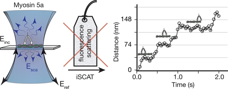
Optical detection of individual proteins requires fluorescent labeling. Cavity and plasmonic methodologies enhance single molecule signatures in the absence of any labels but have struggled to demonstrate routine and quantitative single protein detection. Here, we used interferometric scattering microscopy not only to detect but also to image and nanometrically track the motion of single myosin 5a heavy meromyosin molecules without the use of labels or any nanoscopic amplification. Together with the simple experimental arrangement, an intrinsic independence from strong electronic transition dipoles and a detection limit of <60 kDa, our approach paves the way toward nonresonant, label-free sensing and imaging of nanoscopic objects down to the single protein level.
Keywords: Single molecule detection, label-free, biosensing, myosin 5a, interferometric scattering microscopy
Single molecule optics has contributed considerably to our understanding of a broad range of fundamental processes in physics, chemistry, and biology. Following the first optical detection of single molecules by absorption,1 all subsequent methodologies relied on the observation of fluorescence emission to differentiate the species of interest from an otherwise overwhelming background.2 Despite its many advantages, fluorescence labeling has a number of drawbacks such as limited observation periods due to photobleaching and blinking3 and artifacts induced by the orientation of the transition dipoles.4 Most importantly, chemical or genetic labeling is necessary to visualize single molecules since most biological species are nonfluorescent.
As a consequence, many attempts have been made to find all-optical single molecule alternatives to fluorescence detection. Surface-enhanced Raman spectroscopy exhibits remarkable sensitivity and even chemical specificity,5 but requires nanometer-precise positioning of the analyte close to atomically rough and difficult to control metallic structures. Approaches based on extinction,6 stimulated emission,7 and photothermal8 detection have recently demonstrated single molecule sensitivity even for nonfluorescent molecules. All these techniques, however, require sophisticated noise or background suppression methodologies and strong electronic transition dipoles at the optical detection wavelength.
Nonresonant detection at the single protein level has been thought to require amplification of the weak optical signature from a single molecule. Cavity and plasmonic sensors have reported single molecule sensitivity9−11 but require complex experimental setups and are subject to large variations in the single molecule signals, making quantitative studies difficult. In addition, imaging and studying dynamics on the nanoscale are unachievable by design as it is difficult to obtain spatial information because movement of the analyte does not result in a spatially distinct signal. Here, we show that interferometric scattering microscopy (iSCAT)12−14 can detect, image, and track the motion of individual proteins without the need for any labels in biologically compatible conditions, demonstrated here with the molecular motor, myosin 5a heavy meromyosin (HMM).
Interferometric scattering microscopy relies on the detection of scattered light from the sample in an optical microscope.12,13 Imaging is performed in a reflective geometry, similar to well established approaches such as interference reflection microscopy15,16 or reflection interference contrast microscopy17 but with higher sensitivity achieved through the use of coherent light sources and optimized detection methodologies.18 The area illuminated through the imaging objective consists of a sparse sample of weak scatterers placed at the focus, which allows most of the incident light to pass through the sample (Figure 1A). The glass/water interface reflects 0.5% of the incident light, which is collected by the objective together with a fraction of any scattered light from the sample. The expression for the light intensity, Idet, impinging on a detector that collects scattered and reflected light is given by
| 1 |
where Er, Es, and Ei are the reflected, scattered, and incident electric field amplitudes, s is the scattering amplitude, r is the reflectivity of the interface, and ϕ is the combination of scattering phase and the phase of the reflected light field.19 For small scatterers, |s|2 rapidly approaches zero and only the interference term, 2r|s|sinϕ, remains.
Figure 1.
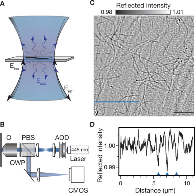
Interferometric scattering microscopy of biomolecules. (A) Schematic of the sample region including incident Einc, reflected Eref, and scattered Esca light fields. (B) Experimental setup. O, objective; QWP, quarter wave plate; PBS, polarizing beamsplitter; AOD, acousto-optic deflector. (C) iSCAT image of individual, unlabeled actin filaments adhered to a microscope cover glass. Pixel nonuniformity and illumination inhomogeneity is removed by flat-fielding with a temporal median filter (see Methods). Scale bar: 5 μm (black line). (D) Signal profile of the blue line in (C) shows three actin filaments indicated by the blue arrowheads.
The corresponding experimental setup is similar to a standard confocal scanning microscope with the exception that the reflected and scattered photons are extracted efficiently by combining a quarter wave plate with a polarizing beamsplitter rather than being rejected by a fluorescence filter (Figure 1B). In addition, the collected light is not passed through a pinhole but is instead imaged onto a CMOS camera. Rapid scanning of the incident beam by acousto-optical deflectors at a rate much faster than the exposure time of the camera achieves uniform illumination of the sample. Using a loosely focused beam in this illumination scheme significantly reduces interference fringes caused by multiple reflections inside the objective compared to standard wide-field illumination.13 The final image produced consists of small features on top of a large background.
The high sensitivity of iSCAT makes it possible to visualize very weak scatterers without the use of any labels. As an example, individual actin filaments bound to a microscope cover glass are readily observed (Figure 1C). In addition to the filaments, the nanometer roughness of the cover glass generates a static background that appears as noise but is reproducible in consecutive acquisitions. The cross section in Figure 1D illustrates the relative magnitudes of the filaments and surface roughness signals. While filaments generate a signal on the order of 1.0%, the background fluctuations of 0.3% ensure that the filaments remain faintly visible above the background. The magnitude of the iSCAT signal for individual actin filaments can be understood by considering its linear dependence on the polarizability and thus molecular weight of the scatterer. Within a diffraction limited spot (200 nm) containing a portion of an actin filament, there are about 75 actin subunits of total molecular mass 3.1 MDa. A SV40 virus-like particle with a molecular mass of 15 MDa produces an iSCAT contrast of 4.5% in our current experimental arrangement,13 resulting in an expected actin iSCAT contrast of 0.9%, in excellent agreement with our experimental observations (Figure 1D).
The linear dependence of the scattering signal on the number of protein molecules in the focus of the microscope poses the question whether individual proteins can be detected with iSCAT. We chose a recombinant heavy meromyosin (HMM)-like fragment of the molecular motor myosin 5a as a test case because it has been very well characterized as a processive actin-dependent motor and its processive properties are a robust indicator of single molecule detection.20 We introduced GFP at the C-terminus of myosin 5a HMM to enable direct comparison with established single molecule fluorescence-based imaging without having to use separate preparations but emphasized that the small size (40 kDa) and the weak transition dipole at 445 nm of GFP are insufficient to generate an iSCAT signal greater than 0.02%. On the basis of the above calculation and the molecular weight of the myosin 5a construct (502 kDa) the iSCAT contrast for a single myosin 5a HMM molecule is expected to be on the order of 0.15%. Such signals are smaller than those generated both by individual actin filaments and the roughness of the glass making it difficult to observe myosin directly in images such as that shown in Figure 1C. However, upon addition of ATP myosin 5a HMM moves along actin filaments while all other features of the iSCAT image remain stationary. Therefore, subtraction of an image containing all stationary iSCAT features from the original frames, which we term differential imaging, will reveal changes in sample scattering due to mobile objects in this case myosin 5a.
Under ideal conditions, the only noise source that could overwhelm the signal originating from weak scatterers for differential imaging are fluctuations in the background level caused by shot noise in the detection of photoelectrons by the imaging system. Commercially available digital cameras usually saturate at 104–105 photoelectrons per pixel resulting in a baseline noise on the order of 0.3% root-mean-squared (RMS) in the best case for individual images (Figure 2A).
Figure 2.

Interferometric scattering detection of myosin 5a HMM at the single molecule level. (A) Sequence containing M iSCAT images, xi, of actin filaments on a microscope cover glass in the presence of myosin 5a HMM. Camera exposure time set at 0.40 ms with a frame time of 0.58 ms, [ATP] = 5 μM. (B) An image containing purely stationary iSCAT features obtained by taking the median or averaging over the sequence of images in (A). (C) Sequence of M differential iSCAT images, yi, obtained by subtracting the stationary iSCAT features from the image sequence in (A). (D) Time-averaged differential images generated by binning N = 170 consecutive frames together. Note the order of magnitude decrease in z-scale from (C) to (D). Scale bars: 1 μm (black line).
Given that the background is constant, we can generate a low-noise image of the static iSCAT background consisting largely of actin filaments and the glass substrate by replacing each pixel with the median value from a sequence of images or averaging together several frames (Figure 2B). After subtraction of the static background from each individual image, the differential images show signals due to mobile iSCAT features and shot noise (Figure 2C), which can be reduced further by summing consecutive images and thus accumulating more photoelectrons. We remark that the background image does not need to be acquired either in the absence of myosin 5a or ATP as computing the median intrinsically removes any nonstationary contributions that occur either as a consequence of binding/unbinding of myosin 5a or movement in the presence of ATP (see Methods section). Our camera allowed detection of an 104 × 104 pixel2 area at a frame rate of 1.7 kHz. Time-averaging consecutive differential frames to a bandwidth of 10 Hz increases the electron count per pixel to 2 × 10⁷ and thus reduces the baseline fluctuations to 0.024%. Upon averaging 170 differential images, we observed several diffraction-limited spots that coincide spatially with the actin filaments in the presence of ATP (Figure 2D and Supporting Information Movie S1). The specific binding to actin together with the processive motion along these filaments, suggests that these features are due to myosin 5a HMM molecules. Importantly, myosin molecules become visible above the background because they are the only mobile component of the sample and are thus not removed by the subtraction of the median image generated from the image stack.
The dramatic effect of time averaging on the visibility of small iSCAT signals is illustrated by plotting image cross sections as a function of averaged images (Figure 3A). For individual image subtraction, the standard deviation amounts to 0.3% as expected from the well depth of the imaging camera. As the number of averaged images increases, however, the shot noise drops to the point where an iSCAT signal of the order of 0.2% becomes clearly visible. The evolution of the standard deviation of the background as a function of the number of averaged images shows shot noise-induced behavior down to the 60 kDa level (Figure 3B). At this point, the achievable baseline fluctuations begin to deviate from shot noise due to the introduction of other noise sources that affect the differential images, which in our case amounts to mechanical drift (<10 nm ) of the sample position and to small fluctuations in laser intensity.
Figure 3.

iSCAT as an all-optical single protein sensor. (A) One-dimensional cut across a single differential myosin 5a HMM iSCAT signal for integration times ranging from 0.58 to 348.00 ms. The signal in (A) is assigned to be a single myosin 5a HMM molecule due to its processive nature, characteristic 37 nm steps, and contrast value of 0.18%. The cross section was chosen along the x-axis with no particular orientation relative to the underlying actin filament whose iSCAT signal is removed by the differential imaging scheme. (B) Background noise as a function of the number of averaged images. Solid line indicates shot noise behavior. We added a second vertical axis corresponding to the molecular weight detectable at a signal-to-noise ratio of 1 as a function of integration time. In the case of myosin 5a, this number corresponds to 1 ms. The dashed gray line represents the molecular weight of myosin 5a HMM. The detection limit thus corresponds to 60 kDa at an integration time of 300 ms in the current experimental arrangement.
Although specific binding and motion along actin filaments strongly suggest the observation of individual myosin 5a HMM molecules, further proof requires comparison with established fluorescence21 or optical tweezer22 based single-molecule assays. The distributions of velocity (Figure 4A), run lengths at saturating ATP concentrations (1 mM) (Figure 4B) and the velocity dependence on ATP concentration (Figure 4C) all show excellent agreement with previous single molecule studies.21−24 In addition, we evaluated the iSCAT contrast for 249 different molecules from several tens of image stacks analyzed as shown in Figure 2. We obtained a single distribution with an iSCAT contrast centered around 0.18% in good agreement with our theoretical prediction of the iSCAT contrast for a single myosin 5a molecule (Figure 4D). The spread of contrasts is likely due to small variations in focusing, the lack of control over the orientation of the protein relative to the incident polarization and possible displacements of the protein relative to the substrate. For scatterers with a contrast of 0.3%, the localization accuracy was on the order of 5 nm and thus sufficient to observe distinct, 37 nm steps as expected for myosin 5a (Figure 4E).
Figure 4.

Myosin 5a HMM processivity characterized by iSCAT at the single molecule level. (A,B) Velocity and processivity at saturating ATP concentrations (1 mM, n = 91). (C) Velocity as a function of ATP concentration. The solid curve represents the best fit of the velocity data to the relationship V = ds/(1/k1[ATP] + 1/k2), where ds represents the average step size assumed to be 37 nm, k1 is the second order ATP binding rate constant, and k2 is the first order ADP release rate constant. (D) Histogram of iSCAT contrasts obtained from finding the center of mass of 249 separate processive molecules. All visible processive signatures from 15 recordings were included in the histogram and no additional preselection was performed. Data was originally recorded at 1.7 kHz and then 170 consecutive frames were averaged together for this analysis. (E) Distance traveled for a single myosin 5a molecule with contrast of 0.31% at 10 μM ATP concentration. Imaging speed: 1 kHz averaged to 25 Hz (see Supporting Information Movie S4). (F) Sample quality assessment of myosin 5a HMM used in this study by electron microscopy. Upper panel shows an electron micrograph of the construct, scale bar: 50 nm. Lower panels show examples of individual myosin 5a HMM molecules at higher magnification, scale bar: 20 nm. The sample was confirmed to be without aggregates and dimeric with bound light chains.
The above observations and the excellent match between expected and observed iSCAT contrast for a single myosin 5a HMM molecule together with the following arguments strongly suggest that the observed moving objects are single myosin 5a molecules and not aggregates or other species. The same preparation of myosin 5a HMM investigated by negative staining electron microscopy under similar concentrations and ionic strengths as used in the single molecule motility experiments showed a very homogeneous distribution of objects consisting predominantly of double-headed myosin molecules with a coiled-coil tail and with no larger aggregates that could lead to exaggerated iSCAT signal (Figure 4F).25 The movement of objects was very robust, which is inconsistent with aggregates given the negligible amount of aggregation observed in the preparation (Supporting Information Movie S1). These conclusions are further supported by single molecule fluorescence assays performed with the same preparation of myosin 5a HMM by detecting the fluorescence of the GFP fusion moiety. We observed very similar amounts of both bound and transiently binding molecules in iSCAT and fluorescence measurements performed on the same sample consecutively on different instruments (Supporting Information Movies S2, S3). Simultaneous iSCAT and fluorescence, although in principle possible,13 was difficult to achieve here due to the rapid photobleaching of GFP by the iSCAT illumination beam at 445 nm.
Label-free detection does not allow for the observation of signatures such as photoblinking, bleaching, or antibunching of the emission that act as proof for the observation of single molecules. We thus chose myosin 5a HMM because its processive properties have become generally accepted as a signature for the presence of single molecules through a variety of optical experiments.21−24 In addition, the observation of specific binding to actin (Supporting Information Movies S1, S2) mimics the operation of any sensor, that is, the comparison of a signal in the presence and absence of the analyte. In cavity-based techniques,9 the signal is the resonance frequency, while for plasmonic sensors it is the maximum of the plasmon resonance.10,11 In iSCAT, the signal is the surface scattering in the absence or presence of a single protein.
iSCAT has three important advantages over all currently available approaches to label-free single molecule sensing. Firstly, single molecule signals show a single distribution about a maximum signal that is directly proportional to the mass of the analyte (Figure 4D). This is in contrast to current optical technologies capable of detecting single molecules without labels, such as plasmonic and cavity-based sensors whose signals fluctuate between zero and a maximum signal, making quantification much more difficult. Secondly, iSCAT provides spatial information that is useful in combination with patterned surfaces often used in sensing applications and enables direct comparison of affinities in a single measurement. Finally, the experimental setup is comparatively simple, requiring only an inverted microscope and a glass coverslip as the sensor.
Our results disprove the notion that the scattering cross sections of single proteins are orders of magnitude too small to be detected in an optical microscope. Even complex spectroscopic investigations now routinely operate with sensitivities at the 10–5 level or below26 at which detection and imaging of small proteins on the order of 60 kDa would still occur at excellent SNRs of 10 with iSCAT. Critically, however, the presented detection modality does not require any specific molecular properties, such as strong transition dipoles, nor does it depend on sophisticated methodologies to reduce laser intensity noise or nanoscopic amplification of the weak single molecule signal. Instead, the imaging camera performs noise reduction automatically through the accumulation of detected photoelectrons with time and no specific refractive index environments are necessary. Together with the possibility of combining iSCAT with single molecule fluorescence13 and the potential for unlimited observation times due to a lack of photobleaching our results enable novel applications from biosensing to multidimensional tracking of single biomolecules.
Materials and Methods
Experimental Setup
The experimental setup is similar to that described in ref (13). Briefly, the output of a 445 nm diode laser is spatially filtered and adjusted to 2 mm beam diameter before passing through two acousto-optic deflectors (AOD, Gooch and Housego). The beam deflections generated by the AODs are imaged with telecentric lenses into the back focal plane of an oil immersion objective (Olympus PLAPON 1.42 NA, 60×) after passing through a polarizing beam splitter (PBS). The small beam diameter underfills the back aperture of the objective to generate a focal spot of ∼1 μm full width at half-maximum (fwhm). A quarter wave plate before the objective causes any reflected and scattered light by the sample to get reflected by the PBS before being imaged onto a CMOS camera (Photonfocus MV-D1024-160-CL-8) at either 167× or 333× magnification by choosing the appropriate focal length imaging lens. The incident power is adjusted to achieve near-saturation of the CMOS camera amounting to 2.5 and 10 kW/cm2 at the sample at 1.0 ms exposure time for the two magnifications.
The two AOD channels are scanned in a sawtooth fashion by separate, phase-locked function generators at 84 and 83 kHz, respectively. Both the absolute and relative frequencies are chosen to induce the smallest detectable fluctuations in the background light intensity on the time scale of the camera exposure time. Even though the frequency difference (1 kHz) nominally suggests a minimum exposure time of 1 ms, this requirement is relaxed by the large spot size. For a fwhm of 1 μm, few tens of scans over an area of 10 × 10 μm2 are sufficient to generate a highly uniform illumination. At the given scan speeds, this process only takes ∼100 μs, much faster than the shortest exposure time. Any spot broadening induced by the limited speed of the acoustic wave in the deflector only serves to further smoothen the illumination. Rapid scanning and illumination of an area four times larger than what is imaged by the camera avoids the introduction of diffraction fringes from the edges of the sawtooth pattern and eventually allows for shot noise limited sensitivity toward the 10–4 level.
Data Recording and Analysis
To produce images such as Figure 1C it is necessary to remove any constant background caused by residual reflections and illumination inhomogeneities. To do so we record 100 images while manually moving the sample stage and then replace each pixel by the temporal median value of the frame sequence to generate an optimal flat field image that is independent of the sample. After division by the flat field image, we obtain sample-specific images with shot noise limited sensitivity, which simplifies the initial alignment and choosing an appropriate region. Finding the correct focal point is critical and can be estimated by maximizing the contrast from individual actin filaments, although fine adjustment during the recording is necessary. The latter is achieved by recording a single image and subtracting it from the live preview that only reveals changes in the sample scattering compared to the original background image. In the presence of myosin 5a HMM, such a subtraction leads to differential images such as those shown in Supporting Information Movie S3. To reduce the effects of sample drift along the optical axis, we stabilize the focus by monitoring the back-reflection of a totally internal reflected beam at 633 nm.
To generate an image containing all the static iSCAT features we performed a temporal median filter over the range of images in which the myosin 5a HMM molecule was processive, typically greater than 1000 frames. Alternatively, consecutive frames that lacked myosin 5a HMM signals were averaged together to produce the static iSCAT background image. Contrast values for single myosin 5a HMM were determined by the pixel value corresponding to the center of mass of the point spread function.
For myosin 5a detection, we initially used 166× magnification, 104 × 104 pixel2 field of view at 63.6 nm/pixel, a frame rate of 1.7 kHz and time averaged the differential images to 10 Hz. For tracking, we increased the magnification to 333× with a 128 × 128 pixel2 field of view and a frame rate of 1.0 kHz to improve the electron count and therefore the signal-to-noise ratio. Nanometric tracking was performed by time averaging the differential images to 25 Hz and then fitting the point spread function to a two-dimensional Gaussian.
Interferometric Scattering Microscopy Sample Preparation
Rabbit skeletal muscle actin27 and mouse myosin 5a HMM28 with a C-terminal GFP were prepared as described and stored in liquid nitrogen until used. A 20 μM actin stock solution was prepared in polymerization buffer (10 mM imidazole, 50 mM KCl, 1 mM MgCl2, 1 mM EGTA, pH 7.3 containing 1.7 mM DTT, 3 mM ATP). Actin was diluted to 200 nM in motility buffer (MB; 20 mM MOPS pH 7.3, 5 mM MgCl2, 0.1 mM EGTA).
Borosilicate cover glasses (No. 1.5, 24 × 50 mm, VWR) were cleaned by sequential rinsing with Milli-Q water, ethanol, and water. They were then dried under a stream of dry nitrogen and exposed to UV/ozone for 8 min at 50 W power using a plasma cleaner (Diener Electronic, Plasma System Femto). All cover glass was used within one day of cleaning. A single flow cell was then assembled using double-sided transparent tape (Scotch) and a second cover glass (No. 1, 24 × 40 mm, VWR).
The flow cell was rinsed with 1 mg/mL solution of poly(ethylene glycol)-poly l-lysine (PEG-PLL) branch copolymer (Surface Solutions SuSoS, Switzerland) in phosphate buffered saline and incubated for 30 min. Next, it was washed twice with MB and actin solution was added. After 5 min of incubation, the chamber was washed with MB and the surface was blocked by adding 1 mg/mL BSA in MB and subsequent incubation for 5 min. A solution of 2–10 nM myosin (MB containing 40 mM KCl, 5 mM DTT, 0.1 mg/mL BSA, and 5 μM calmodulin) was added, incubated for 5 min, and then washed. Upon addition of ATP, myosin movement was observed.
Electron Microscope Sample Preparation
Myosin 5a HMM was diluted to 50 nM in buffer containing 10 mM MOPS (pH 7.0), 2 mM MgCl2, 0.1 mM EGTA, and 40 mM KCl. A 5 μL drop of sample was applied to a carbon-coated copper grid (pretreated with UV light) and stained with 1% uranyl acetate. Micrographs were recorded at 60 000× on a JEOL 1200EX II microscope. Data were recorded on an AMT XR-60 CCD camera. Catalase crystals were used as a size calibration standard.
Acknowledgments
P.K. is supported by the John Fell Fund, a career acceleration fellowship by the EPSRC (EP/H003541) and an ERC starting grant (NanoScope). K.S. was supported by a fellowship from the National Institute of Biomedical Imaging and Bioengineering, National Institutes of Health (FEB013960). J.O.A was supported by a scholarship from CONACyT to pursue his doctoral work (scholar: 213546). J.A. was supported by a Marie Curie Fellowship (330215). J.R.S. was supported by the intramural funds from the National Heart, Lung, and Blood Institute, National Institutes of Health (ZIA HL004229). The authors thank the Electron Microscopy Core Facility of the NHLBI for support and the use of facilities.
Supporting Information Available
Supporting movies S1–S4. This material is available free of charge via the Internet at http://pubs.acs.org.
Author Present Address
(K.M.S.) MRC National Institute for Medical Research, The Ridgeway Mill Hill, London, NW7 1AA, U.K.
The authors declare no competing financial interest.
Direct detection of single proteins as small as 60 kDa and imaging of 340 kDa proteins with 5 nm localization precision was recently demonstrated in a bio-sensing assay with iSCAT using a slightly different illumination scheme.29 The reported iSCAT contrast for a 340 kDa protein of 0.1% agrees well with the linear relationship between iSCAT contrast and molecular weight reported in this work.
Funding Statement
National Institutes of Health, United States
Supplementary Material
References
- Moerner W. E.; Kador L. Phys. Rev. Lett. 1989, 62, 2535–2538. [DOI] [PubMed] [Google Scholar]
- Orrit M.; Bernard J. Phys. Rev. Lett. 1990, 65, 2716–2719. [DOI] [PubMed] [Google Scholar]
- Dickson R. M.; Cubitt A. B.; Tsien R. Y.; Moerner W. E. Nature 1997, 388, 355–358. [DOI] [PubMed] [Google Scholar]
- Enderlein J.; Toprak E.; Selvin P. R. Opt. Express 2006, 14, 8111–8120. [DOI] [PubMed] [Google Scholar]
- Nie S.; Emory S. R. Science 1997, 275, 1102–1106. [DOI] [PubMed] [Google Scholar]
- Kukura P.; Celebrano M.; Renn A.; Sandoghdar V. J. Phys. Chem. Lett. 2010, 1, 3323–3327. [Google Scholar]
- Chong S.; Min W.; Xie X. S. J. Phys. Chem. Lett. 2010, 1, 3316–3322. [Google Scholar]
- Gaiduk A.; Yorulmaz M.; Ruijgrok P. V.; Orrit M. Science 2010, 330, 353–356. [DOI] [PubMed] [Google Scholar]
- Armani A. M.; Kulkarni R. P.; Fraser S. E.; Flagan R. C.; Vahala K. J. Science 2007, 317, 783–787. [DOI] [PubMed] [Google Scholar]
- Ament I.; Prasad J.; Henkel A.; Schmachtel S.; Sönnichsen C. Nano Lett. 2012, 12, 1092–1095. [DOI] [PubMed] [Google Scholar]
- Zijlstra P.; Paulo P. M. R.; Orrit M. Nat. Nanotechnol. 2012, 7, 379–382. [DOI] [PubMed] [Google Scholar]
- Lindfors K.; Kalkbrenner T.; Stoller P.; Sandoghdar V. Phys. Rev. Lett. 2004, 93, 037401. [DOI] [PubMed] [Google Scholar]
- Kukura P.; Ewers H.; Müller C.; Renn A.; Helenius A.; Sandoghdar V. Nat. Methods 2009, 6, 923–927. [DOI] [PubMed] [Google Scholar]
- Ortega Arroyo J.; Kukura P. Phys. Chem. Chem. Phys. 2012, 14, 15625. [DOI] [PubMed] [Google Scholar]
- Vašíček A. Opt. Spectrosc. 1961, 11, 128. [Google Scholar]
- Curtis A. J. Cell Biol. 1964, 20, 199–215. [DOI] [PMC free article] [PubMed] [Google Scholar]
- Zilker A.; Engelhardt H.; Sackmann E. J. Phys. (Paris) 1987, 48, 2139–2151. [Google Scholar]
- Celebrano M.; Kukura P.; Renn A.; Sandoghdar V. Nat. Photonics 2011, 5, 95–98. [Google Scholar]
- Kukura P.; Celebrano M.; Renn A.; Sandoghdar V. Nano Lett. 2009, 9, 926–929. [DOI] [PubMed] [Google Scholar]
- Sellers J. R.; Veigel C. Curr. Opin. Cell Biol. 2006, 18, 68–73. [DOI] [PubMed] [Google Scholar]
- Yildiz A.; Forkey J. N.; McKinney S. A.; Ha T.; Goldman Y. E.; Selvin P. R. Science 2003, 300, 2061–2065. [DOI] [PubMed] [Google Scholar]
- Rief M.; Rock R. S.; Mehta A. D.; Mooseker M. S.; Cheney R. E.; Spudich J. A. Proc. Natl. Acad. Sci. U.S.A. 2000, 97, 9482–9486. [DOI] [PMC free article] [PubMed] [Google Scholar]
- Snyder G. E.; Sakamoto T.; Hammer J. A. III; Sellers J. R.; Selvin P. R. Biophys. J. 2004, 87, 1776–1783. [DOI] [PMC free article] [PubMed] [Google Scholar]
- Baker J. E.; Krementsova E. B.; Kennedy G. G.; Armstrong A.; Trybus K. M.; Warshaw D. M. Proc. Natl. Acad. Sci. U.S.A. 2004, 101, 5542–5546. [DOI] [PMC free article] [PubMed] [Google Scholar]
- Walker M. L.; Burgess S. A.; Sellers J. R.; Wang F.; Hammer J. A.; Trinick J.; Knight P. J. Nature 2000, 405, 804–807. [DOI] [PubMed] [Google Scholar]
- Dobryakov A. L.; Kovalenko S. A.; Weigel A.; Pérez-Lustres J. L.; Lange J.; Müller A.; Ernsting N. P. Rev. Sci. Instrum. 2010, 81, 113106. [DOI] [PubMed] [Google Scholar]
- Spudich J. A.; Watt S. J. Biol. Chem. 1971, 246, 4866–4871. [PubMed] [Google Scholar]
- Wang F.; Chen L.; Arcucci O.; Harvey E. V.; Bowers B.; Xu Y.; Hammer J. A.; Sellers J. R. J. Biol. Chem. 2000, 275, 4329–4335. [DOI] [PubMed] [Google Scholar]
- Piliarik M.; Sandoghdar V. arXiv:1310.7460v2, 2013.
Associated Data
This section collects any data citations, data availability statements, or supplementary materials included in this article.