Micro-heterogeneity metrics for diffusion in soft matter

Abstract

Passive particle tracking of diffusive paths in soft matter, coupled with analysis of the path data, is firmly established as a fundamental methodology for characterization of both diffusive transport properties (the focus here) and linear viscoelasticity. For either focus, particle time series are typically analyzed by ensemble averaging over paths, a perfectly natural protocol for homogeneous materials or for applications where mean properties are sufficient. Many biological materials, however, are heterogeneous over length scales above the probe diameter, and the implications of heterogeneity for biologically relevant transport properties (e.g. diffusive passage times through a complex fluid layer) motivate this paper. Our goals are three-fold: first, to detect heterogeneity as reflected by the ensemble path data; second, to further decompose the ensemble of particle paths into statistically distinct clusters; and third, to fit the path data in each cluster to a model for the underlying stochastic process. After reviewing current best practices for detection and assessment of heterogeneity in diffusive processes, we introduce our strategy toward the first two goals with methods from the statistics and machine learning literature that have not found application thus far to passive particle tracking data. We apply an analysis based solely on the path data that detects heterogeneity and yields a decomposition of particle paths into statistically distinct clusters. After these two goals are achieved, one can then pursue model-fitting. We illustrate these heterogeneity metrics on diverse datasets: for numerically generated and experimental particle paths, with tunable and unknown heterogeneity, on numerical models for simple diffusion and anomalous sub-diffusion, and experimentally on sucrose, hyaluronic acid, agarose, and human lung culture mucus solutions.

1 Introduction

Soft materials, especially biological ones, are often heterogeneous on microscopic to macroscopic length scales. In some cases, this heterogeneity is inherent, like the different “compartments” inside of a living cell¹. In other cases it reflects a material’s multi-functionality; for instance, a heterogeneous mesh-size distribution in mucus barrier layers² from lung airways may endow the material with the ability to simultaneously regulate and differentiate diffusive transport of a wide range of inhaled particle sizes. Likewise, such a heterogeneous mesh distribution may endow the material with the ability to tune viscoelastic moduli across a wide frequency spectrum. In response to disease conditions, biological materials such as pulmonary mucus become modified, ^3–5 with consequences for both diffusive and viscoelastic properties,⁶ and their degree of heterogeneity is likewise expected to change. It would be valuable to have practical tools to detect and quantify material heterogeneity, and to discern modifications in these features as a result of disease and disease progression. Our interest in this paper is in the development of quantitative metrics for diffusive heterogeneity of soft matter at the micron to sub-micron scale accessible by standard microscopy and particle tracking techniques. We illustrate these tools on numerically generated data for normal diffusive and sub-diffusive stochastic processes, and on experimental data for four diverse fluids: sucrose, hyaluronic acid, agarose, and mucus.

Microrheology^7–9 has emerged as a powerful experimental tool for transport property characterization of soft biological materials at the microscale. For a discussion of experimental techniques encompassed by microrheology we point the reader to the review article by Waigh⁷. A class of microrheology methods, based on the analysis of thermal motion of embedded particles, is known as passive particle tracking microrheology (PPTM). This technique uses video microscopy to track the position time series of passive tracer particles to estimate the viscous and elastic moduli of the medium.¹⁰ Traditionally, characterization of the sample material is based on ensemble averaging of the path data. For a homogeneous system, where all the beads experience the same environment, the distribution of increments (displacements between observations of bead position) sampled by the ensemble arise from the same stochastic process and the ensemble data is expected to fit to a single Gaussian curve. Material parameters are then inferred from the variance of the fitted Gaussian; e.g., the diffusion coefficient for simple Brownian motion in viscous fluids. In materials that exhibit micro-heterogeneity, different particles probe different environments, and although the step-size distributions of individual paths are described by Gaussians, the distribution of displacements across multiple paths will be non-Gaussian. Accordingly, the presence of heterogeneity is captured by deviations from Gaussian behavior. Several standard tests of Gaussianity are cited below from the PPTM literature. In the following sections we present methods from the statistics and machine learning literature that simultaneously detect heterogeneity and divide the path data into clusters of statistically indistinguishable paths.

Finally, we are interested in predictive consequences of heterogeneity beyond the timescales of the experimental observations, which requires a final model fitting step. In the best case scenario, there are rigorous theoretical models derived from detailed molecular-scale knowledge of the physical and chemical properties of the soft matter system and the interaction of the embedded probes with the molecular structure. In such a scenario, one has candidate models to choose from, and model selection methods can be applied^11,12 to yield a best-fit model. The classical example is simple Brownian motion for diffusion in a viscous fluid, where there is a unique model and model parameters.

For soft matter systems, which, unlike simple viscous fluids, possess viscoelastic relaxation modes and thereby memory in the diffusive path data, there are very few systems for which a rigorous diffusive transport theory has been derived from first principles. The list shortens if one requires that the MSD scaling behavior and other statistical properties are exactly solvable. The rare model systems with these criteria are celebrated, including the Rouse model for dilute, monodisperse polymer melts, and the Zimm model which couples solvent hydrodynamic interactions to the Rouse model. The reader is referred to the monograph of Rubinstein and Colby¹³ and the work of Cai et al.¹⁴ for a detailed discussion, including additional scaling behavior associated with models for semidilute and entangled polymers. These first-principles models yield anomalous, sub-diffusive, mean-squared displacement (MSD) scaling behavior with exponents 1/2 or 2/3 on intermediate timescales, followed by convergence to simple diffusion and MSD exponent 1 for sufficiently long timescales.

Complex fluids in biology are typically mixtures of molecular species of diverse molecular weights, and with attractive and repulsive interactions between them. Electrostatic interactions between the probe and soft matter sample, likewise, can significantly alter particle diffusion (cf. MacKintosh¹⁵). This observation has been extensively explored for drug particle delivery through mucus barriers in the lung.² For such biological soft matter systems, there is no rigorous theory to guide model selection beyond the ideal systems noted above, whereas PPTM data in biological fluids such as pulmonary mucus (cf. Hill et al.⁶) yields MSD exponents that span the entire interval (0,1].

Thus, until such time that a rigorous theory exists of diffusive properties of complex biological fluids and the effects of probe-fluid interactions, even for homogeneous complex fluids, the analysis of the particle path data must be performed by statistical methods with minimal assumptions of the underlying models to discern among different fluids and different particles in a given fluid. That is the perspective taken in this paper in regard to the first two goals of heterogeneity detection among the ensemble of paths and clustering of the paths.

There are, nonetheless, ad hoc stochastic models that share several key features of the PPTM data in biological and biomimetic fluids. These include fractional Brownian motion (cf. Kou and coworkers¹⁶) and generalized Langevin equations with special memory kernels (cf. Mason and Weitz¹⁰, colloidal diffusion^17,18, McKinley et al.¹⁹). The proper statistical approach, given a candidate list of potential models, is to rank the likelihood that the observed data arises from each candidate model. A rigorous protocol for model selection is beyond the scope of this paper, and will be presented elsewhere.¹²

Here, we will review the current best practices in PPTM, both at the level of detection of statistically significant heterogeneity (without reference to a particular model) and at the level of models and parameter fitting. We emphasize that the techniques of data analysis discussed in this paper are novel only in their application to PPTM data. Thus we do not provide an historical review of these statistical techniques, and refer the reader instead to standard publications^20–23.

Many research teams have used PPTM data analysis to infer a degree of heterogeneity in soft biological materials ^24–33. These efforts include two broad categories: one based on the “Gaussianity” of the distribution of particle displacements and the second on the statistics of the individual particle mean-squared-displacements (iMSD). We propose a new protocol that combines standard Machine Learning techniques, such as the Expectation Maximization algorithm³⁴ and hierarchical clustering³⁵, to identify statistically distinct clusters based on the distribution of particle path statistics, without reference to the stochastic processes that generated the paths. In using these techniques, we rely upon two relatively weak assumptions: that each path has Gaussian increments, and, that the process generating each path is stationary. The resulting semiparametric protocol is consistent both with a large number of stochastic processes and with current approaches to heterogeneity detection in the literature.

Once the particle paths have been assigned to statistically distinct clusters, we then consider the inverse problem of fitting the ensemble of paths in each cluster to models for simple diffusive and anomalous sub-diffusive processes. Unlike simple diffusion where the mean squared displacement (MSD) grows linearly in lagtime (τ), anomalous subdiffusion is described by a power law, MSD ∼ τ^α, with 0 < α < 1. Anomalous subdiffusion has been found in many biological contexts; diffusion of 1-micron diameter particles in HBE mucus,⁶ diffusion of biopolymers inside cells,³⁶ bacteria chromosomal loci,³⁷ movement of lipids on model membranes,³⁸ proteins diffusion in organellar membranes³⁹ and in the nucleoplasm.⁴⁰ Model fitting of each cluster to candidate models for the underlying stochastic process affords predictive power for elusive experimental properties such as passage times, as illustrated in Hill et al.,⁶ and addressed in detail in Lysy et al.¹²

In the next section, we start by summarizing existing metrics for the detection and assessment of heterogeneity in PPTM. In Section 4 we describe our metrics that have precedent in the statistics and machine learning literature and compare them with best practices on numerically generated data. In Section 5 we apply our metrics to numerically generated and experimental data, beginning with systems where the heterogeneity is controlled in order to illustrate the precision of our tools. We close with application of these metrics to particle data in an agarose solution, an oft-used simulant for biological gels that is typically non-homogeneous, and finally to particle data in human bronchial epithelial cell culture mucus. In these last two experiments, the degree of heterogeneity is not known a priori, representing the typical scenario for application of these tools for PPTM data on a soft matter sample and probe particle of interest.

2 Current metrics to detect heterogeneity in PPTM data

Several groups^{24,28,30–32,41} use the van Hove correlation function, P(Δx(τ)),⁴² which is the probability distribution function constructed from the observed increments or displacements, Δx, at lag time τ, where

$$\mathrm{\Delta }x(\tau )=x(t+\tau )-x(t).$$ (1)

For the majority of relevant stationary, stochastic increment processes that have been used to model PPTM, including normal diffusion, fractional Brownian motion, and generalized Langevin equations, the corresponding van Hove correlation function is Gaussian for each fixed set of model parameters. Paths generated from any of these classical stochastic processes can be considered homogeneous if they arise from the same set of model parameters, or within some small neighborhood of a parameter set. The practical challenge for experimental path data is to develop a test that does not rely on a priori knowledge or assumptions about a model that generated the data. In a heterogeneous environment, identical particles diffuse in regions with different local properties. One may also consider heterogeneity that arises from particles that are polydisperse in some aspect, e.g., diameter (which we will explore below) or surface chemistry.

In the scenario of identical particles in a “sufficiently heterogeneous sample,” a single Gaussian, according to a well-defined statistical metric, fails to fit the ensemble-averaged van Hove correlation function. Heterogeneity can then be measured by the extent to which the van Hove correlation function deviates from a Gaussian form; in other words, one can view the statistical metric as an order parameter measuring departure from Gaussianity. We refer to such metrics as “Stage 1 metrics” and note that they are useful for detection of heterogeneity, but the metric itself is not designed to make predictions beyond the observable data.

Whereas a Stage 1 metric implies the presence of statistically significant heterogeneity, one can proceed to probe further into the underlying heterogeneity by binning the paths into disjoint clusters, which we refer to as a “Stage 2 metric.” We first survey Stage 1 metrics and then address existing Stage 2 metrics. Our approach is a Stage 2 metric that does not require a preliminary Stage 1 step.

2.1 Stage 1 metrics for detection of heterogeneity in PPTM

• Rahman⁴³ proposed a non-Gaussianity parameter NG_τ, which measures the departure from an exact identity satisfied by the second and fourth moments of a Gaussian distribution. Namely, one takes these moments of the van Hove correlation function, and constructs the metric NG_τ defined for each lag time τ by,

  $${\mathit{\text{NG}}}_{\tau }=\frac{\langle \mathrm{\Delta }{x}^4(\tau )\rangle }{3{\langle \mathrm{\Delta }{x}^2(\tau )\rangle }^2}-1.$$ (2)

  If the increments are Gaussian, NG_τ = 0 for every lag time τ, whereas non-zero values of NG_τ denote a degree of heterogeneity. This parameter was later applied to the analysis of colloidal systems by Kegel and van Blaaderen.³¹
• In the PPTM literature, Houghton et al.³² used the excess kurtosis (ku) of the van Hove function, defined as

  $$\mathit{\text{ku}}=\frac{{{\mathrm{\sum }}_{i=1}^n(x_i-\overline{x})}^4}{(n-1){\mathrm{\sigma }}^4}-3,$$ (3)

  to measure heterogeneity. Here x̄ is the mean and σ is the standard deviation of the van Hove correlation function. For a Gaussian distribution ku = 0, and again non-zero values denote a degree of heterogeneity.
• Savin and Doyle⁴⁴ formulated estimators of the square of the ensemble mean squared displacement M₁(τ), and of its corresponding variance, M₂(τ). These estimators are derived from a weighted average of the iMSD where the weights are proportional to the length of the particle trajectory. This prevents the results from being biased by more mobile particles. Rich et al.³⁰ used these estimators to propose a heterogeneity ratio (HR), defined as

  $$\mathit{\text{HR}}=\frac{M_2(\tau )}{M_1{(\tau )}^2}.$$ (4)

  Numerical simulations³⁰ showed that the maximum value of HR for a bimodal fluid is 3. Lower and larger values of HR are then used to quantify heterogeneity, see for example Rich et al.³⁰ and Aufderhorts-Roberts et al.²⁸
• Tseng et al.⁴⁵ employed “bin partitions” of compliance values to determine the degree of heterogeneity. The compliance Γ(τ), is related to the MSD by,⁴⁶

  $$\mathrm{\Gamma }(\tau )=\frac{\pi a}{k_{B}T}\langle \mathrm{\Delta }{r}^2(\tau )\rangle .$$ (5)

  Bin partitions of the compliance distributions were obtained by comparing the relative contributions of the 10%, 25%, and 50% highest values of the individual compliance to the ensemble mean compliance. The relative contributions of these values to the ensemble compliance should be close to 1 for a highly heterogeneous solution and close to 0.1, 0.25, and 0.50, respectively, for a perfectly homogeneous solution.
• Another Stage 1 metric involves the calculation of iMSDs, defined for a particle p as

  $$\mathrm{\Delta }{r}_p^2(\tau )=\frac{1}{N-\tau }{\mathrm{\sum }}_{i=1}^{N-\tau }[{(x_p(t_i+\tau )-x_p(t_i))}^2+{(y_p(t_i+\tau )-y_p(t_i))}^2].$$ (6)

  Duits et al.²⁷ constructed auto- and cross-correlation matrices of the amplitude of iMSD, A_p, to detect both path-wise and temporal heterogeneities. Here the amplitude is found by fitting Eqn. (6) to a power-law function,

  $$\mathrm{\Delta }{r}_p^2(\tau )\cong A_p{\tau }^{\alpha }.$$ (7)

  The authors used normalized variances, both with respect to time and space, to quantify the heterogeneity in the distribution of A_p. We note that this strategy mixes pure path analysis with a presumed model for the scaling of iMSD with lag time τ. It is worthwhile to recognize that the preponderance of passive microrheology applications focuses on the power law exponent α in iMSD, rather than the pre-factor A_p. In future publications, we will address model-fitting methods that justify assumptions such as the iMSD scaling in Eqn. (7), as well as the benefit in fitting both scaling parameters A_p and α to the iMSDs, rather than one or the other.

We highlight one feature of this iMSD strategy that we will adopt in our approach, namely that it is based on cross-correlations among all particle paths, removing any reliance on comparison of the ensemble with one representative path. However, we seek a clustering strategy that does not rely on a model for the underlying particle increment process. We choose to defer any fitting to parametric models after decomposing particle paths into clusters, using only statistics of the raw data to cluster the ensemble. After clustering is complete, we then entertain best-fit models and parameter estimation for each cluster.

2.2 Stage 2 metrics for decomposition of paths into clusters

Stage 2 metrics aim to assign particle paths to statistically distinct clusters.

• Valentine et al.²⁴ compared the standard deviation of individual particle step size distributions relative to one chosen particle in the ensemble using the F-statistic,

  $$f_{l,k}=\frac{{\mathrm{\sigma }}_k^2/n_k}{{\mathrm{\sigma }}_l^2/n_l},$$ (8)

  where ${\mathrm{\sigma }}_k^2$ and n_k are, respectively, the variance and the number of statistically independent time steps in the van Hove function (degrees of freedom) of particle k, and ${\mathrm{\sigma }}_l^2$ and n_l are the statistics of the arbitrarily chosen reference particle l. Using a 95% certainty of difference for N particle paths, the F-test is applied to all N(N −1)/2 pairwise combinations of particle paths. Clusters are then formed by merging statistically indistinguishable paths based on the result of the F-statistic.

When designing our algorithm, we drew inspiration from the two complementary methods proposed by Duits et al.²⁷ and Valentine et al.²⁴ The former incorporates the cross-correlation among all particles, making it robust to any individual outlier or small perturbations among non-outlying points, but it also requires a model for the underlying particle increment process before heterogeneity could be quantified. In contrast, the Valentine et al.²⁴ method does not require a model to investigate heterogeneity and separates particles into clusters, however it does not uniquely cluster the data. Without a well-defined way to determine the reference particle used at each iteration, applying this algorithm to the same data set multiple times can produce different results, see Section 4.5 for further discussion. Based on their work, we sought to construct a robust and consistent semi-parametric method to assign particles to statistically distinct clusters; for this, we turn to techniques from the field of Machine Learning.

It is common to assume that each particle path is best described by a stationary stochastic process, i.e. the dynamics are non-transient and do not change over the length of the path. While analysis of particle paths that violate this assumption pose an additional mathematical challenge, the results can provide insight into temporal or spatial dependencies in a particle’s dynamics. Transient behavior has been observed in a wide range of biological settings, including the movement of secretory vesicles,⁴¹ viruses²⁶ and membrane proteins,^48,49 and multiple approaches exist for the identification and characterization of non-stationary behavior.^25,50 In this paper, we focus on the analysis of paths exhibiting stationary dynamics. That is, we assume that either each particle’s behavior is stationary over the length of the path or a path segmentation algorithm has already been applied to the data to segment paths into stationary intervals.

3 Materials and Methods

3.1 Materials

A 2 molar sucrose solution was prepared by dissolving sucrose (Sigma) in deionized, distilled (DI) water. We use this sucrose solution as our experimental model for a Newtonian material. Hyaluronic acid solutions (HA), with concentrations of 8 and 10 mg/mL, were prepared from hyaluronic acid sodium salt from strepococcus equi (Sigma), dissolved in DI water and allowed to mix at room temperature for 2 days while rotating at 20 rpm. 10mg/mL HA solution is our experimental model for a homogeneous viscoelastic solution. HA is monodisperse in molecular weight, therefore we expect the dynamics of embedded uniform particles to be monodisperse as well, as shown in the work of De Smedt et al.⁵¹ Low melting point agarose (Fischer) samples were prepared at 0.2% by weight (w/w) agarose mixed in PBS at 45 °C for 24 hours. Human Bronchial Epithelial (HBE) cell culture 2.0 wt% mucus samples were prepared as described in Button and Hill,⁵² and Hill et al.⁶ One and two micron diameter carboxylated fluorescent beads (Life Technologies) were used in sucrose, HA and agarose experiments, and 500 nm beads were used in mucus experiments. The beads in all experiments were added while the solution was at 45°C and mixed for an additional 24 hours. Samples were then allowed to cool to room temperature. All particles are added to stock solutions at a 0.001 volume fraction and allowed to mixed on a 20 rpm rotator for 12 hours prior to use to insure thorough mixing.

3.2 Particle tracking

A Nikon Eclipse TE2000-U at 40x magnification and standard video microscopy techniques were used to collect video of particles undergoing thermal diffusion. For all experimental data, the total length of each video was T = 30 s and the camera frame rate was δ = 60 fps. The number of frames or time steps in each particle path is then given by M = Tδ. Video spot tracking software^* extracts the position of each particle of interest in the field of view as a function of time. Only particles with recorded positions at each of the 1800 time steps are analyzed. While this has the potential to bias our results toward slower moving particles that are more likely to remain in the field of view during video acquisition,⁴⁴ the diffusivity of the particles is such that very few particles could not be tracked over the entire length of the video.

4 Mathematical Protocol

Our Stage 2 analysis is based on the standard deviations of the individual van Hove correlation functions. We do not draw any inference at this stage, i.e., we skip the analog of Stage 1 metrics described earlier, although we can easily apply metrics from Eqns. (2)–(5) to assign a preliminary degree of heterogeneity. Hierarchical agglomerative clustering³⁵ is used in our Stage 2 approach, primarily because the resulting dendrogram (defined below) shows the hierarchical “relatedness” between each path based on the statistic of choice.²² The issue of partitioning the dendrogram to create a clustering of the data is solved by employing the gap statistic.²⁰ By comparing the data to multiple null reference distributions, we are able to consistently and uniquely assign particles to clusters. Finally, a model of the underlying process is proposed for each cluster and the relevant parameters are determined.

4.1 Calculation of displacements and standard deviations of individual step size distributions

Given N particle paths of length M, the particle positions are denoted by ${\{x(i,j),y(i,j)\}}_{i,j=1}^{M,N}$. We calculate the van Hove correlation functions for a specific lag h corresponding to a lag time τ = h/δ, where 1/δ is the time between successive camera frames. The displacements are given by dx(i,j) = x(1 + ih, j) − x(1 + (i − 1)h, j) and dy(i,j) = y(1 + ih, j) − y(1 + (i − 1)h, j). Fitting each column to a Gaussian gives the 1×N standard deviation vectors of particle displacements for the N particles, s_x(τ) and s_y(τ).

The vectors s_x(τ) and s_y(τ) constitute the set of data used in the following sections to separate particle paths into clusters.

4.2 Determining the number of clusters

In this section and without loss of generality, we consider the distribution of standard deviations for a single lag time, τ. The goal is to partition the two-dimensional distribution of standard deviations into statistically distinct clusters. We choose not to use standard clustering algorithms such as K-means⁵³ or K-medoids⁵⁴ because these methods require prior knowledge of the number of clusters in the data. Instead, we use agglomerative hierarchical clustering^55,56 using the average linkage function and the standard Euclidean distance metric; for details see Hastie et al.²²

4.2.1 Hierarchical clustering

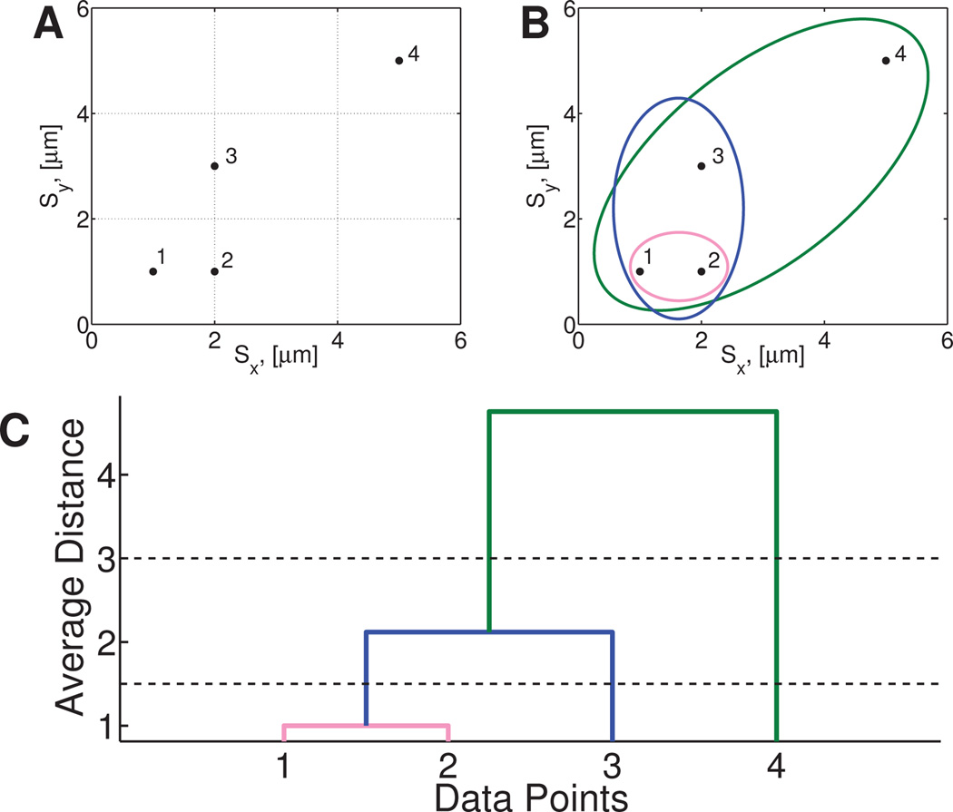
The pairwise distances between all scalar pairs $(s_x^j(\tau ),s_y^j(\tau ))$ is calculated using the Euclidean distance metric and the distance between clusters is determined by computing the average distance between all points in both clusters, a metric known as the average linkage function. In agglomerative hierarchical clustering, each data point is initially its own cluster. The two closest clusters based on the Euclidean distance in $(s_x^j(\tau ),s_y^j(\tau ))$ space (points 1 and 2 in Figure 1B) are then merged to form a new cluster (pink cluster). This process is repeated (blue cluster containing points 1, 2 and 3, Figure 1B) until all of the data points have been merged into a single cluster (green cluster containing all points, Figure 1B). Recording the order in which clusters are merged allows one to construct a dendrographic representation of the data (Figure 1C), showing the hierarchical similarity between clusters.³⁵ The height of each connection in the dendrogram is equal to the average distance between the connected clusters, encoding a hierarchical metric of cluster similarity based on their van Hove correlation functions.

Fig. 1. Example of hierarchical clustering.

A) The distribution of data points to be clustered. Each data point is assigned to a cluster containing only itself. The pairwise distances between all clusters are calculated and the closest two clusters are merged to form a new cluster. B) This process is repeated until all data points are in a single cluster. C) A dendrogram shows the distances between each cluster and the order in which they were merged. The solid lines at 3 and 1.5 show cutoff values that produce two and three clusters, respectively.

After all the distances are calculated (Figure 1C), the number of clusters, K_τ, is determined by a cutoff value ζ that partitions the dendrogram at resolution ζ. For instance, if we choose any ζ < 1 in Figure 1, all particles remain in their own cluster, and there are 4 clusters at this resolution. For any 1 < ζ < 2.12, say ζ = 1.5 as in Figure 1C, the two points making up the pink cluster are now indistinguishable. Thus we declare 3 clusters for this range of ζ. Next, for 2.12 < ζ < 4.75, there are only 2 clusters, the blue cluster and point 4, as shown in the figure for ζ = 3. Finally, for ζ > 4.75, there is one cluster with that chosen degree of resolution, the green cluster containing all points. In this way, the parameter ζ solely determines the partitioning of the data, and as ζ varies from the smallest to largest values, the number of clusters K_τ spans 1 to N, where N is the number of observed particles. The next critical step is to select the degree of resolution, i.e. the value of ζ, and thus to determine the number of clusters K_τ that best delineates the ensemble of paths at lag time τ.

4.2.2 Optimal number of clusters and the gap statistic

To find the optimal number of clusters, $K_{\tau }^{*}$, we use a gap statistic.²⁰ We start by defining the parameter W_K as²³

$$W_K(K_{\tau })=\mathrm{\sum }_{c=1}^{K_{\tau }}\frac{1}{2n_c}{D}_c,$$ (9)

where n_c is the number of elements in cluster c and D_c is the sum of the pairwise squared distances between all the elements of cluster c. As ζ decreases, the number of clusters, K_τ, increases, which in turn results in a decrease of W_K due to the increasing mean intra-cluster density.

Next, we use these values of W_K to compare the distribution of standard deviations of the van Hove functions, which may or may not contain statistically distinct clusters, to a null reference data set containing only one cluster and with uniform density. In order to ensure that the null reference data set only contains a single cluster with uniform density, this data is generated from a uni-modal uniform distribution. To match the input data as closely as possible (apart from the number of clusters present), the reference data set is created such that its cardinality and domain are the same as the input data, i.e. the distribution of $(s_x^j(\tau ),s_y^j(\tau ))$. To remove the variability and arbitrariness associated with the comparison of the input data to a single reference data set, it is common practice to compare the input data to multiple reference data sets. We have determined that 100 reference data sets suffices to consistently partition the data.

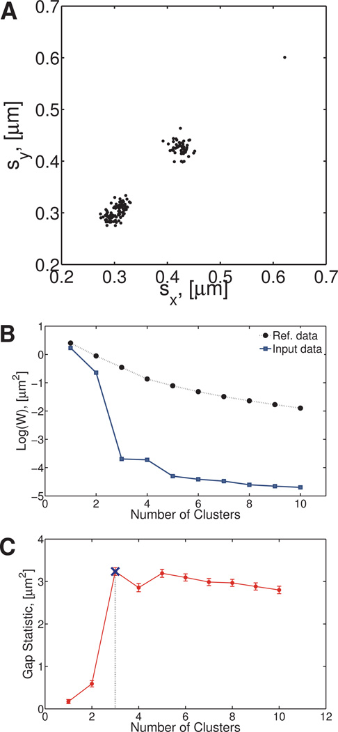
To illustrate this procedure, we numerically generate paths of 150 1-µm diameter spherical particles diffusing via Brownian motion in a heterogeneous medium with diffusion coefficients: 1.28 (50 paths), 1.49 (50 paths), 2.72 (49 paths), and 3.10µm²/s (1 path). This data set will be referred to as the “Numerically Generated Heterogeneous Newtonian” (NGHN) data set. First we fit the van Hove correlation function of each particle path to a Gaussian, doing so separately for each coordinate, and thereby recording standard deviation of each particle’s x and y step size distributions. For particle diffusion in a viscous fluid, the van Hove correlation function in any direction has mean 0 and variance s(τ) where $s(\tau )=\sqrt{2D\tau }$, and the diffusion coefficient is given by the Stokes-Einstein relation,

$$D=\frac{k_{B}T}{6\pi \eta a},$$ (10)

where a is the particle radius and η is the fluid viscosity. In our example, the resulting distribution of standard deviations, $(s_x^j(\tau ),s_y^j(\tau ))$, is shown in Figure 2A. We next calculate W_K for the path data and W_ref, which is the mean of the W_K‘s calculated using Eqn. (9) in each of the 100 reference data sets described previously. These results are plotted in Figure 2B as a function of the number of clusters, K_τ. A measure of the variability introduced by the use of a finite number of reference data sets has the form $s_K=\mathit{\text{sd}}(K)\sqrt{1+1/B}$, where sd is the standard deviation of the reference data set and B the number of sets.²⁰

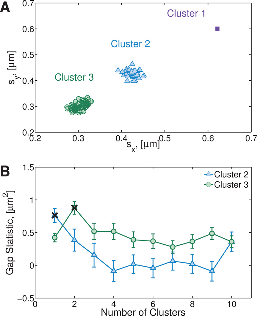
Fig. 2. First clustering step on the Numerically Generated Heterogeneous Newtonian (NGHN) data set.

A) Standard deviations of van Hove functions for particles moving in a Newtonian, heterogeneous fluid. The heterogeneity of the fluid is characterized by four different diffusion coefficients. B) Value of W is given by Eqn. (9), the gap statistic is calculated based on the differences between the reference and input data. C) Gap statistic calculated as described in Section 4.2.2. This statistic indicates that initially there are three clusters in the sample.

We are interested in the change in log(W_K) relative to log(W_ref) for increasing K_τ. The difference between these data sets, known as the gap statistic, was proposed by Tibshirani et al,²⁰ to formalize the observation that the point at which the rate of change of log(W_K) significantly increases is an indicator of the “true” number of clusters in the data. We acknowledge the alternative form of the gap statistic comparing W_K and W_ref without the logarithm, but have opted not to use it because of the documented decrease in performance when analyzing overlapping clusters.²³

The optimal number of clusters in the distribution of standard deviations of van Hove functions, for a given lag time, is estimated as

$$K_{\tau }^{*}=\underset{K_{\tau }}{\text{argmin}}\{K_{\tau }|G(K_{\tau })\ge G(K_{\tau }+1)-s_{K_{\tau }+1}\},$$ (11)

where argmin returns the value of the input argument that minimizes the input function. This equation chooses $K_{\tau }^{*}$ to be the smallest number of clusters such that the value of the gap statistic at K_τ clusters is greater than or equal to the lower bound of the gap statistic when K_τ + 1 clusters are present. In our example, at this stage of the algorithm, three clusters are identified $K_{\tau }^{*}=3$ as shown in Figure 2C.

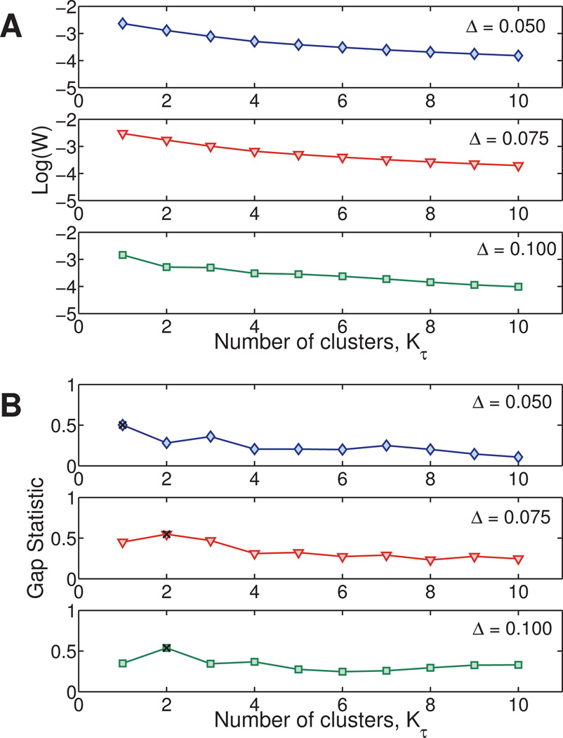
It is clear from these results that at this stage the algorithm fails to distinguish between the two clusters that are closest together. A question arises as to what is the minimal ‘separation’ in variances of the step size distribution between two clusters so that they appear as distinct in this step. Recall that in our example, this is the same as asking what minimum difference in diffusivities is distinguishable by these metrics. To investigate this, we generated three heterogeneous Newtonian data sets of size N = 200. Each data set contains two clusters: particles belonging to the first cluster have diffusivity D₁ = 1.61 × 10⁻²µm²/s, while particles in the second cluster have diffusivity D₂ = D₁ (1 + Δ). The value D₁ is the diffusion coefficient of a one-micron particle diffusing in a medium with viscosity 27 mPa s. We choose three values of Δ: 0.05, 0.075, 0.10. Our algorithm correctly identifies the two clusters when Δ ≥ 7.5%. We note that the NG_τ (Eqn. 2) metric, the heterogeneity ratio (Eqn. 4) and the percent contribution of the bin partitions described by Tseng et al.⁴⁵ steadily increase as Δ increases, as expected for increasing heterogeneity. The Stage 2 metric of Valentine et al.²⁴ identifies two to three clusters in each data set. These results are given in Table S1 of the Supplemental Material.

Given these results from other methods in the literature, we now apply our method. Figure 3A shows values of log(W_K) vs K_τ for each of the four data sets. As Δ increases, the ‘bend’ in the plot at K_τ = 2 becomes more pronounced. Figure 3B shows the gap statistic as a function of K_τ. The optimal number of clusters $K_{\tau }^{*}$ is indicated by a black X. We see that for a Newtonian fluid in this range of diffusivities, the distribution of the standard deviations of the van Hove correlation functions of two data sets with diffusivities that vary by only 5% are indistinguishable. However as the difference in the diffusivities increases to 7.5% and beyond, the distributions become distinguishable by our metrics and the correct number of clusters is successfully recovered. It is important to point out that this 7.5% threshold may not hold for different data sets and its value depends on, among other variables, the total number of clusters, presence of outliers, distribution of points within each cluster, and experimental error.

Fig. 3. Test of the gap statistic test: numerical data with controlled degrees of heterogeneity in the diffusion coefficients.

Four heterogeneous Newtonian data sets are generated, where each data set consists of 200 paths of particles of diameter 1 µm. For each data set, the first 100 paths have diffusion coefficient D₁ = 1.61 × 10⁻²µm²/s while the next 50 paths have diffusion coefficient D_Δ = D₁ (1 + Δ) for Δ = 5%,7.5%, and 10%. A) As Δ increases, the ‘bend’ in the log(W) vs. K_τ plot at K_τ = 2 becomes more pronounced. B) The gap statistic correctly indicates two clusters for Δ ≥ 0.075. The number of clusters selected by the gap statistic is indicated by a black ×.

4.2.3 Optimization of initial clustering based on different lag times

In Section 4.2.2 we showed how to select the optimal number of clusters for a given lag time, τ. In this section, we address the fact that the optimal number of clusters might change as the lag time is varied. For this, the clustering process introduced in Section 4.2.2 is applied to each distribution of standard deviations, $(s_x^j(\tau ),s_y^j(\tau ))$, for a selected number of lag times. Each set of lag times is obtained as a linear distribution from τ₁ to τ₁₀ = 100/δ s, in increments of 10/δ s. Here, τ₁ is the smallest lag time on a given data set and δ the frame rate (fps).

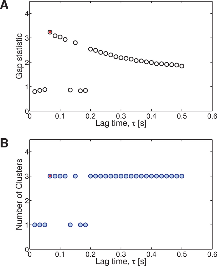
As τ changes, the optimal number $K_{\tau }^{*}$ of clusters at a particular lag time varies, and the cluster assignment of each particle may therefore change as well. To choose among these partitions of the data, we select the clustering with the smallest value of τ that maximizes $K_{\tau }^{*}$. This value will be referred to as K^†. Recall that as τ increases, the number of data points used in the van Hove correlation decreases. By selecting the smallest value of τ that maximizes the heterogeneity, we are maximizing our confidence in each data point $(s_x^j(\tau ),s_y^j(\tau ))$ and therefore our confidence in the accuracy of the clustering. Figure 4A shows the value of the gap statistic at $K_{\tau }^{*}$ for each lag time τ, while Figure 4B shows the number of clusters $K_{\tau }^{*}$ found at each lag time. In these figures, K^† is indicated by a red circle and corresponds to a lag time of 0.067 s. From this point forward, any further division of the data will be performed using the van Hove correlation function corresponding to τ^† = 0.067 s.

Fig. 4. Optimization of initial clustering based on different lag times for the Numerically Generated Heterogeneous Newtonian data set.

(Section 4.2.3) A) The value of the gap statistic at $K_{\tau }^{*}$ is shown for each lag time. B) The optimal number of clusters is determined from the smallest lag time that gives the largest number of clusters (red dot).

4.2.4 Cluster refining

After the main clusters are identified, we repeat the hierarchical clustering and gap statistic steps for each cluster c = 1,..,K^†. The first clustering steps (Sections 4.2.1–4.2.3) serve to identify well-separated clusters while the second round of clustering, introduced here, inspects each previously identified cluster for the presence of sub-clusters. The final number of clusters K^final is the total number of clusters found after applying the clustering algorithm to each of the previously identified K^† clusters. This two-pass clustering is robust to outliers that normally causes single-pass clustering to fail. Figure 5A shows the three clusters previously identified (K^† = 3). The clustering steps described in Sections 4.2.1–4.2.3 are repeated for each individual cluster with size n_c > 3 and the resulting gap statistics are shown in Figure 5B.

Fig. 5. Cluster refining on the Numerically Generated Heterogeneous Newtonian data set.

(Section 4.2.4) A) Resulting clusters from initial clustering step. B) The clustering algorithm is applied to each individual cluster to identify any sub clusters. In this example, Cluster 3 is subdivided into two groups, while Cluster 2 remains a single group. Cluster 1 contained a single point, therefore no further analysis is needed.

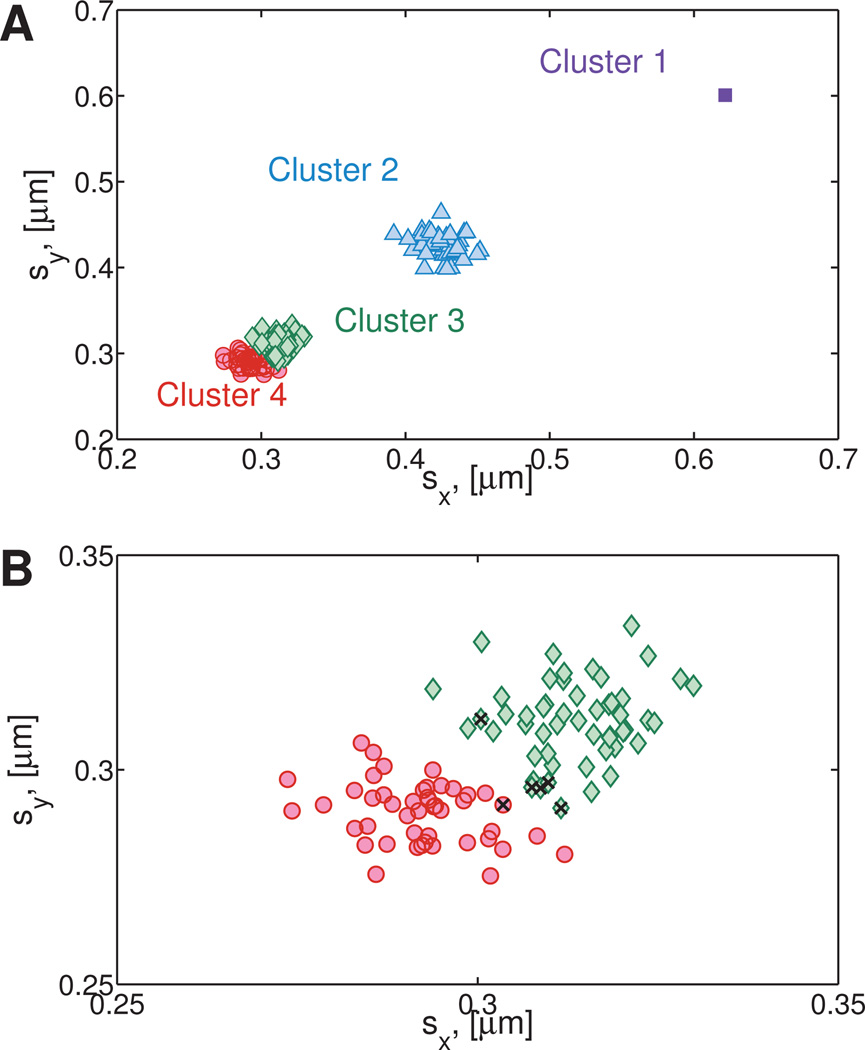
From Figure 5B it is clear that Cluster 3 is composed of two sub-clusters giving a total of four clusters (K^final = 4), shown in Figure 6A. Figure 6B shows the resulting division of cluster 3 into two sub-clusters.

Fig. 6. Final number of clusters for the Numerically Generated Heterogeneous Newtonian data set.

A) Total number of clusters identified by the algorithm described in Section 4.2. Note that Cluster 1 is identified as an outlier, since it contains less than 3 points. B) Detailed view of Cluster 3 and 4. Since the data is simulated, it is easy to check whether points are placed in the wrong cluster. These points are indicated in the figure by a black ×. Six points out of 150 were misclassified.

4.3 Cluster distribution fitting

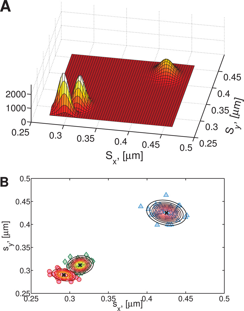
Once the data has been fully partitioned, i.e., we have K^final, we assume that the distribution of standard deviations of the van Hove correlation functions, $(s_x^j({\tau }^{\mathrm{†}}),s_y^j({\tau }^{\mathrm{†}}))$ can be described by a Gaussian mixture model²¹ where the data points within each cluster are normally distributed. To ascertain the statistical significance of each cluster, i.e., the probability that each point is a member of a given cluster and the parameters that describe the Gaussian mixture model, we employ an iterative machine learning algorithm known as an Expectation-Maximization (EM) algorithm.³⁴ The EM algorithm is chosen because it is numerically stable and the computation time per iteration is relatively small. We initialize the EM algorithm by calculating a vector of means µ and a covariance matrix Γ for each cluster. Each component of the Gaussian mixture is of the form,

$$f(s|\mu ,\mathrm{\Gamma })\mathrm{\propto }\text{exp}[-\frac{1}{2}(s-\mu )\prime {\mathrm{\Gamma }}^{-1}(s-\mu )],$$ (12)

where s is shorthand for the N × 2 vector of standard deviations of the van Hove distribution $[s_x^j({\tau }^{\mathrm{†}}),s_y^j({\tau }^{\mathrm{†}})]$. The EM algorithm determines the parameters of the Gaussian mixture that best fits the data by maximizing the log likelihood of generating the data given a set of parameters. For further description of the EM algorithm the reader is referred to the works of Hastie et al.²² and Bishop.²¹ In addition, any cluster with fewer than three points is not considered during the EM phase. In our extended example on the NGHN data, this means we only apply the EM algorithm to the ensemble of clusters 2, 3 and 4, omitting the single point which forms Cluster 1. Figure 7A shows the three-component 2D probability distribution resulting from the EM algorithm. Given the location of the center of each cluster, the Gaussian parameters for each component can be used to measure the relative strength of each particle’s cluster assignment, i.e., the probability that any given point is a member of each cluster.

Fig. 7. Gaussian mixture fitting on the Numerically Generated Heterogeneous Newtonian data set.

A) 2-D probability distribution of the center of each cluster. B) Isoclines of each Gaussian component and cluster centers (black ×) overlaid on 2D distribution of standard deviations of individual van Hove functions.

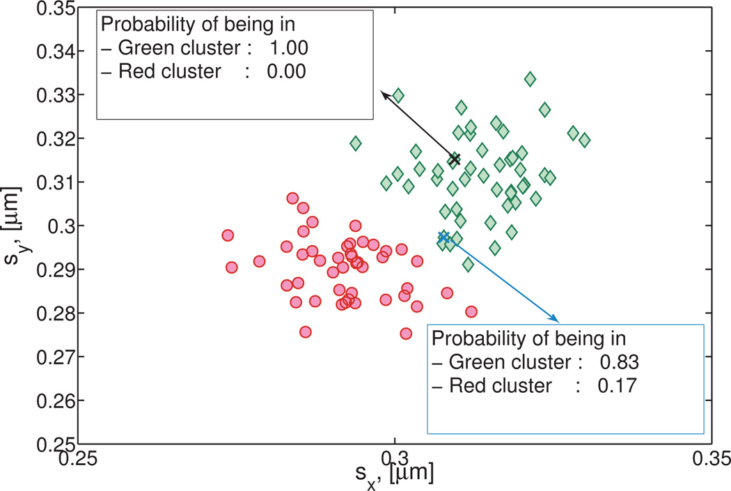
While two points may be assigned to the same cluster, the probability that such an assignment is correct depends on the location of that point relative to the cluster center. This is illustrated in Figure 8 for two points. Given the stochastic nature of particle diffusion, it is possible to erroneously assign particles to a cluster (see for example Figure 6B). Therefore, determining these probabilities is an important step to evaluate the use of a given particle path in the analysis of a specific cluster’s properties. Certainly, the level of refinement required depends on the particulars of the application.

Fig. 8. Detail of Cluster 3 and Cluster 4 from Figure 7 and the Numerically Generated Heterogeneous Newtonian data set.

With the EM algorithm explained in Section 4.3, the probability that each point is a member of each cluster is calculated by evaluating all Gaussian components of the Gaussian mixture model at each point, $(s_x^j({\tau }^{\mathrm{†}}),s_y^j({\tau }^{\mathrm{†}}))$.

4.4 Algorithm to simulate numerical data

For the purpose of validating the protocol described in Sections 4.1–4.3, we perform simulations of particles moving both by regular Brownian motion and by fractional Brownian motion (fBm). fBm^57,58 is a self-similar Gaussian process with stationary increments and mean squared displacement given by,

$$\langle \mathrm{\Delta }{r}^2(\tau )\rangle =2d{D}_{\text{fBm}}{\tau }^{\alpha },$$ (13)

where α is the power law exponent 0 ≤ α ≤ 2, D_fBm is the generalized diffusion coefficient with dimensions L^2/tα and d is the dimensionality of the data. In the probability literature, the exponent α is replaced by H = 2α and called the Hurst parameter. The autocorrelation function for fBm has long-range correlations,

$$\langle {\xi }_{\alpha }(0){\xi }_{\alpha }(t)\rangle \approx \alpha (\alpha -1)t^{\alpha -2},$$ (14)

where ξ_α is the fractional Brownian noise. This class of processes generalizes regular Brownian motion, which corresponds to α = 1, the only value for which the motion is uncorrelated. For 0 < α < 1 the pre-factor in Eqn. (14) is negative so that the increments are negatively correlated, rendering the associated process sub-diffusive. Conversely, when α > 1 the motion is persistent (positively correlated), resulting in superdiffusion in which successive steps are biased toward follow in the same direction. Subdiffusive fBm has been used to model a variety of processes including diffusion of 1-micron diameter particles in HBE mucus,⁶ diffusion of biopolymers inside cells,³⁶ monomer diffusion in a polymer chain,⁵⁹ bacteria chromosomal loci,³⁷ polymer translocation,⁶⁰ and diffusion in crowded fluids.⁶¹ We have selected fBm as a model based on its ability to describe the autocovariance observed in the displacements of particles undergoing passive thermal diffusion in a wide range of both simple and complex fluids (See for example supplemental Figure 1).

4.4.1 Generating particle paths

Given the covariance matrix

$${\mathrm{\Lambda }}_{i,j}=\frac{1}{2}(t_i^{\alpha }+t_j^{\alpha }-{|t_i-t_j|}^{\alpha }),$$

for i,j = 1, …,M, define R² = Λ. A particle path is generated as $\mathbf{X}=\sqrt{2D_{\text{fBm}}}(\mathbf{\text{uR}})$, where u is a 1 × M vector of normally distributed random numbers with zero mean and unit variance. ^62–63 The distribution of step sizes dx_i = x(1 + iτ) –x(1 + (i − 1)τ) has standard deviation, σ_τ, explicitly given by

$${\mathrm{\sigma }}_{\tau }=\sqrt{2D_{\text{fBM}}{\tau }^{\alpha }}.$$ (15)

Note that in simulations for regular Brownian motion, we only need to calculate the vector u, since Λ becomes the identity matrix.

The mean fBm parameters, D_fBm and α, are calculated on a per-cluster basis for each of the K^final clusters. A builtin MATLAB solver for constrained nonlinear optimization is used to estimate D_fBm and α using Eqn. (15). It is important to emphasize that while K^final is determined at a particular value of τ, the fitting procedure must be carried out over multiple values of τ. This is due to the fact that for a given τ and σ_τ, there is a one-dimensional curve of (D_fBm,α) pairs which satisfies Eqn. (15).

4.5 Metric Comparison

When our algorithm is applied to the numerically generated heterogeneous Newtonian (NGHN) data set (Figures 2–8), we find three main clusters corresponding to the three clusters generated with mean diffusivities 1.28, 1.49, and 2.72 µm²/s. The outlying point, generated with D = 3.10µm²/s, was also correctly identified. Following Section 4.4 we assume fBm as the underlying process, and fit D_fBm and α for the three main clusters. The mean error in the predicted value of D_fBm across all clusters is 2.8%. The mean error in the predicted value of α across all clusters is 0.96%. To compare the performance of our algorithm with the metrics described in Section 2, we applied those metrics to this same set of data.

All Stage 1 metrics presented in Section 2.1 correctly indicated that the simulated data set was heterogeneous. The non-Gaussianity parameter (Eqn. 2), excess kurtosis (Eqn. 3), and heterogeneity ratio (Eqn. 4), are 0.19, 0.58 and 13.0, respectively. The relative contributions of the 10%, 25% and 50% highest values of the individual compliance to the ensemble mean compliance were 17%, 38% and 64%, respectively. Finally, the mean spatial relative standard deviation in the iMSD amplitudes was 1.02.

The Stage 2 metric of Valentine et al.²⁴ described in Section 2.2 was applied to the simulated data set multiple times. Clusters were formed by randomly selecting “representative” particle paths of the particles not yet clustered and assigning all particle paths to a cluster based on the results of an F-test. In each instance, the data was correctly determined to be heterogeneous while the number of statistically distinct clusters within the data predicted by the algorithm varied between 6 and 7. However, particle assignments to these clusters varied (Figure 9), demonstrating sensitivity to the choice of the representative particle path. We note that this is one of the main advantages of our algorithm, in our case particles are uniquely assigned to a cluster.

Fig. 9. Sample results of the metric proposed by Valentine et al²⁴ for the Numerically Generated Heterogeneous Newtonian dataset.

The choice of order in which the particles are compared results in different numbers of clusters and cluster distributions. For example, six clusters were found in A, while in B seven clusters were identified.

5 Results and Discussion

We set out to test our methods on a variety of simulated and experimental data sets exhibiting various degrees of heterogeneity. In each instance, the simulated data was generated with parameter values comparable to the measured values for the corresponding experimental data set. This provides a way to distinguish the error inherent in our algorithm from experimental error.⁶⁴

5.1 Homogeneous data: Numerical and Experimental

5.1.1 Newtonian Paths and Data Analysis

(a) Numerical

100 particle paths were generated with α = 1 and D_fBm = 1.61 × 10⁻²µm²/s. These values of D_fBm and α were chosen to match the expected values for the experimental homogeneous sucrose data. See Table S2 for the resulting best fit values of α and D_fBm and their corresponding 95% confidence intervals.

(b) Experimental

Position time series were collected for 100 1-µm diameter particles undergoing passive thermal diffusion in a 2 molar sucrose solution. The viscosity of the 2 molar sucrose solution was calculated to be 0.027 Pa s based on the MSD of embedded tracer particles. See Table S3 for the resulting best fit values of α and D_fBm and their corresponding 95% confidence intervals.

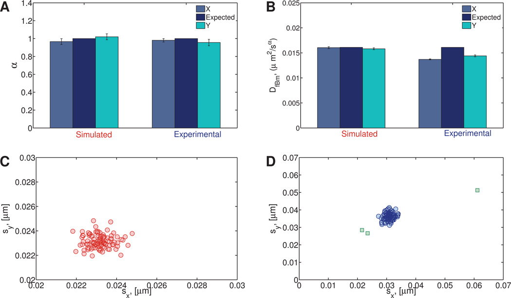
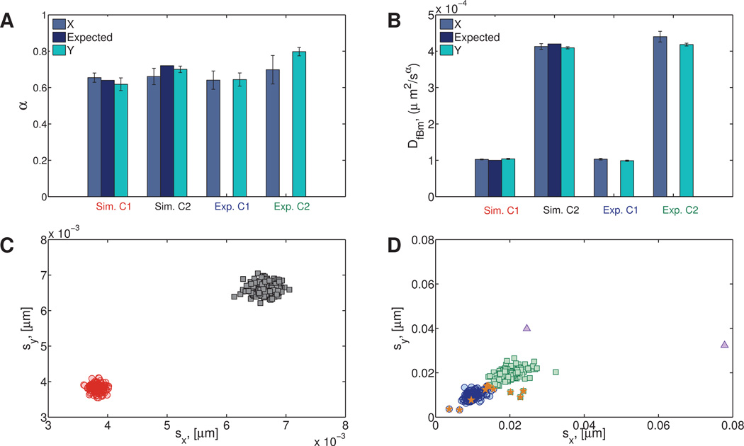
The results from our clustering algorithm and subsequent fitting to Eqn. (15) for the homogeneous numerical and experimental Newtonian data sets are shown in Figure 10A and B for α and D_fBm, respectively.

Fig. 10. Simulated and experimental (sucrose) homogeneous Newtonian data.

Panels A and B show the expected and inferred fBm parameters, α and D_fBm. The distribution of standard deviations of the van Hove correlation functions for the simulated and experimental data are shown in panels C and D, respectively. The squares in panel D indicate points that have been classified as outliers.

The 95% confidence intervals (CI₉₅) for α in the x direction was (0.933,0.998) for the simulated data compared to (0.961,1.00) for the experimental data. Similarly, the CI₉₅ for the x component of D_fBm is (1.59 × 10⁻²,1.62 × 10⁻²), while the experimental CI₉₅ is (1.36 × 10⁻²,1.38 × 10⁻²). Confidence intervals for all other data sets can be found in the supplemental materials.

For the data presented here, as well as in Section 5.2.1, a modified fitting procedure for D_fBm was implemented. Once α was determined to be sufficiently close to 1, that is the process is indistinguishable from simple Brownian motion, D_fBm was calculated with α fixed at exactly 1. The resulting diffusion coefficients yield the viscosity of the fluid through the Stokes-Einstein relation, Eqn. (10). For the homogeneous data, the expected values of D_fBm were comparable, D_fBm,x = 1.37 × 10⁻²µm²/s^α and D_fBm,x = 1.36 × 10⁻²µm²/s for non-fixed and fixed α cases, respectively. However, because of the decrease in the degrees of freedom in the fitting process that occurs when α is fixed, the 95% confidence interval is larger when α is fixed (Table S4).

5.1.2 Viscoelastic Paths and Data Analysis

(a) Numerical

175 particle paths were generated with α = 0.576 and D_fBm = 9.30 × 10⁻⁵ µm²/s^α. These values of D_fBm and α were chosen to match the inferred experimental values of D_fBm and α for homogeneous HA path data. See Table S5 for the resulting best fit values of α and D_fBm and their corresponding 95% confidence intervals.

(b) Experimental

Position time series were collected for 175 1-µm particles undergoing passive thermal diffusion in a 10mg/ml HA solution. See Table S6 for the resulting best fit values of α and D_fBm and their corresponding 95% confidence intervals.

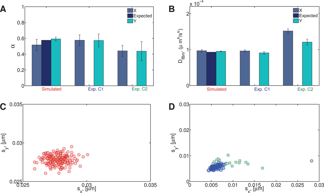
The results for the experimental viscoelastic data (Figures 11A–B) indicate the presence of two clusters, even though only one cluster was expected. Further inspection shows that the second cluster in the experimental data (Exp. C2) contains 14 data points representing 18% of the particles. Figure 11D shows the standard deviations s_x, s_y of the x and y components of these paths. Whereas the protocol for preparation of the HA solution is expected to yield a homogeneous mixture, the data analysis reveals a likelihood of imperfect mixing and therefore a mildly heterogeneous fluid.

Fig. 11. Simulated and experimental (hyaluronic acid) homogeneous viscoelastic data.

A) Power law exponent and B) fractional diffusion coefficient distributions. C) Standard deviations of simulated data. D) Standard deviations of experimental data. For the experimental hyaluronic acid data, the main cluster (denoted Exp. C1) contains 161 data points and is shown in blue (open circles). The second cluster (Exp. C2) contains 14 data points and is shown in green (open squares). One statistically distinct outlier was also found (gray circle).

5.2 Heterogeneous data: Numerical and Experimental

5.2.1 Newtonian Paths and Data Analysis

(a) Numerical

90 particle paths were generated with α = 1 and D_fBm = 8.05 × 10⁻³µm²/s and combined with 100 particles generated with α = 1 and D_fBm = 1.61 × 10⁻²µm²/s. These values of D_fBm and α were chosen to match the expected values for the heterogeneous experimental sucrose data containing 1-µm and 2-µm diameter beads. See Table S7 for the resulting best fit values of α and D_fBm and their corresponding 95% confidence intervals.

(b) Experimental

Position time series were collected for 90 2-µm diameter particles in 2 molar sucrose solution and combined with the 1-µm experimental data presented in Section 5.1.1. See Table S8 for the resulting best fit values of α and D_fBm and their corresponding 95% confidence intervals.

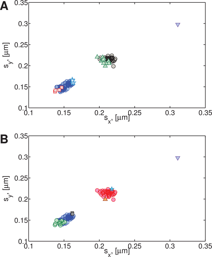
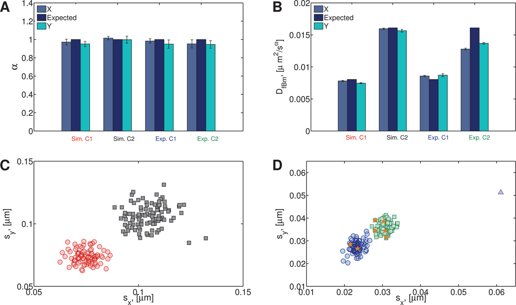
For both the simulated and experimental Newtonian data, the correct number of clusters (2) was found. After the experimental data were processed, by cross referencing the cluster assignments with the file that the data came from, we were able to determine that 7 out of the 190 data points (Figure 12D) were assigned to the wrong cluster.

Fig. 12. Simulated (Sim.) and experimental (sucrose) (Exp.) heterogeneous Newtonian data arising in both datasets from bi-disperse particle diameters of 1 and 2 microns as a proxy for bi-disperse fluid viscosities.

A) Distributions of power law exponent and B) fractional diffusion coefficient. C) Standard deviations for the simulated data. D) Standard deviations for the experimental data. The data points that have been assigned to the wrong cluster are indicated with an orange star. One statistically distinct outlier was also found (triangle).

5.2.2 Viscoelastic Paths and Data Analysis

(a) Numerical

180 particle paths were generated with α = 0.64 and D_fBm = 100 × 10⁻⁴µm²/s^α and combined with 180 particle paths generated with α = 0.72 and D_fBm = 4.20 × 10⁻⁴×µm²/s^α. These values of D_fBm and α represent the best-fit values for the two experimental data sets on HA just below, taken from Table S11. Table S10 provides the resulting best fit values of α and D_fBm after clustering for these numerically generated paths, and their corresponding 95% confidence intervals.

(b1) Experimental (HA solutions)

The 175 1-µm diameter particles in 10mg/ml HA solution presented in Section 5.1.2 were combined with data for 188 1-µm particles undergoing passive thermal diffusion in a 8mg/ml HA solution. Table S11 provides the resulting best fit values of α and D_fBm after clustering these experimental paths, and their corresponding 95% confidence intervals.

The algorithm correctly resolved the number of clusters in each data set. All paths were correctly classified in the simulated data while 11 out of 363 experimental paths were misclassified, including two outlier paths, Figure 13D. Comparison of the best-fit fBm parameters in this experimental-numerical exercise with hyaluronic acid solutions reveals the uncertainty associated with experimental noise or outliers, and with choosing an ad hoc model to fit to the data.

Fig. 13. Simulated and experimental (hyaluronic acid) heterogeneous viscoelastic data, where heterogeneity is controlled by use of identical 1 micron particles in two different concentrations, 8 and 10 mg/ml, hyaluronic acid.

A) Power law exponent and B) fractional diffusion coefficient distributions. C) Standard deviations of simulated data. D) Standard deviations of experimental data. The data points that have been assigned to the wrong cluster are indicated with an orange star. Two statistically distinct outliers were found (triangles).

We now apply our clustering algorithm to path data from two putatively heterogeneous complex fluids with unknown heterogeneity. To our knowledge, there is no guidance in the literature for a quantitative heterogeneous characterization of agarose solutions or HBE cell culture mucus.

(b2) Experimental (0.2% w/w agarose)

Position time series were collected for 38 1-µm particles undergoing passive thermal diffusion in a 0.2% agarose solution. See Table S12 for the resulting best fit values of α and D_fBm and their corresponding 95% confidence intervals.

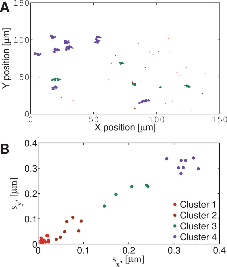
The results from a 0.2% w/w agarose solution are shown in Figure 14. It is clear from Figure 14A that the ensemble of particles exhibit a range of diffusive behavior, from relatively mobile to nearly immobile. These disparities in diffusive behavior are resolved with our clustering methods into four distinct clusters, Figure 14B. The path data for each cluster is then fit to fractional Brownian motion, with the results shown in Table S12 in Supplemental Material. The highest percentage of paths belong to cluster one (18 paths) while clusters two, three, and four have 7, 5, and 8 paths, respectively. We note that cluster 4 has α ≈ 1 which indicates those beads are moving in a Newtonian environment, and D_fBm ≈ 0.1µm²/s indicates that this environment has an effective viscosity of 4.4 mPa s. Clusters 1–3 reflect sub-diffusion with α < 1; in particular, cluster 1 has an fBm exponent α = 0.1 indicating that these beads are effectively immobilized.

Fig. 14. Experimental Agarose data: position time series in physical space and results of cluster analysis.

1 µm diameter beads diffusing in 0.2% w/w agarose. A) Particle paths in two space dimensions of the microscope focal plane, with color coding inserted after cluster analysis. B) Results from the clustering algorithm, revealing four clusters. Cluster assignments are then carried back to the physical locations in the focal plane in Figure 14A

(b3) Experimental (2.0% w/w HBE cell culture mucus)

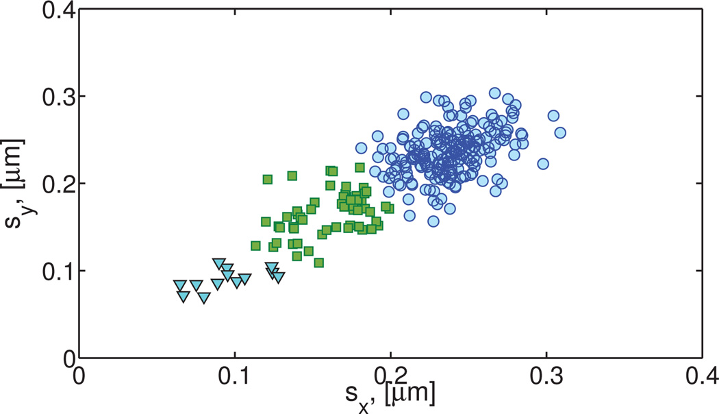
Position time series were collected for 282 0.5-µm particles undergoing passive thermal diffusion in a 2.0% HBE mucus. See Table S13 for the resulting best fit values of a and D_fBm and their corresponding 95% confidence intervals. The resulting clusters are shown in Figure 15.

Fig. 15. Clustering of experimental HBE mucus data.

0.5 µm diameter beads diffusing in 2% w/w HBE mucus.

The protocol reveals three clusters. The resulting power law exponents and pre-factors are given in Table S13 of the Supplemental Material. These results reveal that all probes exhibit sub-diffusive motion with the majority of beads (215 in cluster 3) having α ≈ 0.6 and D_fBm ≈ 2.4 × 10⁻⁴µm²/s^0.6. Clusters 2–3 have, respectively, 13 and 59 paths each.

6 Conclusions

A protocol for analysis of path data from passive particle tracking microrheology, is presented that yields a quantitative characterization of diffusive heterogeneity in complex fluids. This protocol is based on methods adapted from the statistics and machine learning literature. The first goal is to design an algorithm to quantify the observed heterogeneity based on the primitive path data, without reliance on a presumed model of the underlying stochastic process, beyond the minimal assumption that the increments of single paths are stationary and Gaussian. The second goal is to have a technique that yields unique, reproducible clustering of the given ensemble of paths. Similar to other approaches discussed in Section 2, our algorithm is applied to the position time series of passive particles in simple or complex fluids. Specifically, we partition the paths into clusters whose step-size distributions are statistically distinct, which may arise either due to differences in particle characteristics or complex fluid characteristics, or both. Using the standard deviation of the van Hove correlation function as our metric of interest and two-pass hierarchical clustering with the gap statistic to partition the data, our algorithm yields a robust and consistent method for the detection and quantification of heterogeneity in complex fluids. The method to this point is weakly parametric, only relying on the assumption that each path is stationary and the increments are Gaussian. After the clustering step is complete, our protocol fits the parameters of a proposed model on a per-cluster basis, which we have illustrated for simple Brownian motion and fractional Brownian motion, on both numerical and experimental data.

To benchmark our algorithm, we created data sets containing known, discrete levels of heterogeneity. We analyzed experimental data with “artificial” heterogeneity using two methods. For analysis of heterogeneity in Newtonian fluids, we embedded particles of two different diameters in a homogeneous solution (Section 5.2.1). For analysis of heterogeneity in viscoelastic fluids, identical particles were embedded in two hyaluronic acid solutions of different concentrations and then the path data was combined into one dataset (Section 5.2.2). For Newtonian fluids, doubling particle diameter is a proxy for doubling viscosity, or equivalently halving the diffusion coefficient. In addition to controlling the degree of heterogeneity in the paths, combining dissimilar data sets provides us with a way to test the accuracy of our particle-cluster assignments. Finally, we applied our protocol to monodisperse particles in two putative heterogeneous complex fluids, an agarose gel and mucus derived from human bronchial epithelial cell cultures. The data analysis reveals that both fluids are heterogeneous, and indicates a quantitative variability in sub-diffusive behavior that would have strong implications for passage times through mucus barriers.

The accuracy of our method, the small necessary volume of fluid, and the short collection times required to quantify the heterogeneous composition of viscous and viscoelastic samples, combine to make our methods promising for a wide range of applications in PPTM.

References

- 1.Wirtz D. Annu Rev Biophys. 2009;38:301–326. doi: 10.1146/annurev.biophys.050708.133724. [DOI] [PubMed] [Google Scholar]
- 2.Lai SK, Wang Y-Y, Wirtz D, Hanes J. Adv Drug Delivery Rev. 2009;61:86–100. doi: 10.1016/j.addr.2008.09.012. [DOI] [PMC free article] [PubMed] [Google Scholar]
- 3.Matsui H, Verghese MW, Kesimer M, Schwab UE, Randell SH, Sheehan JK, Grubb BR, Boucher RC. J Immunol. 2005;175:1090–1099. doi: 10.4049/jimmunol.175.2.1090. [DOI] [PubMed] [Google Scholar]
- 4.Matsui H, Wagner VE, Hill DB, Schwab UE, Rogers TD, Button B, Taylor RM, Superfine R, Rubinstein M, Iglewski BH, et al. Proc Natl Acad Sci USA. 2006;103:18131–18136. doi: 10.1073/pnas.0606428103. [DOI] [PMC free article] [PubMed] [Google Scholar]
- 5.Kesimer M, Ehre C, Burns KA, Davis CW, Sheehan JK, Pickles RJ. Mucosal Immunol. 2012;6:379–392. doi: 10.1038/mi.2012.81. [DOI] [PMC free article] [PubMed] [Google Scholar]
- 6.Hill DB, Vasquez PA, Mellnik J, McKinley S, Vose A, Mu F, Henderson AG, Donaldson SH, Alexis NE, Boucher R, Forest MG. PLoS ONE. 2014;9:e97980. doi: 10.1371/journal.pone.0087681. [DOI] [PMC free article] [PubMed] [Google Scholar]
- 7.Waigh TA. Rep Prog Phys. 2005;68:685–742. [Google Scholar]
- 8.Cicuta P, Donald AM. Soft Matter. 2007;3:1449–1455. doi: 10.1039/b706004c. [DOI] [PubMed] [Google Scholar]
- 9.Squires TM, Mason TG. Annu Rev FluidMech. 2010;42:413–438. [Google Scholar]
- 10.Mason TG, Weitz DA. Phys Rev Lett. 1995;74:1250. doi: 10.1103/PhysRevLett.74.1250. [DOI] [PubMed] [Google Scholar]
- 11.Monnier N, Guo S-M, Mori M, He J, Lénárt P, Bathe M. Biophys J. 2012;103:616–626. doi: 10.1016/j.bpj.2012.06.029. [DOI] [PMC free article] [PubMed] [Google Scholar]
- 12.Lysy M, Pillai N, Hill D, Forest G, Mellnik J, Vasquez P, McKinley S. Submitted to the Journal of the American Statistical Association. arXiv:1407.5962vl [stat.AP] [Google Scholar]
- 13.Rubinstein M, Colby RH. Polymers Physics. Oxford: 2003. [Google Scholar]
- 14.Cai LH, Panyukov S, Rubinstein M. Macromolecules. 2011;44:7853–7863. doi: 10.1021/ma201583q. [DOI] [PMC free article] [PubMed] [Google Scholar]
- 15.MacKintosh FC. Abstracts of Papers of the American Chemical Society. 1998;216:U661–U661. [Google Scholar]
- 16.Min W, Luo G, Cherayil BJ, Kou S, Xie XS. Phys Rev Lett. 2005;94:198302. doi: 10.1103/PhysRevLett.94.198302. [DOI] [PubMed] [Google Scholar]
- 17.Meyer A, Marshall A, Bush BG, Furst EM. J Rheol. 2006;50:77–92. [Google Scholar]
- 18.Lele PP, Swan JW, Brady JF, Wagner NJ, Furst EM. Soft Matter. 2011;7:6844–6852. [Google Scholar]
- 19.McKinley SA, Yao L, Forest MG. J Rheol. 2009;53:1487–1506. [Google Scholar]
- 20.Tibshirani R, Walther G, Hastie T. J Roy Stat Soc B. 2001;63:411–423. [Google Scholar]
- 21.Bishop CM. Pattern recognition and machine learning. New York: Springer; 2006. [Google Scholar]
- 22.Hastie T, Tibshirani R, Friedman J. The Elements of Statistical Learning. 2nd edn. New York: Springer; 2009. p. 745. [Google Scholar]
- 23.Mohajer M, Englmeier KH, Schmid VJ. Department of Statistics: Technical Reports. 2010;96:4767. arXiv:1103. [Google Scholar]
- 24.Valentine MT, Kaplan PD, Thota D, Crocker JC, Gisler T, Prud’homme RK, Beck M, Weitz DA. Phys Rev E. 2001;64:061506. doi: 10.1103/PhysRevE.64.061506. [DOI] [PubMed] [Google Scholar]
- 25.Montiel D, Cang H, Yang H. J Phys Chem B. 2006;110:19763–19770. doi: 10.1021/jp062024j. [DOI] [PubMed] [Google Scholar]
- 26.Helmuth JA, Burckhardt CJ, Koumoutsakos P, Greber UF, F Sbalzarini I. J Struct Biol. 2007;159:347–358. doi: 10.1016/j.jsb.2007.04.003. [DOI] [PubMed] [Google Scholar]
- 27.Duits MH, Y Li, Vanapalli SA, Mugele F. Phys Rev E. 2009;79:051910. doi: 10.1103/PhysRevE.79.051910. [DOI] [PubMed] [Google Scholar]
- 28.Aufderhorst-Roberts A, Frith WJ, Donald AM. Soft Matter. 2012;8:5940–5946. [Google Scholar]
- 29.de Bruyn JR, Oppong FK. Eur Phys J E Soft Matter. 2010;31:25–35. doi: 10.1140/epje/i2010-10545-y. [DOI] [PubMed] [Google Scholar]
- 30.Rich JP, McKinley GH, Doyle PS. J Rheol. 2011;55:273–299. [Google Scholar]
- 31.Kegel WK, van Blaaderen A. Science. 2000;287:290–293. doi: 10.1126/science.287.5451.290. [DOI] [PubMed] [Google Scholar]
- 32.Houghton HA, Hasnain IA, Donald AM. Eur Phys J E Soft Matter. 2008;25:119–127. doi: 10.1140/epje/i2007-10269-1. [DOI] [PubMed] [Google Scholar]
- 33.Penaloza DP, Hori K, Shundo A, Tanaka K. Phys Chem Chem Phys. 2012;14:5247–5250. doi: 10.1039/c2cp40284j. [DOI] [PubMed] [Google Scholar]
- 34.Dempster AP, Laird NM, Rubin DB. J Roy Stat Soc B. 1977;39:1–38. [Google Scholar]
- 35.Jain AK, Murty MN, Flynn PJ. ACM Comput Surv. 1999;31:264–323. [Google Scholar]
- 36.Guigas G, Weiss M. Biophys J. 2008;94:90–94. doi: 10.1529/biophysj.107.117044. [DOI] [PMC free article] [PubMed] [Google Scholar]
- 37.Weber SC, Spakowitz AJ, Theriot JA. Phys Rev Lett. 2010;104:238102. doi: 10.1103/PhysRevLett.104.238102. [DOI] [PMC free article] [PubMed] [Google Scholar]
- 38.Schüz GJ, Schindler H, Schmidt T. Biophys J. 1997;73:1073–1080. doi: 10.1016/S0006-3495(97)78139-6. [DOI] [PMC free article] [PubMed] [Google Scholar]
- 39.Weiss M, Hashimoto H, Nilsson T. Biophys J. 2003;84:4043–4052. doi: 10.1016/S0006-3495(03)75130-3. [DOI] [PMC free article] [PubMed] [Google Scholar]
- 40.Wachsmuth M, Waldeck W, Langowski J. J Mol Biol. 2000;298:677–689. doi: 10.1006/jmbi.2000.3692. [DOI] [PubMed] [Google Scholar]
- 41.Oelschlaeger P. J Inorg Biochem. 2008;102:2043–2051. doi: 10.1016/j.jinorgbio.2008.05.007. [DOI] [PubMed] [Google Scholar]
- 42.Van Hove L. Phys Rev. 1954;95:249–262. [Google Scholar]
- 43.Rahman A. Phys Rev. 1964;136:A405. [Google Scholar]
- 44.Savin T, Doyle PS. Phys Rev E. 2007;76:021501. doi: 10.1103/PhysRevE.76.021501. [DOI] [PubMed] [Google Scholar]
- 45.Tseng Y, Kole TP, Wirtz D. Biophys J. 2002;83:3162–3176. doi: 10.1016/S0006-3495(02)75319-8. [DOI] [PMC free article] [PubMed] [Google Scholar]
- 46.Xu J, Viasnoff V, Wirtz D. Rheol Acta. 1998;37:387–398. [Google Scholar]
- 47.Huet S, Karatekin E, Tran VS, Fanget I, Cribier S, Henry JP. Biophys J. 2006;91:3542–3559. doi: 10.1529/biophysj.105.080622. [DOI] [PMC free article] [PubMed] [Google Scholar]
- 48.Meilhac N, Le Guyader L, Salome L, Destainville N. Phys Rev E. 2006;73:011915. doi: 10.1103/PhysRevE.73.011915. [DOI] [PubMed] [Google Scholar]
- 49.Pinaud F, Michalet X, Iyer G, Margeat E, Moore HP, Weiss S. Traffic. 2009;10:691–712. doi: 10.1111/j.1600-0854.2009.00902.x. [DOI] [PMC free article] [PubMed] [Google Scholar]
- 50.Simson R, Sheets ED, Jacobson K. Biophys J. 1995;69:989–93. doi: 10.1016/S0006-3495(95)79972-6. [DOI] [PMC free article] [PubMed] [Google Scholar]
- 51.De Smedt SC, Lauwers A, Demeester J, Engelborghs Y, De Mey G, Du M. Macromolecules. 1994;27:141–146. [Google Scholar]
- 52.Hill DB, Button B. Mucins. Springer; 2012. pp. 245–258. [DOI] [PubMed] [Google Scholar]
- 53.MacQueen J. Proceedings of the Fifth Berkeley symposium on mathematical statistics and probability. 1967;1:281–297. [Google Scholar]
- 54.Velmurugan T, Santhanam T. J Comput Sci. 2010;6:363–368. [Google Scholar]
- 55.Ward JH., Jr J Am Statist Assoc. 1963;58:236–244. [Google Scholar]
- 56.Johnson SC. Psychometrika. 1967;32:241–254. doi: 10.1007/BF02289588. [DOI] [PubMed] [Google Scholar]
- 57.Kolmogorov AN. Dokl Acad Sci USSR. 1940;26:115–118. [Google Scholar]
- 58.Mandelbrot BB, van Ness JW. SIAM Rev. 1968;10:422–437. [Google Scholar]
- 59.Panja D. J Stat Mech-Theory E. 2010;2:L02001. [Google Scholar]
- 60.Dubbeldam JLA, Rostiashvili VG, Milchev A, Vilgis TA. Phys Rev E. 2011;83:011802. doi: 10.1103/PhysRevE.83.011802. [DOI] [PubMed] [Google Scholar]
- 61.Ernst D, Hellmann M, Kohler J, Weiss M. Soft Matter. 2012;8:4886–4889. [Google Scholar]
- 62.W Davis M. Math Geol. 1987;19:91–98. [Google Scholar]
- 63.Dietrich CR, Newsam GN. SIAM J Sci Comput. 1997;18:1088–1107. [Google Scholar]
- 64.Savin T, Doyle PS. Biophys J. 2005;88:623–638. doi: 10.1529/biophysj.104.042457. [DOI] [PMC free article] [PubMed] [Google Scholar]
Associated Data
This section collects any data citations, data availability statements, or supplementary materials included in this article.