An Automatic Algorithm for Segmentation of the Boundaries of Corneal Layers in Optical Coherence Tomography Images using Gaussian Mixture Model

Abstract

Diagnosis of corneal diseases is possible by measuring and evaluation of corneal thickness in different layers. Thus, the need for precise segmentation of corneal layer boundaries is inevitable. Obviously, manual segmentation is time-consuming and imprecise. In this paper, the Gaussian mixture model (GMM) is used for automatic segmentation of three clinically important corneal boundaries on optical coherence tomography (OCT) images. For this purpose, we apply the GMM method in two consequent steps. In the first step, the GMM is applied on the original image to localize the first and the last boundaries. In the next step, gradient response of a contrast enhanced version of the image is fed into another GMM algorithm to obtain a more clear result around the second boundary. Finally, the first boundary is traced toward down to localize the exact location of the second boundary. We tested the performance of the algorithm on images taken from a Heidelberg OCT imaging system. To evaluate our approach, the automatic boundary results are compared with the boundaries that have been segmented manually by two corneal specialists. The quantitative results show that the proposed method segments the desired boundaries with a great accuracy. Unsigned mean errors between the results of the proposed method and the manual segmentation are 0.332, 0.421, and 0.795 for detection of epithelium, Bowman, and endothelium boundaries, respectively. Unsigned mean errors of the inter-observer between two corneal specialists have also a comparable unsigned value of 0.330, 0.398, and 0.534, respectively.

INTRODUCTION

Optical coherence tomography (OCT) is a non-invasive imaging technique which uses infrared light. Since possible imaging depth using OCT is 2-3 mm, this method has a high compatibility with retinal[1,2,3,4,5,6,7,8] and corneal[9,10,11,12,13,14,15,16,17,18,19,20,21] tissues. The OCT images have various information such as curvature and thickness of the layers. The method can also provide a high resolution and three-dimensional (3D) view of the living tissues for us.[22,23,24,25,26,27,28,29,30] The light wavelength of OCT device used in imaging of the anterior eye segments is 1.3 μm and provides the possibility of imaging of this section because of the relatively good penetration through the sclera.[31]

The adult cornea is approximately 0.5 mm thick at the center and it gradually increases in thickness toward the periphery. The shape of the cornea is prolate-flatter in the periphery and steeper centrally which creates an aspheric optical system. The human cornea comprised of five layers: Epithelium, Bowman's membrane, stroma, Descemet's membrane and the endothelium. There are problems such as corneal swelling, acidosis and altered corneal oxygen consumption which change the normal thickness of the corneal layers. Therefore, evaluation of corneal thickness in such cases can improve the diagnosis and treatment. Also, the assessment of the thickness of corneal layers before and after refractive surgery plays an important role in the evaluation of the treatment process. So accurate segmentation of corneal boundaries is necessary. Otherwise, an error of several micrometers can lead to wrong diagnosis. The large volume of these data in clinical evaluation makes manual segmentation time-consuming and impractical.[29,32,33]

Graglia et al.[23] proposed an approach for contour detection in the frame of OCT images of the cornea by finding epithelium and endothelium points and tracing the contour of the cornea pixel by pixel from these two points with a weight criterion. The algorithm strongly depends on proper selection of initial points on the epithelium and endothelium boundaries and the smallest error in this section, gives wrong results. Furthermore, the algorithm is not able to detect inner layers and only detects the epithelium and endothelium boundaries. Li et al.[34,35,36] proposed an automatic method for corneal segmentation using a combination of fast active contour (FAC) and second-order polynomial fitting algorithm. This approach depends heavily on the correct choice of the initial contour which should be close to the desired image feature, typically edges. This algorithm segments epithelium, Bowman and endothelium boundaries. Eichel et al.[33,37] proposed a semi-automatic method for corneal segmentation by utilizing enhanced intelligent scissors and user interaction. This method is semi-automatic and requires the high accuracy of user interaction for accurate segmentation and it is time-consuming because of the presence of user. This method segments all of the corneal layers. Despite the successful demonstrated accuracy in segmenting high-quality corneal images, none of these techniques have demonstrated sufficient accuracy for fully automatically segmenting low-signal-to-noise ratio (SNR) images. Larocca et al.[29] proposed an automatic algorithm to segment boundaries of three corneal layers using graph theory and dynamic programming. This method segments three clinically important corneal layer boundaries (epithelium, Bowman and endothelium). But their method was only tested on 20 corneal images.

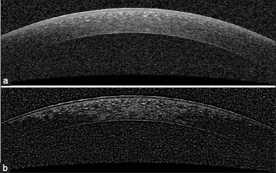
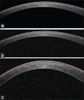
In this paper, we segment the boundaries of corneal layers by utilizing Gaussian mixture model (GMM) method. Our method segments three important corneal boundaries in OCT images. These layers are as follows: Epithelium, Bowman and endothelium. The OCT images captured from high-tech devices may have high SNR [Figure 1a], but in many cases, they have a low-SNR [Figure 1b]. Furthermore, some of OCT images may be affected by different types of artifact like central artifact. The central artifact is the vertical saturation artifact that occurs around the center of the cornea due to the back-reflections from the corneal apex, which saturates the spectrometer line camera.[29] The data used in this work is taken from Heidelberg OCT-spectralis HRA imaging system in Noor Ophthalmology Center in Tehran, Iran. The high-quality of images taken from this system guarantees that we have no central artifact. The paper is organized as follows: section 2 describes the theory of GMM. Section 3 discusses the segmentation method of the mentioned corneal layers by utilizing GMM algorithm. Section 4 compares the results of this method against the corneal specialist manual segmentation and the conclusion is discussed in section 5.

Figure 1.

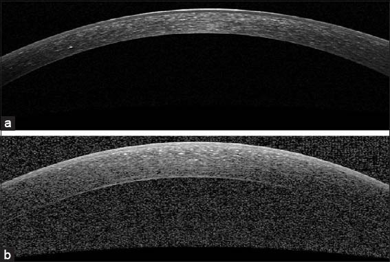
Examples of corneal images of varying signal-to-noise ratio (SNR) used in this study. (a) A high SNR corneal image. (b) A low-SNR corneal image

GMM

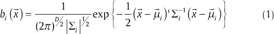
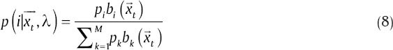
Kim and Kang[38] explained that GMM is a method to estimate the probability density function (PDF) using a combination of Gaussian functions. The elements of mixtures are defined as D-dimensional Gaussians and the equation of a D-dimensional Gaussian distribution is given below:

where is a D.dimensional vector of features of the input image, is the mean vector and is the covariance matrix. A weighted mixture of M Gaussian distribution is given in the equation below:

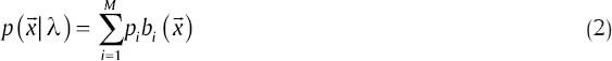
where p_is are the weights of mixture elements and:

μi, pi and Σ_i are parameters of GMM and we show this model with λ. We formulate GMM as a maximum likelihood problem and estimate its parameters by utilizing expectation-maximization (EM) algorithm. EM algorithm starts from an initial λ and estimates the new one as:

This procedure is repeated until converging to a good model. The number of EM iterations can be control by selecting a threshold. One way to select a threshold is that, GMM going on until the difference between and p(x|λ) be smaller than a value or we can directly choose the number of EM iterations as an input for GMM. We use the following equations in each iteration of EM algorithm to estimate the parameters (for T training vectors):

In fact, EM algorithm reaches its goal during two steps: Expectation step (E) and maximization step (M). Step E corrects the PDF and step M maximize it in each iteration. is the posterior probability for class i in step E and is defined as below:

As mentioned, is a D-dimensional vector of features of the input image. Various features can be considered for the image like pixel location for 3D plots, RGB space of the image, Luv space of the image and Lab space of the image.

GMM is an automatic method to segment an image based on its statistical properties. This method fits a number of Gaussian functions to the distribution of the image. Since our images often have the same distribution, it can show a good performance in our work. In this way that we can localize the object in the next image by tracking its distribution. GMM has also been used in OCT image processing by.[39,40] Furthermore, this method has also been utilized in segmentation of fluorescein angiograms in.[41] So we can say that GMM is capable for segmentation in our work.

THE PROPOSED METHOD

Epithelium, Bowman and endothelium are three important corneal layers [Figure 2].

Figure 2.

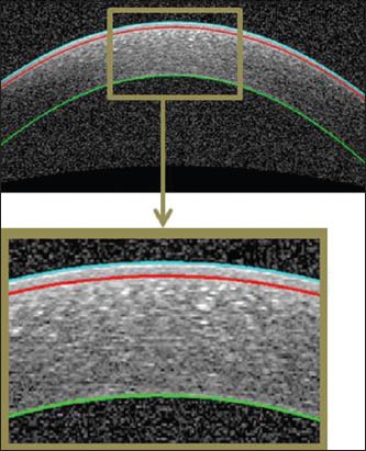
An example of segmented corneal image. The epithelium boundary (cyan), the Bowman boundary (red), and the endothelium boundary (green)

In this section, the proposed method for segmenting the boundaries of epithelium, Bowman and endothelium layers are explained. At first, the method for segmentation of the boundaries of epithelium and endothelium layers is explained. Then we elaborate how to extrapolate the curves to low-SNR regions. Then, segmenting the boundary of Bowman layer and contrast enhancement of the Bowman boundary is described in the last part of this section.

Segmenting the Boundaries of Epithelium and Endothelium Layers

To obtain these two boundaries, we first apply a low-pass filter through a (1 × 30) Gaussian kernel (sigma of 10) to minimize the effect of noise [Figure 3a]. The selected kernel size leads to uniformity of the image noise and prevents from segmentation of whatever has been affected by noise (as a distinct element). Then we give the denoised image to the GMM algorithm and determine the number of classes to be two. The final result of GMM [Figure 3b] shows the approximate location of these two boundaries. As it can be seen in Figure 3c, the detected boundary is not exactly on the border of epithelium. To overcome this problem, we can use the horizontal gradient of the original image and with the help of the current boundary, we look for the lowest gradient in a small neighborhood [Figure 4].

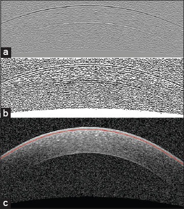
Figure 3.

Segmentation of epithelium and endothelium boundaries. (a) Reducing the speckle noise with a Gaussian low-pass filter. This image is used as an input for Gaussian mixture model (GMM). (b) GMM output. This is the image which is used for segmentation of desirable boundaries. (c) Segmentation result (before correction)

Figure 4.

Epithelium boundary after correction

Extrapolation to Low SNR Regions

Some images have low-SNR areas in two peripheral regions and the obtained boundaries in these regions are not accurate enough. Therefore, we localize the low-SNR regions and extrapolate the central curve in such areas. For this purpose, we use the second derivative of endothelium boundary [Figure 5a] and search around the middle of this vector to find values below zero. It indicates that there is a positive inflection in the second derivative, which should not occur for normal cornea. The location of this positive inflection reveals the low-SNR areas of the image. In this step, a parabolic curve can be fitted to the estimated boundary with finding the coefficients of polynomial of degree 4 for the correct estimated border, in a least squares sense. Suppose that we have m pairs of data:

Figure 5.

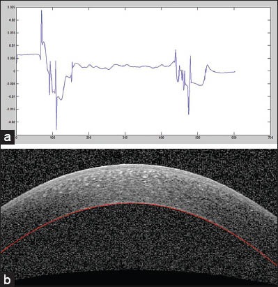
Extrapolation to low-signal-to-noise ratio (SNR) regions. (a) The second derivative plot of endothelium layer boundary to detect low-SNR regions of this boundary. (b) Extrapolation result

(x_i,y_i), i = 1,…, m

Consider the fit function with three basic functions:

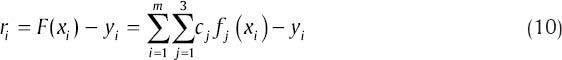
The objective is to find the c_j such that F(x) ≈ y_i. Since F(x) ≠ y_i, the residual for each data point is:

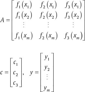
The least square solution gives the c_j that minimize ‖ r ‖₂. The over determined system is as below:

where

The least squares method provides the compromise solution that minimizes 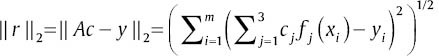. The c that minimizes ‖ r ‖₂ satisfies the normal equations:

As mentioned above, we can recognize the starting points of the low-SNR regions using second derivative and extrapolation will be done using a degree 4 polynomial [Figure 5b]. To create smooth junctions in the final boundary, smoothing operators can then be used. For this purpose, a local regression using weighted linear least squares that assigns lower weight to outliers can be used. To find low-SNR regions for epithelium, we use the unsigned second derivative of epithelium boundary and search for values greater than a threshold. This threshold is 0.0045 and the value is determined based on trial and error.

Segmenting the Boundary of Bowman Layer

For this purpose, we first enhance this boundary because in most cases it is very weak.

Contrast Enhancement to have Detectable Bowman Boundary

For this purpose, we modified a method proposed by Esmaeili et al.[42] This algorithm corrects non-uniform background and increases the contrast of Bowman boundary in Figure 6a. During this process each pixel f (i, j) of the image is adjusted as follows:

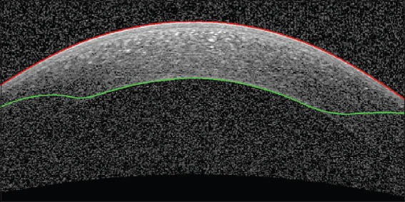
Figure 6.

Contrast enhancement of original image for segmentation of Bowman boundary. (a) Original image. (b) The enhanced image

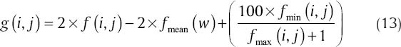
where f_mean, f_min (i, j) and f_max (i, j) are, respectively, the mean, minimum and maximum intensity values of the image within a window W of size 10 × 10 [Figure 6b].

After enhancement, we obtain the horizontal edge response to Sobel gradient of the enhanced image. We use this image as an input of GMM because in this case, the layer distinguishes itself from other parts of the image [Figure 7a]. Figure 7b is the output of GMM and using this image we can localize the Bowman boundary. Since we have obtained the epithelium boundary (as described in Epithelium and Endothelium segmentation part), the Bowman boundary is achievable by tracing epithelium toward down to get a white to black change in brightness. The middle of the Bowman boundary will be detected exactly, but the periphery may be affected by the noise and would create outliers. To overcome this problem, we find the outliers like previously mentioned method for low-SNR areas in epithelium, and then extrapolate the curve to the outside of these points. The result is shown in Figure 7c.

Figure 7.

Segmentation of Bowman layer boundary. (a) Horizontal gradient of the enhanced image. (b) Gaussian mixture model output to the input of (a). (c) Segmentation result

EXPERIMENTAL RESULTS

In this study, we used corneal OCT images taken from 10 normal subjects. Each subject includes 40 slices of the whole cornea. The algorithm is tested on images taken from Heidelberg OCT-spectralis HRA imaging system in Noor Ophthalmology Center in Tehran, Iran. This system has a pre-processing stage. To evaluate the robustness and accuracy of the proposed algorithm, we use manual segmentation by two corneal specialists. For this purpose, 20 images selected randomly from all subjects. We calculated the unsigned and signed error of this algorithm against manual results.

The boundaries were segmented automatically using a MATLAB (R2011a) implementation of our algorithm. A computer with Microsoft Windows 7 x32 edition, Intel Core i5 central processing unit at 2.5 GHz, 6 GB random access memory was used for the processing. The average computation time was 7.99 s/image. The mean and standard deviation of unsigned and signed error were calculated and are shown in Tables 1 and 2, respectively. The mean and standard deviation of unsigned error is defined as follows:

Table 1.

Mean and SD of unsigned error in corneal layer boundary segmentation between automatic and manual results and among two corneal specialists

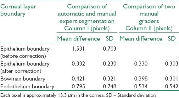
Table 2.

Mean and SD of signed error in corneal layer boundary segmentation between automatic and manual segmentation and among two corneal specialists

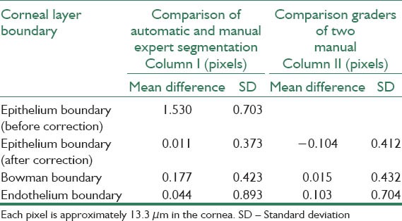
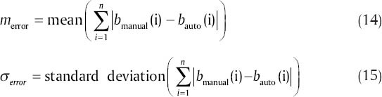
where m_error and σ_error are the mean and standard deviation of unsigned error between manual and automatic method, n is the number of points to calculate the layer error (width of the image), b_manual and bauto are the boundary layers which are obtained manually and automatically, respectively. The mean value of manual segmentation by two independent corneal specialists is considered as b_manual in above equations and the inter-observer errors are also provided in Tables 1 and 2. The direct comparison of these values with the reported errors shows that the performance of the algorithm is acceptable in comparison with manual segmentation. Furthermore, the visual results of automatic segmentation of the corneal layers using proposed algorithm in this study for sample images are shown in Figure 8.

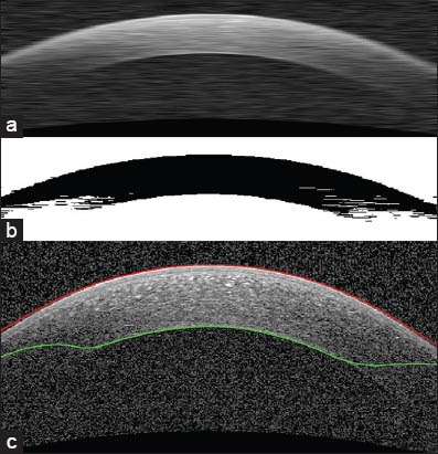
Figure 8.

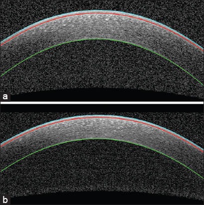
Examples of segmented corneal images, in which the cyan curve is the epithelium boundary, the red curve is Bowman boundary, and the green curve is the endothelium boundary

According to the possibility of comparing our results with other methods, it should be mentioned that the only available dataset for corneal OCT is provided by.[29] Unfortunately, the images in[29] have single Gaussian distribution [Figure 9] and the proposed method is based on classification by GMM method (which needs multiple Gaussians). Therefore, the proposed method is not able to classify these images correctly.

Figure 9.

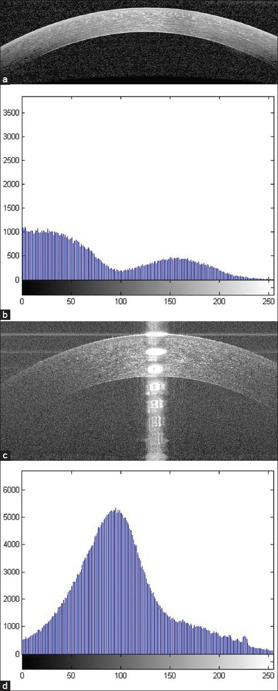
(a) An example of corneal optical coherence tomography (OCT) image used in our work. (b) The histogram of (a) which includes multiple Gaussians. (c) An example of corneal OCT image used by Larocca et al (d) The histogram of (c) which includes a single Gaussian distribution

To demonstrate the robustness of our algorithm against noise, we chose a raw image and add a Gaussian white noise with zero mean and variance as below:

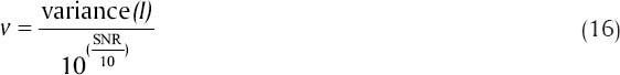
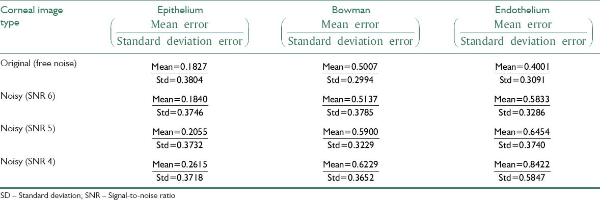
where v is the Gaussian white noise variance and I is the normalized image. We use MATLAB toolbox and imnoise command to add noise with three different SNRs to the image. It should be considered that we don’t have any ideal or noise less image and we can only compare our results in the presence of more added noise. Figure 10a and b shows the original image and its noisy image with SNR 4, respectively. Figure 10c shows the layers which obtained for the noisy image with SNR 4. The mean and standard deviation of unsigned and signed error for three different SNRs were calculated and are shown in Tables 3 and 4. As can be observed there are minimum differences from the obtained error between the noisy images and the original image that demonstrate the robustness of our algorithm against noise.

Figure 10.

Evaluation of the noise effect on the segmentation of the boundaries of corneal layers. (a) The original image of cornea which is high signal-to-noise ratio (SNR) (raw image). (b) The noisy image of (a) with SNR 4. (c) The boundaries of cornea which is shown in (b)

Table 3.

Mean and SD of unsigned error for the original and its noisy images with different SNRs

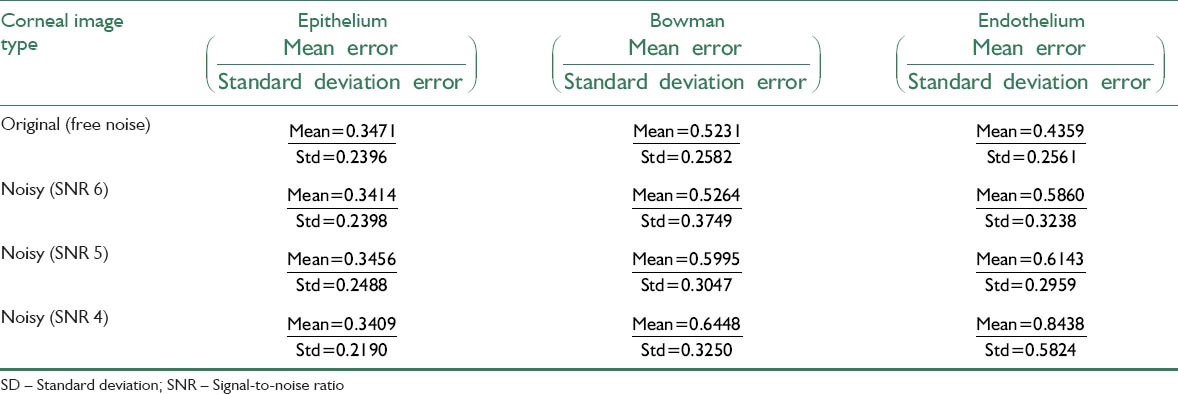
Table 4.

Mean and standard deviation of signed error for the original and its noisy images with different SNRs

CONCLUSION AND FUTURE WORK

In this paper, we proposed an automatic method for segmentation of three important corneal layers of normal eyes using OCT devices. Our approach has a good performance in noisy images and is accurate in low-SNR regions. The obtained results are very close to the results of the specialists.

The large volume of corneal images in the clinics makes manual segmentation time-consuming impractical and subjective. However, the proposed method does not require any user interaction, saves time and produces accurate boundary tracing.

In this paper the standard form of GMM was used for segmentation. More accurate GMMs which are able to better capture the statistical properties of data (such as proposed mixture model in[43] which employs a local bivariate circular symmetric Laplacian mixture model) can improve the results, also may result in removing the noise reduction step in our algorithm by proposing the noise in the initial mixture model of OCT data.

The 3D analysis can be a valuable step to evaluate changes in corneal volume, as future work.

BIOGRAPHIES

Mahdi Kazemian Jahromi received the B.S. degree from Azad university of jahrom, Iran, in 2011 in communication Engineering, and the M.S. degree from the Isfahan University of Medical Sciences, Iran, in 2014 in biomedical engineering. His research interests are in biomedical image Processing and computer vision.

E.mail: mahdi_kazemian71@yahoo.com

Raheleh Kafieh received the B.S. degree from Sahand University of Technology, Iran, in 2005 and the M.S. degree from the Isfahan University of Medical Sciences, Iran, in 2008, both in biomedical engineering. She is currently working toward the Ph.D. degree at the Department of Biomedical Engineering, Isfahan University of Medical Sciences. Her research interests are in biomedical image processing, computer vision, graph algorithms, and sparse transforms. She is a student member of the IEEE and the IEEE Signal Processing Society.

E.mail: r_kafieh@yahoo.com

Hossein Rabbani received the B.Sc. degree in electrical engineering (communications) from Isfahan University of Technology, Isfahan, Iran, in 2000 with the highest honors, and the M.Sc. and Ph.D. degrees in bioelectrical engineering from Amirkabir University of Technology (Tehran Polytechnic), Tehran, Iran, in 2002 and 2008, respectively. In 2007, he was with the Department of Electrical and Computer Engineering, Queen's University, Kingston, ON, Canada, as a Visiting Researcher, and in 2011 with the Iowa University, IA, USA, as a Postdoctoral Research Scholar. He is now an Associate Professor in Biomedical Engineering Department and Medical Image and Signal Processing Research Center, Isfahan University of Medical Sciences, Isfahan. His main research interests are medical image analysis and modeling, statistical (multidimensional) signal processing, sparse transforms, and image restoration.

E.mail: h_rabbani@med.mui.ac.ir

Alireza Mehri Dehnavi was born in Isfahan province at 1961. He had educated in Electronic Engineering at Isfahan University of Technology at 1988. He had finished Master of Engineering in Measurement and Instrumentation at Indian Institute of Technology Roorkee (IIT Roorkee) in India at 1992. He has finished his PhD in Medical Engineering at Liverpool University in UK at 1996. He is an Associate Professor of Medical Engineering at Medical Physics and Engineering Department in Medical School of Isfahan University of Medical Sciences. He is currently visiting at School of Optometry and Visual Science at University of Waterloo in Canada. His research interests are medical optics, devices and signal processing.

E.mail: mehri@med.mui.ac.ir

Alireza Peyman was born in Tabriz at 1974. He is an ophthalmologist (fellowship of cornea and anterior segment), and fulltime faculty member (assistant professor) in Isfahan University of Medical Sciences, Iran.

E.mail: peyman@med.mui.ac.ir

Fedra Hajizadeh received the M.D. degree from Tehran University of Medical Sciences, Tehran, Iran, in 1995 and completed the Ophthalmology Residency and VitreoRetinal Fellowship both at Farabi Eye Hospital of Tehran University of Medical Sciences in 1999 and 2004, respectively. Since 2008, she has been a Consulting Surgeon of VitreoRetinal diseases and Research Scientist at Noor Eye Hospital, Tehran, Iran and now in the same hospital she is working in Retinal Imaging Center. Her current research includes optical coherence tomography (OCT) of retina, ocular trauma, and retinal fluorescein angiography. Dr. Hajizadeh received the Honorable Mention award at the Ophthalmic Photographers Society Exhibit, ASCRS.ASOASymposium and Congress, Chicago, Illinois, USA, April 2012.

E.mail: fhajizadeh@noorvision.com

Mohammadreza Ommani received the B.Sc. degree in electrical engineering from Isfahan University of Technology, Isfahan, Iran, in 2000. He is already an expert of biomedical engineering in Iranian Association Official Experts and Managing Director of Pooya Did Parto company that focuses on Ophthalmic devices. He is currently working on calibration and installation of ophthalmic instruments and has certificates from Carl Ziess Meditc, Heidelberg, Optovue and many other companies. His research interests include OCT, Angiography and medical.

E.mail: mohammadommani@yahoo.com

REFERENCES

- 1.Chiu SJ, Li XT, Nicholas P, Toth CA, Izatt JA, Farsiu S. Automatic segmentation of seven retinal layers in SDOCT images congruent with expert manual segmentation. Opt Express. 2010;18:19413–28. doi: 10.1364/OE.18.019413. [DOI] [PMC free article] [PubMed] [Google Scholar]
- 2.Fujimoto JG, Drexler W, Schuman JS, Hitzenberger CK. Optical coherence tomography (OCT) in ophthalmology: Introduction. Opt Express. 2009;17:3978–9. doi: 10.1364/oe.17.003978. [DOI] [PMC free article] [PubMed] [Google Scholar]
- 3.Garvin MK, Abràmoff MD, Wu X, Russell SR, Burns TL, Sonka M. Automated 3-D intraretinal layer segmentation of macular spectral-domain optical coherence tomography images. IEEE Trans Med Imaging. 2009;28:1436–47. doi: 10.1109/TMI.2009.2016958. [DOI] [PMC free article] [PubMed] [Google Scholar]
- 4.Haeker M, Sonka M, Kardon R, Shah VA, Wu X, Abràmoff MD, editors. Automated segmentation of intraretinal layers from macular optical coherence tomography images. Proc SPIE. 2007 [Google Scholar]
- 5.Huang D, Swanson EA, Lin CP, Schuman JS, Stinson WG, Chang W, et al. Optical coherence tomography. Science. 1991;254:1178–81. doi: 10.1126/science.1957169. [DOI] [PMC free article] [PubMed] [Google Scholar]
- 6.Lee K, Niemeijer M, Garvin MK, Kwon YH, Sonka M, Abramoff MD. Segmentation of the optic disc in 3-D OCT scans of the optic nerve head. IEEE Trans Med Imaging. 2010;29:159–68. doi: 10.1109/TMI.2009.2031324. [DOI] [PMC free article] [PubMed] [Google Scholar]
- 7.Schuman SG, Koreishi AF, Farsiu S, Jung SH, Izatt JA, Toth CA. Photoreceptor layer thinning over drusen in eyes with age-related macular degeneration imaged in vivo with spectral-domain optical coherence tomography. Ophthalmology. 2009;116:488–4962. doi: 10.1016/j.ophtha.2008.10.006. [DOI] [PMC free article] [PubMed] [Google Scholar]
- 8.Tolliver D, Koutis I, Ishikawa H, Schuman J, Miller G, editors. Automatic multiple retinal layer segmentation in spectral domain oct scans via spectral rounding. ARVO Annual Meeting. 2008 [Google Scholar]
- 9.Herndon LW, Choudhri SA, Cox T, Damji KF, Shields MB, Allingham RR. Central corneal thickness in normal, glaucomatous, and ocular hypertensive eyes. Arch Ophthalmol. 1997;115:1137–41. doi: 10.1001/archopht.1997.01100160307007. [DOI] [PubMed] [Google Scholar]
- 10.Izatt JA, Hee MR, Swanson EA, Lin CP, Huang D, Schuman JS, et al. Micrometer-scale resolution imaging of the anterior eye in vivo with optical coherence tomography. Arch Ophthalmol. 1994;112:1584–9. doi: 10.1001/archopht.1994.01090240090031. [DOI] [PubMed] [Google Scholar]
- 11.Kohlhaas M, Boehm AG, Spoerl E, Pürsten A, Grein HJ, Pillunat LE. Effect of central corneal thickness, corneal curvature, and axial length on applanation tonometry. Arch Ophthalmol. 2006;124:471–6. doi: 10.1001/archopht.124.4.471. [DOI] [PubMed] [Google Scholar]
- 12.Li HF, Petroll WM, Møller-Pedersen T, Maurer JK, Cavanagh HD, Jester JV. Epithelial and corneal thickness measurements by in vivo confocal microscopy through focusing (CMTF) Curr Eye Res. 1997;16:214–21. doi: 10.1076/ceyr.16.3.214.15412. [DOI] [PubMed] [Google Scholar]
- 13.Liu Z, Huang AJ, Pflugfelder SC. Evaluation of corneal thickness and topography in normal eyes using the Orbscan corneal topography system. Br J Ophthalmol. 1999;83:774–8. doi: 10.1136/bjo.83.7.774. [DOI] [PMC free article] [PubMed] [Google Scholar]
- 14.Liu Z, Pflugfelder SC. The effects of long-term contact lens wear on corneal thickness, curvature, and surface regularity. Ophthalmology. 2000;107:105–11. doi: 10.1016/s0161-6420(99)00027-5. [DOI] [PubMed] [Google Scholar]
- 15.Morad Y, Sharon E, Hefetz L, Nemet P. Corneal thickness and curvature in normal-tension glaucoma. Am J Ophthalmol. 1998;125:164–8. doi: 10.1016/s0002-9394(99)80086-5. [DOI] [PubMed] [Google Scholar]
- 16.Müller LJ, Pels E, Vrensen GF. The specific architecture of the anterior stroma accounts for maintenance of corneal curvature. Br J Ophthalmol. 2001;85:437–43. doi: 10.1136/bjo.85.4.437. [DOI] [PMC free article] [PubMed] [Google Scholar]
- 17.Radhakrishnan S, Rollins AM, Roth JE, Yazdanfar S, Westphal V, Bardenstein DS, et al. Real-time optical coherence tomography of the anterior segment at 1310 nm. Arch Ophthalmol. 2001;119:1179–85. doi: 10.1001/archopht.119.8.1179. [DOI] [PubMed] [Google Scholar]
- 18.Reinstein DZ, Archer TJ, Gobbe M, Silverman RH, Coleman DJ. Epithelial thickness in the normal cornea: Three-dimensional display with Artemis very high-frequency digital ultrasound. J Refract Surg. 2008;24:571–81. doi: 10.3928/1081597X-20080601-05. [DOI] [PMC free article] [PubMed] [Google Scholar]
- 19.Reinstein DZ, Silverman RH, Rondeau MJ, Coleman DJ. Epithelial and corneal thickness measurements by high-frequency ultrasound digital signal processing. Ophthalmology. 1994;101:140–6. doi: 10.1016/s0161-6420(94)31373-x. [DOI] [PubMed] [Google Scholar]
- 20.Seitz B, Torres F, Langenbucher A, Behrens A, Suárez E. Posterior corneal curvature changes after myopic laser in situ keratomileusis. Ophthalmology. 2001;108:666–72. doi: 10.1016/s0161-6420(00)00581-9. [DOI] [PubMed] [Google Scholar]
- 21.Shimmyo M, Ross AJ, Moy A, Mostafavi R. Intraocular pressure, Goldmann applanation tension, corneal thickness, and corneal curvature in Caucasians, Asians, Hispanics, and African Americans. Am J Ophthalmol. 2003;136:603–13. doi: 10.1016/s0002-9394(03)00424-0. [DOI] [PubMed] [Google Scholar]
- 22.Danesh H, Kafieh R, Rabbani H, Hajizadeh F. Segmentation of choroidal boundary in enhanced depth imaging OCTs using a multiresolution texture based modeling in graph cuts. Comput Math Methods Med 2014. 2014:1–9. doi: 10.1155/2014/479268. [DOI] [PMC free article] [PubMed] [Google Scholar]
- 23.Graglia F, Mari JL, Baikoff G, Sequeira J, editors. Contour detection of the cornea from OCT radial images. Engineering in Medicine and Biology Society, 2007 EMBS 2007 29th Annual International Conference of the IEEE. IEEE. 2007 doi: 10.1109/IEMBS.2007.4353619. [DOI] [PubMed] [Google Scholar]
- 24.Kafieh R, Rabbani H, Abramoff M, Sonka M, editors. Intra-retinal layer segmentation of optical coherence tomography using diffusion map. Acoustics, Speech and Signal Processing (ICASSP) 2013. IEEE International Conference on: IEEE. 2013 [Google Scholar]
- 25.Kafieh R, Rabbani H, Abramoff MD, Sonka M. Intra-retinal layer segmentation of 3D optical coherence tomography using coarse grained diffusion map. Med Image Anal. 2013;17:907–28. doi: 10.1016/j.media.2013.05.006. [DOI] [PMC free article] [PubMed] [Google Scholar]
- 26.Kafieh R, Rabbani H, Hajizadeh F, Ommani M, Kermani S. An accurate multimodal 3D vessel segmentation method based on brightness variations on OCT layers and curvelet domain fundus image analysis. IEEE Trans Biomed Eng. 2013;60:2815–23. doi: 10.1109/TBME.2013.2263844. [DOI] [PubMed] [Google Scholar]
- 27.Kafieh R, Rabbani H, Kermani S. A review of algorithms for segmentation of optical coherence tomography from retina. J Med Signals Sens. 2013;3:45–60. [PMC free article] [PubMed] [Google Scholar]
- 28.Kajić V, Povazay B, Hermann B, Hofer B, Marshall D, Rosin PL, et al. Robust segmentation of intraretinal layers in the normal human fovea using a novel statistical model based on texture and shape analysis. Opt Express. 2010;18:14730–44. doi: 10.1364/OE.18.014730. [DOI] [PubMed] [Google Scholar]
- 29.Larocca F, Chiu SJ, McNabb RP, Kuo AN, Izatt JA, Farsiu S. Robust automatic segmentation of corneal layer boundaries in SDOCT images using graph theory and dynamic programming. Biomed Opt Express. 2011;2:1524–38. doi: 10.1364/BOE.2.001524. [DOI] [PMC free article] [PubMed] [Google Scholar]
- 30.Rabbani H, Sonka M, Abramoff MD. Optical Coherence tomography noise reduction using anisotropic local bivariate Gaussian mixture prior in 3D complex wavelet domain. Int J Biomed Imaging 2013. 2013:417491. doi: 10.1155/2013/417491. [DOI] [PMC free article] [PubMed] [Google Scholar]
- 31.Gora M, Karnowski K, Szkulmowski M, Kaluzny BJ, Huber R, Kowalczyk A, et al. Ultra high-speed swept source OCT imaging of the anterior segment of human eye at 200 kHz with adjustable imaging range. Opt Express. 2009;17:14880–94. doi: 10.1364/oe.17.014880. [DOI] [PubMed] [Google Scholar]
- 32.DelMonte DW, Kim T. Anatomy and physiology of the cornea. J Cataract Refract Surg. 2011;37:588–98. doi: 10.1016/j.jcrs.2010.12.037. [DOI] [PubMed] [Google Scholar]
- 33.Eichel JA, Mishra AK, Clausi D, Fieguth P, Bizheva KK, editors. A novel algorithm for extraction of the layers of the cornea. Computer and Robot Vision, 2009 CRV’09 Canadian Conference on: IEEE. 2009 [Google Scholar]
- 34.Li Y, Netto MV, Shekhar R, Krueger RR, Huang D. A longitudinal study of LASIK flap and stromal thickness with high-speed optical coherence tomography. Ophthalmology. 2007;114:1124–32. doi: 10.1016/j.ophtha.2006.09.031. [DOI] [PubMed] [Google Scholar]
- 35.Li Y, Shekhar R, Huang D, editors. Segmentation of 830- and 1310-nm LASIK corneal optical coherence tomography images [4684-18]. Proceedings-SPIE The International Society for Optical Engineering; 2002. International Society for Optical Engineering. 1999 [Google Scholar]
- 36.Li Y, Shekhar R, Huang D. Corneal pachymetry mapping with high-speed optical coherence tomography. Ophthalmology. 2006;113:792–92. doi: 10.1016/j.ophtha.2006.01.048. [DOI] [PMC free article] [PubMed] [Google Scholar]
- 37.Hutchings N, Simpson TL, Hyun C, Moayed AA, Hariri S, Sorbara L, et al. Swelling of the human cornea revealed by high-speed, ultrahigh-resolution optical coherence tomography. Invest Ophthalmol Vis Sci. 2010;51:4579–84. doi: 10.1167/iovs.09-4676. [DOI] [PubMed] [Google Scholar]
- 38.Kim SC, Kang TJ. Texture classification and segmentation using wavelet packet frame and Gaussian mixture model. Pattern Recognit. 2007;40:1207–21. [Google Scholar]
- 39.Cha YM, Han JH. High-accuracy retinal layer segmentation for optical coherence tomography using tracking kernels based on the Gaussian mixture model. IEEE Journal of Selected Topics in Quantum Electronics. 2013;20:29. [Google Scholar]
- 40.Cha YM, Han JH, editors. Efficient edge detection method for anatomic feature extraction of neuro-sensory tissue image based on optical coherence tomography. Brain-Computer Interface (BCI), 2013. International Winter Workshop on: IEEE. 2013 [Google Scholar]
- 41.El-Shahawy MS, ElAntably A, Fawzy N, Samir K, Hunter M, Fahmy AS, editors. Segmentation of diabetic macular edema in fluorescein angiograms. Biomedical Imaging: From Nano to Macro, 2011. IEEE International Symposium on: IEEE. 2011 [Google Scholar]
- 42.Esmaeili M, Rabbani H, Dehnavi A, Dehghani A. Automatic detection of exudates and optic disk in retinal images using curvelet transform. IET Image Process. 2012;6:1005–13. [Google Scholar]
- 43.Rabbani H, Vafadust M, Selesnick I, Gazor S. Image Denoising Employing a Mixture of Circular Symmetric Laplacian Models with Local Parameters in Complex Wavelet Domain, Acoustics, Speech and Signal Processing, 2007. ICASSP 2007. IEEE International Conference. 2007 Apr 15-20;1:I-805–I-808. [Google Scholar]