

Abstract
In this article we will discuss the integration of developmental patterning mechanisms with waves of competency that control the ability of a homogeneous field of cells to react to pattern forming cues and generate spatially heterogeneous patterns. We base our discussion around two well known patterning events that take place in the early embryo: somitogenesis and feather bud formation. We outline mathematical models to describe each patterning mechanism, present the results of numerical simulations and discuss the validity of each model in relation to our example patterning processes.
Keywords: Developmental waves, Patterning mechanisms, Mathematical modelling, Somitogenesis, Feather bud formation
1 Introduction
Complex patterns arise as organisms grow, develop and interact with their environment. Be it a spatially heterogeneous distribution of cell types, density or gene expression, there are a plethora of examples of pattern formation in the early embryo, from Drosophila segmentation (Gilbert, 2006, Sanson, 2001) to digit formation and limb chrondrogenesis (Tickle, 2000, Tickle, 2006), subdivision of the vertebrate antero-posterior (AP) axis into somites (Gossler and Hrabé de Angelis, 1998, Pourquié, 2001b) and formation of the avian integument (Yu et al., 2002, Yu et al., 2004). In spite of the dramatic advances made in genetic and molecular biology, we are still looking for answers to fundamental questions: in particular, what are the underlying mechanisms that give rise to patterning in development?
Developmental biologists have shown that graded distributions of morphogens play important roles in pattern specification and generation (Green and Smith, 1991, Murray et al., 1988, Tabata and Takei, 2004, Wolpert et al., 2006). However, there are still many unanswered questions as to: how these patterns are specified; how morphological changes take place; how patterns are regulated; and how the underlying mechanisms display robustness to intrinsic and environmental perturbations.
Wolpert proposed a mechanism for providing positional information via a morphogen gradient with his French Flag model (Wolpert, 1969). In the model, each cell in a line of cells has the potential to be either blue, white or red. The line of cells is exposed to a concentration profile of a morphogen and each cell interprets the information from the concentration profile by varying its response to different concentration thresholds of morphogen: cells become blue, white or red according to their interpretation of the information. In general, it is accepted that Wolpert's definition implies at least two thresholds of morphogen concentration, or the division of the field into at least three different states.
In the majority of applications of this model, it is supposed that the gradient is fixed or the morphogen concentration evolves towards a stationary gradient, so cells differentiate according to their position within the field and the functional role of the gradient is to provide spatial information. However, there are patterning events observed in biological systems in which the gradient is not stationary: rather, it travels across the tissue in a wave-like fashion, conferring, as it passes, some degree of determination (Dubrulle et al., 2001, Lin et al., 2006). Typically this kind of gradient acts in an all-or-nothing manner with a single threshold: above threshold concentration, cells remain in an immature state and have no pattern forming ability; below threshold concentration they are competent to form patterning structures. Thus, in this case, the wave may control both spatial and temporal aspects of development.
It is this latter case that we will discuss here, both in relation to pattern specification and morphological events. How may a wave of competence combine with a local patterning mechanism to control the spatio-temporal patterns visualised in the embryo? Our studies are motivated by two paradigms from developmental biology: (i) somitogenesis (segmentation of the AP axis of vertebrate embryos) and (ii) formation of the avian integument. We begin by outlining the main events involved in each process, in the context of waves and patterning. Next we introduce several well-known mathematical models for pattern formation, discuss their application to our biological examples and the role of waves in controlling pattern forming ability. We conclude with a short discussion: comparing and contrasting each model and its validity in the light of current experimental knowledge. Finally, we remark upon the new challenges that interdisciplinary modelling in this area has brought about.
1.1 Somitogenesis
Somites are tightly bound groups of cells that lie along the AP axis of vertebrate embryos. They are transient structures and further differentiation of the somites gives rise to the vertebrae, ribs and other associated features of the trunk (Gossler and Hrabé de Angelis, 1998). Somitogenesis is tightly regulated in both space and time (Pourquié, 2003a), with each somite forming from a seemingly uniform field of cells via a mechanism that involves the interaction of a moving gradient of morphogen and a segmentation clock.
Somites form from the pre-somitic mesoderm (PSM), thick bands of tissue that lie along the AP axis. At regular time intervals (every 90 minutes in the chick), groups of cells in the anterior PSM undergo changes in their adhesive and migratory behaviour and condense together to form an epithelial block of cells known as a somite. In this way, somites form in a very strict AP sequence (Gossler and Hrabé de Angelis, 1998, Stickney and Devoto, 2000, Stockdale et al., 2000) and the budding of cells from the anterior end of the PSM compensates for the addition of cells at the posterior end of the PSM as the body axis lengthens. Each band of the PSM stays approximately constant in length throughout the process of segmentation and a wave of cell determination appears to sweep along the AP axis leaving somites in its wake (Baker et al., 2008, Schnell and Maini, 2000, Schnell et al., 2002).
Several genes are expressed dynamically in the PSM with cycling times equal to the time taken to form one somite (Déqueant et al., 2006). For example, gene expression bands of c-hairy1 (Palmeirim et al., 1997) and l-fng (McGrew and Pourquié, 1998) sweep along the PSM in a posterior to anterior direction coming to rest in the newly forming somites. Expression is considered to arise as a result of a segmentation clock acting within PSM cells (Pourquié, 2001a).
Another gene with dynamic expression in the PSM is fgf8. A gradient of fgf8 signalling exists along the AP axis, with elevated levels in the posterior PSM gradually decreasing with movement in an anterior direction (Dubrulle et al., 2001, Dubrulle and Pourquié, 2002). This gradient is mirrored by an opposing gradient of retinoic acid (see (Diez del Corral et al., 2002, Diez del Corral et al., 2003, Diez del Corral and Storey, 2004) and Figure 1 for more details). As the axis elongates posteriorly and somites form anteriorly, the wavefront of FGF8 moves in a posterior direction along with the tail, so that the FGF8 gradient stays in a constant position relative to the PSM throughout somite formation. Hence cells are initially part of the region where FGF signalling prevails but as the gradient regresses they become part of the region where FGF signalling is virtually absent.
Figure 1. Schematic illustration of the vertebrate body plan during somitogenesis.

The top part of the diagram shows the opposing wavefronts of FGF8 and retinoic acid with the determination front (threshold level of FGF signalling) marked. The middle section of the diagram depicts the AP axis with several pairs of somites at the anterior end, followed by a sequence of five potential somite pairs, marked by a genetic pre-pattern, and the PSM. The bottom part of the diagram illustrates the interaction with the segmentation clock. The light blue blocks mark the position of the next somite pair to be specified: the posterior boundary is fixed by the level of the determination front at the time at which cells at the anterior boundary become able to signal.
Dubrulle and co-workers (Dubrulle et al., 2001, Dubrulle and Pourquié, 2002) have shown that the different levels of FGF8 in the posterior PSM coincide with regions of varying segmental determination and gene expression. In the posterior section cells are undetermined and plastic with respect to their future differentiation whilst in the anterior section cells are irreversibly committed to a particular developmental pathway (Dubrulle et al., 2001). The border which separates these regions is known as the determination front. It has been shown that down-regulation of FGF signalling is necessary for cells to be specified as somitic, and go on to form part of a somite. Figure 1 is an illustration of the vertebrate body plan during somitogenesis and the different regions of the PSM are clearly marked.
The first indications of somite patterning are observed as certain genes begin to exhibit striped expression patterns immediately anterior to the determination front (McGrew and Pourquié, 1998, Pourquié, 2001b, Pourquié, 2003b, Sawada et al., 2000). In mouse and zebrafish, members of the Mesp family are periodically activated, with expression initially occurring on a domain larger than a somite and subsequently narrowing to occupy the future posterior somite half (Saga et al., 2001, Sawada et al., 2000).
However, the first overt signs of somite formation arise as cells begin to condense – undergo changes in their adhesive and migratory properties – and continue later as they differentiate (Gossler and Hrabé de Angelis, 1998, Keynes and Stern, 1988). The aggregation process occurs in the anterior portion of the PSM and is triggered by the interactions of cell adhesion molecules (CAMs) on the surface membrane of somitic cells. Somite formation in avian and mouse embryos is preceded by compaction of the anterior region of PSM and a simultaneous increase in cadherin, N-CAM and N-cadherin expression (Duband et al., 1987, Kimura et al., 1995). Integrins also play an essential role in somite formation (Drake et al., 1992, Drake and Little, 1991). As a consequence it has been assumed that differential expression of adhesion molecules underlies the morphogenetic changes that take place during somite boundary formation (Murakami et al., 2006, Newman, 1993).
Experimental data show that the extracellular matrix (ECM) filaments have a reproducible morphogenic destiny that is characterised by directed transport (Czirok et al., 2004). Fibrillin 2 particles initially deposited in the PSM are translocated and eventually polymerise into an intricate scaffold of cables parallel to the AP axis. The cables coalesce near the midline before the appearance of the next-formed somite. This experimental evidence suggests that a direct translation from pre-pattern to coherent somites occurs via the changes in adhesive and migratory properties described previously.
There have been several models for somite formation and these have previously been reviewed by the authors (Baker et al., 2003, Baker et al., 2006a, Baker et al., 2008). In all but a single case (Schnell et al., 2002), the models specify only a pre-pattern for somitogenesis. The most recent models, both empirical and mathematical, are built upon a revised version of the clock and wavefront model which was first proposed by Cooke and Zeeman in 1976 (Cooke and Zeeman, 1976). The original model postulates the existence of a longitudinal positional information gradient along the AP axis of vertebrate embryos, which interacts with a smooth cellular oscillator (the clock) to set the time in each cell at which it will undergo a catastrophe. By catastophe, they mean a rapid change of state, which could possibly be the change in locomotory and adhesive behaviour of cells as they form somites.
With the discovery of a segmentation clock (Palmeirim et al., 1997, Pourquié, 2001a) and the wavefront of FGF8 travelling along the AP axis (Dubrulle et al., 2001, Dubrulle and Pourquié, 2004), Pourquié and co-workers proposed a revised clock and wavefront model; involving the interaction of clock and wavefront to gate cells into somites. For a cell at a particular point along the axis, they assume that competence to segment is achieved only when the level of FGF8 concentration falls below a certain threshold: the position of which defines the determination front (Dubrulle and Pourquié, 2002). In (Baker et al., 2006a, 2006b) we developed a mathematical formulation of this model and we refer readers to Appendix A for more details.
1.2 Feather germ formation
Feather buds, the precursors of the feathers, become visible shortly after fertilisation of the egg at about 6-9 days. Each bud consists of a thickening of the top layer of skin with an aggregation of mesenchymal cells from the second layer of skin lying beneath it. The epithelial cells making up the top layer of skin are unable to move, whereas the underlying mesenchymal cells are motile and can move around in the ECM (Wolpert, 1998). Feather buds form via the interaction of these layers; first, the epithelium over the tract (the feather forming region) becomes competent and then, via mechanisms mediated by cell adhesion and regulated by reaction-diffusion and competition, the cells migrate to form individual feather primordia (Jiang et al., 1999, Yu et al., 2002). See Figure 2 for more details of the feather bud formation process.
Figure 2. Schematic illustration of the processes involved in feather bud formation.
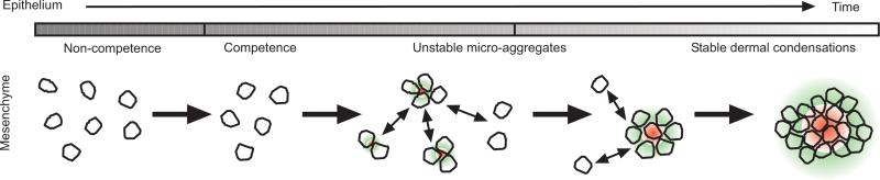
Initially the field is incompetent and cells cannot form buds. As a wave of competency passes, cells become able to form microaggregates and begin to secrete bud -promoting and -inhibiting factors. Promoting factors (red) recruit more cells into each aggregate whilst inhibiting factors (green) stop aggregates from becoming too large. Eventually, some aggregates are stabilised and go on to become dermal condensations. Adapted from (Lin et al., 2006).
The nature of the patterns formed is controlled by the presence of various activators and inhibitors which promote and suppress bud formation, and by the initial density of mesenchymal cells. Addition of promotors of bud formation, such as FGFs and Follistatin, increases bud density, whilst addition of inhibitors such as BMPs have the opposite effect (Jung et al., 1998, Widelitz et al., 1996). The final pattern of buds and interbuds can be overlain by a pattern of activators and inhibitors of bud and interbud formation (see Figure 2).
In vivo, feather buds first appear as dense regions on the skin surface; they develop in well defined lines and with a strict temporal ordering. The primary bud of each tract forms in the lumbar region at the level of the hindlimbs and patterning spreads bi-directionally along the midline axis. A wave of patterning then spreads out symmetrically and bilaterally from the midline (Jiang et al., 1999, Lin et al., 2006). Cells which lie initially in more lateral regions of the tract are unable to form feather buds until a wave of competency has passed (see Figure 2): although expression of β-catenin has been shown to be a reliable marker for competency, it is not clear what drives this morphogenetic wave (Lin et al., 2006).
Experimental techniques in vitro can be used to reset cells: embryonic chicken skin is dissected and the two skin layers are separated. With the mesenchymal cells dissociated from one another, the two layers are recombined. In this case, feather buds form simultaneously (Jiang et al., 2004), showing that the morphogenetic wave is not essential for patterning. The effects of perturbation of bud density can also be seen in vitro using a fixed size piece of epithelium and varying the initial density of mesenchymal cells. Below a certain threshold, there is a complete absence of buds, but as the initial density is increased, regularly-sized buds form, until maximal packing is achieved with a hexagonal arrangement (Jiang et al., 1999). Cell adhesion molecules have also been shown to play a role in pattern formation and their expression becomes progressively restricted to the feather buds as development proceeds (Jiang et al., 2004).
These results suggest that there are two mechanisms at work in vivo: a positional information gradient, which renders cells competent to form primordia, overlying a local patterning mechanism which is dependent on a number of activators, inhibitors, cell adhesion molecules and also upon cell density. However, it is not yet known whether the local patterning mechanism can be divided into two separate stages of pattern specification and cell differentiation/rearrangement, or whether the processes are intimately coupled.
2 Mathematical modelling in developmental biology
Mathematical modelling is now playing an increasingly important role in developmental biology: somitogenesis and avian appendage formation are two important paradigms for modelling in this field. Although still at an early stage, the experimental community is beginning to recognise that mathematical models allow one to put ideas and hypotheses into a concrete theoretical framework. Biological interactions and processes are often non-linear, and this is where intuitive, verbal reasoning may let us down: mathematical techniques allow us to analyse the effects of many interacting biological processes. Moreover, they allow us to direct research, discover/ask and even answer, pertinent questions and to design statistically sound and accurate experiments.
The impact of experimental perturbations, such as changes in the production and/or removal rates of a certain molecular constituent, can be mimicked in a mathematical model by changing, for example, certain parameter values. This is an important step in model validation: after one has verified that a model can display the results seen in wild type embryos, it is important to see whether it can display the behaviour observed when different model components are perturbed. If this is the case, then one can have greater confidence that the model captures correctly the biological phenomena being investigated: if not, some mechanism must be missing or incorrect, and current understanding is incomplete. This often leads to a greater insight into the system.
In both somitogenesis and avian appendage formation, many of the molecular players have been characterised and laboratory techniques now allow extremely sophisticated experiments to be carried out. Both are excellent candidates for multiscale modelling: studies which couple events on the molecular level with those on the tissue level (Schnell et al., 2007). In each case the processes involved include gene expression, cell differentiation, cell signalling, and biological clocks.
In this work, we are interested in how waves can interact with established patterning mechanisms to control spatial and temporal aspects of development. It is important here to draw a distinction between two different stages involved in patterning an embryo. The first is pattern specification, where cells become committed to following a specific developmental program by a pre-patterning mechanism that cannot be visualised simply by looking at physical properties of the cells, but may be driven by the creation of a genetic pre-pattern. The second stage involves the morphological events that take place during pattern formation. For example, changes in adhesion molecule concentration, cell motility, and the process of cell rearrangement. Often these stages cannot be separated; the processes are completely coupled by some kind of feedback mechanism. However, an example of a process in which these two steps are clearly defined is somitogenesis. A wave of FGF8 signalling is present along the AP axis with a threshold level of FGF8 required for segmentation (Dubrulle et al., 2001). First a genetic pre-pattern irreversibly marks the position of presumptive somites, and then cells undergo epithelialisation and somite boundary formation occurs (Gossler and Hrabé de Angelis, 1998). In feather bud formation, the initial pattern row forms along the midline of the embryo, with subsequent rows added on either side until the field is fully patterned – although no molecular players have been identified with this phenomenon, it is easy to imagine that a similar wave (be it in cell density, chemical concentration or adhesion molecules, for example) could play a role similar to that of FGF signalling in somite formation.
Below we outline a subset of models for patterning in developmental biology and describe their applications to somitogenesis and avian integument formation. The models include the reaction-diffusion model first postulated by Turing in 1952 (Turing, 1952), the cell-chemotaxis model of Keller and Segel (Keller and Segel, 1970) and Patlak (Patlak, 1963) and the mechano-chemical model of Oster, Murray and co-workers (Oster et al., 1983). The models can be distinguished by those that simply have the ability to describe a pre-pattern for subsequent development, and those in which pattern specification is intricately connected to morphological events.
2.1 Reaction-diffusion models
In a seminal paper in 1952, Alan Turing first proposed the reaction-diffusion model for pattern formation (Turing, 1952). The mechanism, often termed diffusion-driven instability, involves the diffusion and interaction of two chemicals, known as morphogens. In short, Turing showed that without diffusion the system settles to a homogeneous steady state, but in the presence of diffusion, small fluctuations can become unstable and amplification of these instabilities leads to a spatial pattern in chemical concentration. Reaction-diffusion models have been postulated for a number of instances of pattern formation in biology, including fish and butterfly pigmentation (Kondo and Asai, 1995, Nijhout et al., 2003, Painter et al., 1999, Sekimura et al., 2000), hair follicle initiation (Mooney and Nagorcka, 1985, Nagorcka, 1983-1984, Nagorcka and Mooney, 1982, 1985), feather germ formation (Jung et al., 1998) and somitogenesis (Meinhardt, 1982, 1986).
One type of reaction-diffusion model works as follows: one chemical should be an activator (u) and the other an inhibitor (v). The activator should stimulate its own production (auto-catalysis) and production of the inhibitor, whilst the inhibitor should downregulate both its own production (auto-inhibition) and that of the activator (see Figure 3). Both activator and inhibitor diffuse, but the inhibitor should diffuse more quickly. A system of non-linear partial differential equations (PDEs) can be constructed which describes the evolution of both chemical concentrations in space and time. A detailed outline of such a model is given in Appendix B.
Figure 3. Schematic illustration of the interactions between activator (u) and inhibitor (v).

Arrowheads indicate catalysis whilst arrowtails indicate inhibition. Dashed lines indicate diffusion, with the length representative of the diffusion rate.
Patterns form when a number of constraints are satisfied by the parameters describing activator and inhibitor kinetics (Gierer and Meinhardt, 1972, Murray, 2003). In this case, small disturbances to the system result in a pattern of peaks and troughs in chemical concentration. Analytical results can be derived to show the range of parameter space in which patterning occurs, and also indicate the range of possible patterns i.e. the number of peaks in chemical concentration in each spatial direction. The equations can also be solved numerically – an example numerical simulation of a reaction-diffusion system in one spatial dimension is shown in Figure 4. In this case, the field is initially homogeneous and small, random fluctuations are added to the u concentration profile. Over time, the fluctuations are amplified into a stable spatial pattern, with the wave length consistent with the range predicted by mathematical analysis (see Appendix B). An example of numerical simulation of a reaction-diffusion system in two dimensions is shown in Figure 5. In this example the homogeneous field breaks up into a pattern of spots of high chemical concentration.
Figure 4. Numerical solution of a reaction-diffusion model in one spatial dimension: Activator.

Small initial fluctuations in an otherwise homogeneous system are amplified into a series of peaks and troughs in chemical concentration. See Appendix B for more details.
Figure 5. Numerical solution of a reaction-diffusion model in one spatial dimension: Inhibitor.

Small initial fluctuations in an otherwise homogeneous system are amplified into a spotted pattern of peaks and troughs in chemical concentration. See Appendix B for more details.
In this model, there are two parameters, one which controls the rate of activator decay relative to inhibitor decay (b) and one which controls the rate of inhibitor diffusion compared to activator diffusion (D). In order for spatial patterning to be possible the following constraints must be satisfied:
| (1) |
If b is decreased below then the spatially homogeneous steady state does not become unstable when diffusive effects are added and no patterning occurs. This is an effect that could be tested experimentally: if the activator removal rate could be increased by the addition of some drug, then the model predicts a loss of spatial patterning.
A reaction-diffusion model for feather bud formation can be supposed by assuming u is an activator/promoter of feather germ formation, FGFs 1,2,4 or Shh for example, and that v is an inhibitor of feather germ formation, BMPs 2,4,7 or retinoic acid, for example (Jiang et al., 1999, 2004). In fact, Jiang and co-workers have suggested a discrete cell formulation of the model (Jiang et al., 2004) which they term the digital hormone model. In both models, interactions between the activators and inhibitors lead to bud specification: a spatial pattern in chemical concentration that directs future cell movement and/or differentiation. For example, we may either suppose that cells migrate preferentially to areas of high activator concentration, or that cells with activator concentration above a certain threshold become specified as bud whilst others become specified as interbud. In either case, one would expect to visualise a chemical pre-pattern before a physical pattern is manifest, and the cells themselves not to play a role in shaping the pattern.
A basic reaction-diffusion model results in virtually simultaneous pattern specification, rather like that which occurs when skin cells are removed from the chick embryo, dissociated and cultured in vitro: all feather primodia appear simultaneously (Jiang et al., 1999). In order to generate a sequential pattern we suppose that there must be some wave of maturation in the skin such that patterns are unable to form until the wave has passed and the field has, in some way, been designated as mature. The wave could be linked, for example, to cell motility, ability to respond to chemical cues or produce adhesion molecules. It may also be that the initial pre-pattern forms throughout the feather-forming domain and morphological structures can only form once the wave has passed, or that control of the pre-pattern is linked to wave propagation. These questions remain to be answered.
In the 1980's Meinhardt proposed a reaction-diffusion model for somitogenesis (Meinhardt, 1982, 1986), although it was not a reaction-diffusion model in the Turing sense. Similar to the ideas for feather bud formation, Meinhardt proposed that a gradient of positional information is present in the embryo which controls somite formation. He assumed that cells can be in one of two possible states, denoted by a and p, and that these states correspond, respectively, to the anterior and posterior halves of somites. If a cell is in state a then the genes responsible for synthesis of a substance A are turned on, and similarly for p and a substance P. The states a and p are such that they locally exclude each other but stimulate each other over a long range. Cells switch from one state to another until they reach a steady state: in this way a stable pattern of apap... stripes is formed. If cells are initially all in state p, the positional information gradient can be used to control the initial switch of cells to state a. The mathematical basis of Meinhardt's model is reviewed in (Baker, 2005, Baker et al., 2003).
2.2 Cell-chemotaxis models
The most well known models describing pattern formation via chemotactic movement are those of Patlak (Patlak, 1963) and Keller and Segel (Keller and Segel, 1970). The basic mechanism involves the differential movement of cells up gradients in chemical density (chemotaxis) and amplification of these gradients by localised chemical secretion. Analogous to the reaction-diffusion model, initial fluctuations in chemical concentration or cell density can become unstable and amplification of these instabilities leads to the formation of spatial patterns. However, the biological basis of the model is rather different: here cells play a role in shaping the pattern and the stages of pattern specification and cell re-arrangement cannot be decoupled.
Since the original publications of Patlak, Keller and Segel, there has been much theoretical investigation of cell-chemotaxis models, see, for example, (Hillen, 2002, Newman and Grima, 2004, Othmer and Stevens, 1997, Schaaf, 1985). Chemotaxis models have been used extensively in developmental biology: from feather patterning (Lin et al., 2009) to primitive streak formation (Painter et al., 2000), enteric nervous system development (Landman et al., 2003) and skin pigmentation patterns on the snake (Murray and Myerscough, 1991).
A general class of cell-chemotaxis models can be described as follows: we consider cell density (n) and chemical concentration (c). Cells move via random diffusion and also preferentially up gradients in chemical concentration. They may undergo proliferation and apoptosis, with these rates being dependent on local cell density and chemical concentration. The chemical diffuses randomly and is secreted locally by cells in the field. Once again, a system of non-linear PDEs can be written down which describe the aforementioned dynamics in terms of cell density and chemical concentration over space and time. A detailed outline of a cell-chemotaxis model is given in Appendix C.
As with reaction-diffusion models, spatially heterogeneous patterns in cell density and chemical concentration may form if certain constraints are satisfied by the parameters of the PDE model. Analytical results can be derived to uncover the range of parameter space in which patterning occurs, and also to indicate the range of possible patterns which may form. Numerical simulation of a cell-chemotaxis model in one spatial dimension is shown in Figure 6: once again, spatial patterns arise from an initially homogeneous field. As with the reaction-diffusion model, numerical simulation of the model can be carried out in two spatial dimensions, allowing us to display more complex patterning: this is shown in Figure 7.
Figure 6. Numerical solution of a cell-chemotaxis model in two spatial dimensions: Activator.

Small initial fluctuations are amplified into a series of peaks and troughs in cell density and chemical concentration. See Appendix C for more details.
Figure 7. Numerical solution of a cell-chemotaxis model in two spatial dimensions: Inhibitor.

Small initial fluctuations are amplified into a complicated pattern of peaks and troughs in cell density and chemical concentration. See Appendix C for more details.
A cell-chemotaxis model for feather bud formation in vitro has recently been postulated by Lin and co-workers (Lin et al., 2009). In this model the chemoattractant is supposed to be a member of the FGF family. Small random fluctuations in cell density or FGF concentration are amplified by a feedback loop of FGF production and cell movement. For example, a small peak in FGF concentration causes cells to move preferentially in the direction of the peak, where FGF production increases (due to increased cell density), which in turn induces more cells to move in the direction of the peak. Positive feedback competition between neighbouring peaks results in a pattern of cell density. Some peaks are eliminated due to competition while others stabilise and later become dermal condensations.
The question now to be asked is; how is sequential bud formation achieved in vivo with this model? It is well known that cell-chemotaxis models can produce propagating patterns of cell density if the initial disturbance in either cell density or chemical concentration is localised to a specific point in the domain (Dee and Langer, 1983, Myerscough and Murray, 1992). Figure 8 shows the results of a numerical simulation in one spatial dimension in which the initial cell and chemical fields were completely homogeneous, except for a small perturbation in cell density at x = 0. In this case, the disturbance appears to travel along the developmental axis, with regions close to the initial disturbance forming peaks and troughs in cell density and chemical concentration before those which are further away.
Figure 8. Numerical solution of the cell-chemotaxis model in one spatial dimension.

Initially, the field is supposed to be homogeneous throughout, with a small perturbation made to the cell density at x = 0. In this case, the pattern propagates across the domain, from left to right.
One could postulate that this is a sufficient mechanism for generating the morphologies seen in vivo. However, this mechanism is not robust in the sense that should a random perturbation arise in either cell density or chemical concentration in a region where the wave of patterning has not passed, a new wave of patterning will spread out from this point, destroying the order of pattern generation. Since all biological processes are subject to stochastic effects, from random movements to gene transcription and translation rates, it is likely that this scenario may arise. A more stable mechanism for patterning might involve a maturation/competency wave, which travels across the tissue and confers upon cells some patterning ability. This may be related to the ability of cells to produce chemoattractant, or to direct their movement towards such an attractant. These possibilities in the context of somitogenesis are the subject of current research by the authors and findings will be reported elsewhere.
2.3 Mechano-chemical model
The mechano-chemical model was first proposed in 1983 by Oster, Murray and Harris (Murray et al., 1983, Oster et al., 1983). The model is based around the interactions between cells and the ECM, and the resulting forces that are generated as cells extend filopodia and adhere to the ECM. In much the same way as for a reaction-diffusion or cell-chemotaxis model one can show that small perturbations in cell or ECM density can become unstable and that amplification of these instabilites leads to a spatial pattern. However, the mechano-chemical models have a very different biological basis. As with the cell-chemotaxis model, cell rearrangement and pattern specification are coupled, but the prominent mechanisms driving cell movement are force-generated. Mechano-chemical models have been used to describe feather bud formation (Oster et al., 1983), somitogenesis (Schnell et al., 2002), limb chrondrogenesis (Murray et al., 1994, Murray and Maini, 1986, Oster et al., 1985), wound healing (Murray et al., 1988) and angiogenesis and vasculogenesis (Manoussaki, 2003).
Mechano-chemical models consider cell density (n), ECM density (ρ) and the displacement vector of the ECM (u), such that a material point in the ECM initially at (x) undergoes a displacement to x + u. The basic equation for cell density is in balance form: the rate of change of cell density in any small volume element is equal to the flux of cells in and out of the volume, plus cell proliferation and decay. Cell transport (flux) may arise due to convection, diffusion, haptotaxis (motion up adhesive gradients), chemotaxis and galvanotaxis (motion up gradients in electric potential) etc. It is also assumed that the presence of filopodia may allow cells to sense spatial gradients outside their local neighbourhood. A subsequent equation considers the mechanical interactions between cells and the ECM: it is supposed that the traction forces generated by cells are in equilibrium with the viscoelastic restoring forces of the ECM. The final piece of the model is a conservation equation for the ECM: in general it is only assumed that the ECM moves passively, by convection. For more details of the mathematical models see Appendix D. Figure 9 illustrates the mechanisms that lead to patterning: a feedback loop arises since the guidance cues and ECM deformations, which lead to cell movement, are themselves controlled by cell movement.
Figure 9. The feedback mechanisms that lead to patterns in cell density.

Reproduced with slight modifications from (Murray, 2003, Oster et al., 1983).
The mechano-chemical models are similar to the cell-chemotaxis models in that random fluctuations throughout the initial field lead to simultaneous patterning, whilst a small perturbation at a particular spatial location leads to sequential pattern formation. Once again, however, this is not a stable mechanism for sequential pattern formation in vivo as the homogeneous steady state is not stable to perturbation. It has been suggested that a stable, sequential patterning mechanism may arise if a change in traction force occurs as cells mature (Murray et al., 1988). One can show mathematically that for low values of the parameter measuring traction force (τ) patterns cannot form – the spatially homogeneous steady state is stable. As the traction parameter rises above a certain threshold (τc), the steady state becomes unstable and we have a bifurcation from the homogeneous steady state to the patterning regime. If immature cells initially have τ < τc but τ increases with age such that eventually τ > τc, the pattern may be obtained in a stable manner. See Appendix D for details of the mathematical analysis. We refer the reader to the work of Perelson and co-workers for detailed analysis of a similar system, including numerical simulation (Perelson et al., 1986).
Mechano-chemical models have been used to describe feather bud formation (Murray et al., 1988, Oster et al., 1983). In each case the feather forming field is initially restricted to a homogeneous steady state; a wave of competency across the field renders the homogeneous steady state unstable and sequential patterns are generated. In the models the competency wave is either linked to a change in the cell traction parameter (as discussed here) or arises as a result of cell proliferation or a change in ECM properties. The patterns are initiated from the midline and so the pattern of ECM strains set up by the initial bud row biases the formation of secondary buds at positions displaced from the first row by half a wave length (Murray et al., 1988). Figure 10 illustrates pattern formation using the mechano-chemical model for feather bud formation.
Figure 10. An illustration of the kind of propagating patterns that arise during pattern formation with the simplified model.

The grey shading represents the competent region of the patterning domain (τ >τc in our model) which expands as time proceeds. Patterning occurs as follows: (i) initially the competent region is too narrow to permit pattern formation; (ii) as the domain expands an initial row of aggregations starts to form; (iii) as the competent domain expands even further, a second row forms, offset from the first. Reproduced with slight modifications from (Perelson et al., 1986).
There has only been one model for somite formation which considers the patterns generated when cells move up adhesive gradients (Schnell et al., 2002). This model is based upon the signalling model for somitogenesis proposed by Maini and co-workers (Collier et al., 2000, McInerney et al., 2004) and, as such, does not employ the same mathematical mechanisms which lead to patterning as the mechano-chemical models described here. We are currently investigating an implementation of the mathematical framework discussed here in a new model for somitogenesis.
3 Summary and Discussion
In this article we have outlined two patterning phenomena during development of the embryo in which a wave of competency appears to sweep over the pattern-forming field, conferring the ability upon cells to be recruited into a pattern. We presented a number of models which can be used to explain the phenomena, with the mathematical details and analysis presented as appendices.
Each of the three models presented – reaction-diffusion, cell-chemotaxis and mechano-chemical – are mathematically similar and so the same analytical tools are needed to study them. In each case, we start out with an initial field, close to a homogeneous steady state, and see a bifurcation, the onset of instability and transition to a spatially heterogeneous state, as one of the model parameters is moved through a critical threshold. The resulting patterns depend on the specific parameter choices, initial and boundary conditions and domain size. In particular, each model displays a pattern that is critically dependent on scale and domain size: the larger the domain, the richer the patterning potential of the field. We now proceed by discussing the validity of each model as a pattern forming mechanism.
Reaction-diffusion model
The main criticism that has been made of this model since it was first proposed in 1952, is that is too simplistic and subsequently, the search for real biological examples of Turing morphogens has been neglected. The mechanism of diffusion-driven instability in chemistry has long since been documented (Castets et al., 1990, Lee et al., 1994, Lee et al., 1993) but in biology there has even been evidence to dispute the mechanism (Akam, 1989). In a very recent publication, Sick and co-workers (Sick et al., 2006) provide the first real evidence for the Turing reaction-diffusion model in biology. They investigate the regulation of hair follicle patterning in developing mouse skin, proposing that the protein WNT and its inhibitor DKK constitute the activator and inhibitor, respectively, of a reaction-diffusion model.
A reaction-diffusion model specifies a pre-pattern which then guides subsequent morphogenetic events. One must assume, for example, that a certain path of cell differentiation is triggered in regions where the morphogen concentration lies above a threshold, or that cells respond chemotactically to the pre-pattern. In either case the process becomes multi-step but there is no feedback between cells and the chemical pre-pattern, which may increase the robustness of the system to environmental perturbation. One may also argue against the reaction-diffusion model on account of its sensitivity to changes in initial/boundary conditions and parameter values.
Cell-chemotaxis model
Numerous chemoattracting and chemorepelling factors have been identified as acting during embryonic development – see, for example, (Affolter and Weijer, 2005, Keller, 2005, Yang et al., 2002). Chemotaxis models integrate cell movements with the evolution of chemical concentration so that pattern specification is driven by cell rearrangements. As such, they are more able to adapt to changes in their environment and should be more robust. However, similarly to reaction-diffusion models, they suffer from an acute dependence upon initial and boundary conditions, and further, they also have a tendency to exhibit blow up – where solutions become infinite in finite time.
Mechano-chemical model
The mechano-chemical models are constructed from physico-chemical principles, which play a huge role in shaping the embryo. They characterise known cellular properties and as such, deal with easily measurable quantities such as cell densities, forces and tissue deformations. Even more so than in the chemotaxis models, these models couple changes in morphology with chemical patterning.
3.1 Conclusions
We have described a number of models in this paper, each of which can be used to model a number of developmental phenomena and describe different types of pattern formation. At present, none of the prototype models that we have discussed explicitly incorporate the presence of a developmental wave which controls the timing of pattern onset. However, we have outlined ways in which this may be achieved within the modelling frameworks we consider. One of the challenges of mathematical modelling is to construct hypothetical experiments which allow one to distinguish between each model, and rule some out, if possible. They may range from the simple hypothesis that patterning ceases to occur in a reaction-diffusion model if the activator is removed, to hypotheses which concern the roles of different properties of the ECM or variation in the developmental wave speed or shape.
The other great challenge from a theoretical perspective is to begin to construct multiscale models for the patterning processes that take place during development. Such models incorporate important events at the cellular level with those taking place on a tissue and organ level; the result being models which capture the salient details of a mechanism without being over complicated. For example, in a model for chemotaxis, one might consider events on a cellular level, such as signal transduction and cell polarisation, and how to integrate them into traditional models of chemotactic movement (2007, Erban and Othmer, 2005, Firtel and Chung, 2000). Models should also contain biologically quantifiable parameters, so that experimental data can be integrated into the model in the form of parameter values or initial conditions. Alongside developments in mathematical techniques, numerical methods and algorithms need to be developed for simulating increasingly complex models.
The biological challenges, on the other hand, are to develop experimental techniques which allow for further identification and characterisation of the players involved in biological pattern formation and to design experiments in a systematic way that allow for the robust measurement of parameters such as diffusion and proliferation rates.
The future of truly interdisciplinary research in this area lies in the attitudes of both communities, theoretical and experimental: being committed to communication across specialist boundaries, and the development of tools and methods to facilitate the achievement of common goals. Mathematical modelling can be used as a tool to drive knowledge: to elucidate pertinent questions, test hypotheses and concepts in a rigorous framework and to devise experiments. In turn, the results from these experiments must be used to refine the models, thereby establishing a feedback loop essential to biologically accurate model development.
Supplementary Material
Figure 14. A plot of b(k2) given by equation (61).

The roots are given approximately by and (red asterisks), which gives a range of possible modes of n = 6,7,K 11. Parameters are as follows: μ = 0.01, τ′ = 15.0, λ = 2.0, γ = 1.7, and s′ = 0.1.
Acknowledgements
REB would like to thank Research Councils UK for an RCUK Fellowship in Mathematical Biology, Lloyds Tercentenary Foundation for a Lloyds Tercentenary Foundation Fellowship, Microsoft for a European Postdoctoral Research Fellowship, St Hugh's College, Oxford for a Junior Research Fellowship and the Australian Government, Department for Science, Education and Training for an Endeavour Postdoctoral Research Fellowship to visit the Department of Mathematics and Statistics, University of Melbourne. SS would like to acknowledge support from NIH grant number R01GM076692. Any opinions, findings, conclusions or recommendations expressed in this paper do not necessarily reflect views of NIH. PKM was partially supported by a Royal Society Wolfson Merit Award.
Appendices
A Clock and wavefront model
In (Baker et al., 2006a, 2006b) we develop a mathematical formulation of the clock and wavefront model using the assumptions of Pourquié and co-workers: the segmentation clock controls when the boundaries of the somites form and the FGF8 wavefront controls where they form (Dubrulle et al., 2001, Dubrulle and Pourquié, 2002, Tabin and Johnson, 2001). In addition, we assume the following: (i) once cells reach the threshold level of FGF8, they become competent to segment by gaining the ability to respond to a chemical signal, thereby producing a somitic factor; (ii) after reaching the threshold level, cells undergo one oscillation of the segmentation clock and then become competent to produce the aforementioned signal; (iii) once a cell reacts to the signal and becomes part of a somite, it becomes refractory to FGF signalling. A cell becomes part of a coherent somite with other cells which begin to produce a high level of somitic factor at a similar time.
The mathematical model is based around the signalling model for somitogenesis, first proposed by Maini and co-workers (Baker et al., 2003, Collier et al., 2000, McInerney et al., 2004, Schnell et al., 2002). A verbal description of the model (first proposed in (Primmett et al., 1989)) can be outlined as follows: at a certain time, a small fraction of cells at the anterior-most end of the PSM will have undergone a whole oscillation of the segmentation clock after reaching the determination front. These pioneer cells will produce and emit a signal which will diffuse along the PSM. Any cell which has a level of FGF8 below that expressed at the determination front will respond to the signal by producing a somitic factor. At this point, a cell is specified as somitic and it will go on to form a somite during subsequent oscillations of the segmentation clock: groups of cells which begin producing somitic factor concurrently will form part of a somite together. The process begins once again when cells now at the anterior end of the PSM become competent to signal. A negative feedback loop between somitic factor and signalling molecule results in periodic pulses in the signal and hence the specification of somites at regular time intervals.
The mathematical model constructed from Pourquié's descriptive clock and wavefront model consists of a coupled system of three non-linear PDEs. The variables which the system describes are a somitic factor which determines the fate of cells (cells can only form part of a somite with a high level of somitic factor), a diffusive signalling molecule produced by the pioneer cells at the anterior-most end of the PSM and FGF8, which is able to confer the ability upon cells to produce somitic factor and signalling molecule (according to their level of expression of FGF8).
We choose to model the gradient by assuming that FGF8 is produced only in the tail, that it diffuses out from the tail along the PSM and undergoes linear decay (see (Baker et al., 2006a) for more details). The FGF8 gradient moves in a posterior direction along the PSM and confers the ability upon cells to produce a somitic factor; at time ts later they gain the ability to signal. Somitic factor production is activated in response to a pulse in signalling molecule emitted from the pioneer cells at the anterior end of the PSM. Rapid inhibition of signal production by the somitic factor ensures that peaks in signal concentration are transient and produced at regular intervals (see (McInerney et al., 2004) for further details).
The system of non-linear PDEs describes the dynamics of somitic factor (u) signalling molecule (v) and FGF8 (w) and can be written as follows (Baker et al., 2006a, 2006b):
| (2) |
where μ, γ, κ, ε, η, Dv, and Dw are positive parameters. Production of u, v and w are controlled by the respective Heaviside functions1
| (3) |
where w* is the level of FGF8 at the determination front, t*(w*, x) is the time at which a cell at x reaches the determination front (i.e. w(x,t*) = w*), ts is the period of the segmentation clock, xn represents the initial position of the tail and cn represents the rate at which the AP axis is extending.
Somitic factor production is activated by the signal and is self-regulating. High levels of somitic factor also inhibit production of the signal, which is able to diffuse. For a more detailed explanation of the system of equations describing the somitic factor and the signal see (Collier et al., 2000, McInerney et al., 2004, Schnell et al., 2002). FGF8 is produced only in the tail region of the embryo.
The boundary conditions are taken to be
| (4) |
The initial conditions for u and v are taken to be (McInerney et al., 2004):
| (5) |
and
| (6) |
where
| (7) |
ε << 1. Since w evolves to a travelling wave profile (Baker, 2005, Baker et al., 2006b):
| (8) |
we take the initial condition for to be the state of the travelling wave at time t = 0.
We solved the mathematical formulation of the model numerically using the NAG library routine D03PCF and the results were plotted using the MATLAB function imagesc. Figures 11(a)–(c) shows the dynamics of somitic factor, signalling molecule and FGF8, respectively. We see that the region of high FGF8 expression moves in a posterior direction along the AP axis with constant speed. A sequence of successive signals, moving in a posterior direction, produces a series of coherent rises in the level of somitic factor which then enables cells to progress to form discrete somites.
Figure 11. Numerical solution of the clock and wavefront model in one spatial dimension.

Continuous regression of the FGF8 wavefront (c), is accompanied by a series of pulses in signalling molecule (b), and coherent rises in somitic factor concentration (a).
B Reaction-diffusion model
We consider two chemicals: an activator (u) and an inhibitor (v). The interactions between u and v and their movement through space can be modelled by the following system of PDEs (Turing, 1952):
| (9) |
where x ∈Ω and t ∈[0,∞). The left-hand side of each equation represents the change in chemical concentration over time, the first terms on each of the right-hand sides represent diffusion of the chemical throughout the volume under consideration and the second terms the interactions between the chemicals.
Assuming that there is no loss of chemical through the boundary of the domain, we have zero flux boundary conditions of the form n.∇u = 0 = n.∇v for x ∈∂Ω where n is the unit normal to the boundary ∂Ω. Working in one spatial dimension, the domain is given by and x ∈Ω = (0, L) the boundary conditions can be written as for x = 0, L.
The condition for diffusion-driven instability (Turing, 1952), and hence a spatial pattern in chemical concentration, is that the steady state concentrations of u and v must be stable to small perturbations in the absence of diffusion, but become unstable when diffusive effects are added. We demonstrate this phenomenon with an example using the Gierer-Meinhardt scheme (Gierer and Meinhardt, 1972) to describe the interactions between u and v:
| (10) |
where b > 0. Here u activates its own production (self-activation) and also that of v, whilst v inhibits both its own production (self-inhibition) and that of u. The spatially uniform steady states (u0,v0) states of the model satisfy
| (11) |
We wish to investigate the stability of this steady state to small perturbations in u and v concentration. Letting u = u0 + ũ and v = v0 + ṽ, where ũ and ṽ are small, and substituting into equations (10) gives
| (12) |
Considering only terms which are linear in ũ and ṽ we have the following system
| (13) |
which describes the behaviour whilst |ũ|, |ṽ| remain small. To see if small perturbations to the system will grow, we consider finding solutions for ũ and ṽ which are of the form
| (14) |
The term exp(ikx) describes the spatial pattern, whilst the term exp(λt) describes the amplitude of the spatial oscillations. For a stable steady state, small disturbances must decay with time and hence the real part of λ must be negative, whilst for fluctuations to grow into a spatial pattern the real part of λ must be positive.
Substituting (14) into equations (13) gives
| (15) |
which has solutions if and only if
| (16) |
where
| (17) |
For the steady state to be stable in the absence of diffusion (k2 = 0) the solutions of
| (18) |
must have negative real parts. This occurs if b < 1. For the steady state to be unstable in the presence of diffusion (k2 ≠ 0) equation (16) must have at least one root with positive real part. Since b < 1, this occurs if h(k2) < 0 for some (k2 ≠ 0). The minimum of h(k2) occurs where
| (19) |
and hence we see that h(k2) < 0 if . The wave numbers of the admissible modes, i.e. the values of k2 which result in a spatially heterogeneous solution, are those such that where
| (20) |
The general solution of the linearised sytem (in 1D) can be written in the form
| (21) |
The boundary condition at x = 0 gives B, B̃ = 0 whilst the boundary condition at x = L that for a non-trivial solution kL = nπ for n = 0,1,2,K The general solution can now be written as a combination of the admissible modes:
| (22) |
where the n satisfy
| (23) |
Figure 4 shows the results of numerical solution of the system in one spatial dimension using the MATLAB function pdepe. The field is initially at the homogeneous steady state, with small random fluctuations added to u. Over time, the fluctuations are amplified into a series of peaks and troughs in chemical concentration, with mode n = 9 chosen in this particular simulation: this is consistent with the set of admissible modes given in Figure 12. Parameters are as follows: D = 30 and b = 0.35. By way of illustration of the different patterning possibilities, Figure 5 shows numerical simulation of the system in two spatial dimensions using the same parameter values, carried out using Comsol Multiphysics.
Figure 12. A plot of h(k2) as given by equation (17).

The roots are given approximately by and (red asterisks), which gives a range of admissible modes: n = 6,7,K 13. Parameters are as follows: D = 30 and b = 0.35.
Notice that with the Gierer Meinhardt kinetics, the pattern of peaks and troughs coincide as the kinetics are of pure activator-inhibitor type: the Jacobian matrix, , describing the interactions between u and v is of the form
| (24) |
However, the Schakenberg kinetics (Schnakenberg, 1979), first proposed by Gierer and Meinhardt (Gierer and Meinhardt, 1972), are of cross activator-inhibitor type:
| (25) |
and in this case, a peak in u concentration (c) coincides with a trough in v concentration.
C Cell-chemotaxis model
We consider cell density (n) and activator concentration (c). The interactions between cells and the chemical and their movement through space can be modelled by the following system of PDEs (Murray, 2003):
| (26) |
where x ∈Ω and t ∈[0,∞). The first term on the RHS of each equation represents the random motion/diffusion of cells/chemical. The second term in the equation describing cell density represents the chemotaxis term, with cells moving up gradients in chemical concentration if χ (c) > 0. The remaining terms on the RHS represent cell (chemical) proliferation (production) and decay.
Assuming that there is no loss of cells or chemical through the boundary of the domain, we have zero flux boundary conditions of the form where for n.∇n = 0 = n.∇c for x ∈∂Ω, where n is the unit normal to the boundary, ∂Ω. Working in one spatial dimension, the domain is given by x ∈ (0, L) and the boundary conditions can be written as
In this case, we require that the steady states of cell density and chemical concentration are unstable when diffusive and chemotactic effects are present. We demonstrate this phenomenon using the following scheme (1990, Myerscough et al., 1998):
| (27) |
where D, χ, r and N are all positive parameters. Here cell density controls chemical production, with saturation for high cell density, and the chemical undergoes linear decay. Cell proliferation is controlled via a logistic growth term, with carrying capacity N The spatially uniform steady states (n0,c0) of the model are given by
| (28) |
We wish to investigate the stability of this steady state to small perturbations in cell density and chemical concentration. Letting n = n0 + ñ and c = c0 + c̃, where ñ and c̃ are small, and substituting into equations (27) gives
| (29) |
Considering only terms which are linear in ñ and c̃ we have the following system:
| (30) |
which describes the behaviour whilst |ñ|, |c̃| remain small. To see if small perturbations to the system will grow, we consider finding solutions for ñ and c̃ which are of the form ñ and ñ = α exp(λt + ikx) and c̃ =β exp(λt + ikx). To ensure that small fluctuations grow into a stable pattern, then we must find a parameter space which ensures that .
Substituting the expressions for ñ and c̃ into equations (30) gives
| (31) |
which has solutions if and only if the following equation is satisfied:
| (32) |
where
| (33) |
Perturbations to the steady states will grow if for some k2 > 0. Considering the case (λ) = 0 we see that this occurs if h(k2) = 0 has a real, non-negative root. This condition holds if
| (34) |
The wavenumbers of the admissible modes, i.e. the values of k which will give a spatially heterogeneous solution, are those such that where
| (35) |
The general solution of the linearised sytem (in 1D) can be written in the form
| (36) |
The boundary condition at x = 0 gives both B = 0 and B̃ = 0 whilst the boundary condition at x = L requires that for a non-trivial solution for kL = nπ for n = 0,1,2,K The general solution can now be written as a combination of the admissible modes:
| (37) |
where the n satisfy
| (38) |
Figure 6 shows the results of numerical solution of the model in one spatial dimension using the Matlab function pdepe. The field is initially close to the homogeneous steady state, with small random fluctuations added to u throughout the domain. Over time, the fluctuations are amplified into a series of peaks and troughs in chemical concentration, with mode n=16 chosen in this particular simulation: this is consistent with the set of admissible modes given in Figure 13. Parameters are as follows: D = 0.25, χ = 1.9, r = 0.01 and N = 1.0. By way of illustration of the range of patterning possibilities, Figure 7 shows the results of numerical simulation of the model in two spatial dimensions, carried out using COMSOL MULTIPHYSICS.
Figure 13. A plot of h(k2) given by equation (33).

The roots are given approximately by and (red asterisks), which gives a range of admissible modes: n = 6,7,K 22. Parameters are as follows: D = 25, χ = 1.9, r = 0.01 and N = 1.0
We note that a specific mode, k2i, may be isolated by choosing the parameters such that λ(k2i) = 0 (Maini et al., 1991). In this case
| (39) |
Figure 8 shows the results of numerical solution of the model in one spatial dimension using the Matlab function pdepe with the initial disturbance localised to x = 0. We observe propagating patterning across the field, from left to right. The pattern corresponds to n = 16 which is consistent with the set of admissible modes given in Figure 13. Parameters are as follows: D = 0.25, χ = 1.9, r = 0.01 and N = 1.0.
D Mechano-chemical model
We consider cell density, n(x,t), ECM density, ρ(x,t), and the displacement vector of the ECM, u(x,t), so that a material point in the matrix initially at x undergoes displacement to x+u. A more detailed description of the models can be found in (Maini, 1985, Murray and Maini, 1986, 1988, Murray et al., 1983, Oster et al., 1983, Perelson et al., 1986).
Cell density equation
The basic format for the cell density equation is a balance equation:
| (40) |
so that the rate of change in cell density is dependent on the cell flux (J) and the proliferation rate M. A simple assumption for M is that cell proliferation obeys a logistic equation: M = rn(N − n), r > 0. The flux term includes terms describing cell motion, and these will be outlined below.
Convection
Cells may be passively transported due to deformations in the ECM:
| (41) |
where is the velocity of ECM deformation.
Diffusion
Cells tend to undergo random diffusion in a homogeneous, isotropic medium – with movement down local density gradients. Cells may also sense densities further afield since they extend long filopodia, and in this case it is also relevant to include a non-local diffusive effect:
| (42) |
where D1 > 0 is the local diffusion coefficient and D2 > 0 the non-local diffusion coefficient.
Haptotaxis
The traction effects of cells upon the matrix lead to gradients in ECM density. It is assumed that gradients in ECM density correspond to gradients in adhesive sites. Cells move up adhesive gradients as they may anchor more strongly to the ECM. This leads to a net flux of cells up the ECM gradient:
| (43) |
where a1 > 0 represents the strength of the local contribution and a1 > 0 the non-local contribution.
Taking the above factors into account, the cell density equation becomes
| (44) |
Chemotaxis terms (motion up chemical gradients) and galvanotaxis terms (motion up gradients in electric potentials) may also be included if necessary.
Cell-matrix mechanical interaction equation
It is assumed that mechanical deformations are small and so the composite material of cells and ECM is modelled as a linear, isotropic viscoelastic continuum with stress tensor σ (x,t). The time scale of embryonic development is very long compared to the spatial scale, which is very small: hence one may ignore inertial terms (since the Reynolds number is very small) and suppose that the traction forces generated by cells are in equilibrium with the viscoelastic restoring forces of the matrix and any other forces which act on the system. In this case the force balance equation becomes
| (45) |
where F represents the external forces.
Stress tensor
Contributions from the ECM and cells give
| (46) |
The stress-strain relationship can be written using the usual expression for linear viscoelastic material as a sum of the viscous and elastic components (Landau and Lifshits, 2004):
| (47) |
where
| (48) |
In the above equations I is the unit tensor, μ1,μ2 > 0 are the shear and bulk velocities of the ECM and ε and θ are the strain tensor and dilation, respectively, defined as
| (49) |
where E > 0 is the Young's modulus and ν > 0 the Poisson ratio.
The contribution to the stress tensor from the cells themselves comes from the traction forces. Experimental evidence suggests traction force increases with cell density, until cell-cell contact inhibition begins to play a role and the traction force decreases:
| (50) |
τ ≥ 0 is a measure of the traction force generated by a cell and λ > 0. Assuming that non-local effects (similar to those for diffusion and haptotaxis) also play a role:
| (51) |
where γ > 0 indicates the strength of the non-local contribution.
The body force can be derived by supposing that the matrix material is tethered to the underlying tissue, with body forces per unit ECM area proportional to the displacement of the ECM:
| (52) |
where s > 0 characterises the strength of the elastic attachments.
Putting the above contributions back into the force balance equation gives
| (53) |
Matrix conservation equation
The conservation equation can be written
| (54) |
that is, matrix movements are solely due to convective effects.
Simplified model
In order to present some simplified analysis, we make the following assumptions: (i) cells cannot diffuse ⇒ D1 = 0 = D2; (ii) cells cannot sense adhesive gradients ⇒ a1 = 0 = a2; (iii) there is no cell proliferation or death ⇒ r = 0. In this case, cells are simply convected by the ECM, which is thought to be one of the major transport processes (Murray, 2003).
In one spatial dimension, the equations become
| (55) |
where
| (56) |
The spatially uniform steady state in which we will be interested is (n0,ρ0,u0) = (1,1,0). Linearising about the steady state by writing n = n0 + ñ, and u = u0 + ũ, where ñ, , ũ are small, we have, to first order,
| (57) |
where
| (58) |
Once again, we consider finding solutions of the form ñ = α exp(λt + ikx), and ũ = δ exp(λt + ikx). Substituting into equations (57) gives
| (59) |
which has solutions if and only if
| (60) |
where
| (61) |
Hence λ(k2) > 0 for some k2 ≠ 0, and spatially heterogeneous solutions can exist, if and only if b(k2) < 0. This gives the first condition: τ1 +τ2 > 1. The minimum of b(k2) occurs at
| (62) |
Substituting the expressions for τ1 and τ2 into the above gives the second condition for spatially heterogeneous solutions:
| (63) |
In this way, we may treat τ′ the parameter measuring traction strength, as a bifurcation parameter and show that the surface
| (64) |
defines the boundary between spatially homogeneous solutions, τ′ <τ′c, and spatially heterogeneous solutions, τ′ >τ′ c.
Assuming zero flux boundary conditions for n and ρ and that for the u(x,t) = 0 for x = 0, L, general solution can be written as a sum of the admissible modes:
| (65) |
where the n satisfy
| (66) |
Numerical results
A detailed numerical study of the original model was carried out by Perelson and co-workers in (Perelson et al., 1986). They carry out a full investigation of the pattern forming capabilities of the system and develop a technique for non-linear mode selection. Finally they apply their method to sequential feather bud formation in the chick embryo.
Footnotes
The Heaviside function H(x) is equal to unity if x > 0 and zero otherwise: in this way it acts like a switch.
References
- AFFOLTER M, WEIJER CJ. Signaling to cytoskeletal dynamics during chemotaxis. Dev. Cell. 2005;9:19–34. doi: 10.1016/j.devcel.2005.06.003. [DOI] [PubMed] [Google Scholar]
- AKAM M. Making stripes inelegantly. Nature. 1989;341:282–283. doi: 10.1038/341282a0. [DOI] [PubMed] [Google Scholar]
- BAKER RE. D.Phil. University of Oxford; 2005. Periodic pattern formation in developmental biology: a study of the mechanisms underlying somitogenesis. [Google Scholar]
- BAKER RE, SCHNELL S, MAINI PK. Formation of vertebral precursors: past models and future predictions. J. Theor. Med. 2003;5:23–35. [Google Scholar]
- BAKER RE, SCHNELL S, MAINI PK. A clock and wavefront mechanism for somite formation. Dev. Biol. 2006a;293:116–126. doi: 10.1016/j.ydbio.2006.01.018. [DOI] [PubMed] [Google Scholar]
- BAKER RE, SCHNELL S, MAINI PK. A mathematical investigation of a clock and wavefront model for somitogenesis. J. Math. Biol. 2006b;52:458–482. doi: 10.1007/s00285-005-0362-2. [DOI] [PubMed] [Google Scholar]
- BAKER RE, SCHNELL S, MAINI PK. Mathematical models for somite formation. Curr. Top. Dev. Biol. 2008;81:183–203. doi: 10.1016/S0070-2153(07)81006-4. [DOI] [PMC free article] [PubMed] [Google Scholar]
- CASTETS V, DULOS E, BOISSONADE J, DE KEPPER P. Experimental evidence of a sustained standing Turing-type nonequilibrium chemical pattern. Phys. Rev. Lett. 1990;64 doi: 10.1103/PhysRevLett.64.2953. [DOI] [PubMed] [Google Scholar]
- COLLIER JR, MCINERNEY D, SCHNELL S, MAINI PK, GAVAGHAN DJ, HOUSTON P, STERN CD. A cell cycle model for somitogenesis: mathematical formulation and numerical solution. J. Theor. Biol. 2000;207:305–316. doi: 10.1006/jtbi.2000.2172. [DOI] [PubMed] [Google Scholar]
- COOKE J, ZEEMAN EC. A clock and wavefront model for control of the number of repeated structures during animal morphogenesis. J. Theor. Biol. 1976;58:455–476. doi: 10.1016/s0022-5193(76)80131-2. [DOI] [PubMed] [Google Scholar]
- CZIROK A, RONGISH BJ, LITTLE CD. Extracellular matrix dynamics during vertebrate axis formation. Dev. Biol. 2004;268:111–122. doi: 10.1016/j.ydbio.2003.09.040. [DOI] [PubMed] [Google Scholar]
- DEE G, LANGER JS. Propagating pattern selection. Phy. Rev. Lett. 1983;50:383–386. [Google Scholar]
- DÉQUEANT M-L, GLYNN E, GAUDENZ K, WAHL M, CHEN J, MUSHEGIAN A, POURQUIE O. A complex oscillating network of signaling genes underlies the mouse segmentation clock. Science. 2006;314:1595–-1598. doi: 10.1126/science.1133141. [DOI] [PubMed] [Google Scholar]
- DIEZ DEL CORRAL R, BREITKREUZ DN, STOREY KG. Onset of neural differentiation is regulated by paraxial mesoderm and requires attenuation of FGF8 signalling. Development. 2002;129:1681–1691. doi: 10.1242/dev.129.7.1681. [DOI] [PubMed] [Google Scholar]
- DIEZ DEL CORRAL R, OLIVERA-MARTINEZ I, GORIELY A, GALE E, MADEN M, STOREY K. Opposing FGF and retinoid pathways control ventral neural pattern, neuronal differentiation and segmentation during body axis extension. Neuron. 2003;40:65–79. doi: 10.1016/s0896-6273(03)00565-8. [DOI] [PubMed] [Google Scholar]
- DIEZ DEL CORRAL R, STOREY KG. Opposing FGF and retinoid pathways: a signalling switch that controls differentiation and patterning onset in the extending vertebrate body axis. BioEssays. 2004;26:857–869. doi: 10.1002/bies.20080. [DOI] [PubMed] [Google Scholar]
- DRAKE CJ, DAVIS LA, HUNGERFORD JE, LITTLE CD. Perturbation of beta 1 integrin-mediated adhesions results in altered somite cell shape and behavior. Dev. Biol. 1992;149:327–338. doi: 10.1016/0012-1606(92)90288-r. [DOI] [PubMed] [Google Scholar]
- DRAKE CJ, LITTLE CD. Integrins play an essential role in somite adhesion to the embryonic axis. Dev. Biol. 1991;143:418–421. doi: 10.1016/0012-1606(91)90092-h. [DOI] [PubMed] [Google Scholar]
- DUBAND JL, DUFOUR S, HATTA K, TAKEICHI M, EDELMAN GM, THIERY JP. Adhesion molecules during somitogenesis in the avian embryo. J. Cell Biol. 1987;104:1361–1374. doi: 10.1083/jcb.104.5.1361. [DOI] [PMC free article] [PubMed] [Google Scholar]
- DUBRULLE J, MCGREW MJ, POURQUIÉ O. FGF signalling controls somite boundary position and regulates segmentation clock control of spatiotemporal Hox gene activation. Cell. 2001;106:219–-232. doi: 10.1016/s0092-8674(01)00437-8. [DOI] [PubMed] [Google Scholar]
- DUBRULLE J, POURQUIÉ O. From head to tail: links between the segmentation clock and antero-posterior patterning of the embryo. Curr. Op. Genet. Dev. 2002;12:519–523. doi: 10.1016/s0959-437x(02)00335-0. [DOI] [PubMed] [Google Scholar]
- DUBRULLE J, POURQUIÉ O. fgf8 mRNA decay establishes a gradient that couples axial elongation to patterning in the vertebrate embryo. Nature. 2004;427:419–422. doi: 10.1038/nature02216. [DOI] [PubMed] [Google Scholar]
- ERBAN R, OTHMER H. Taxis equations for amoeboid cells. J. Math. Biol. 2007;54:847–885. doi: 10.1007/s00285-007-0070-1. [DOI] [PubMed] [Google Scholar]
- ERBAN R, OTHMER HG. From signal transduction to spatial pattern formation in E. coli: a paradigm for multiscale modeling in biology. Multiscale Model. Sim. 2005;3:362–394. [Google Scholar]
- FIRTEL RA, CHUNG CY. The molecular genetics of chemotaxis: sensing and responding to chemoattractant gradients. BioEssays. 2000;22:603–615. doi: 10.1002/1521-1878(200007)22:7<603::AID-BIES3>3.0.CO;2-#. [DOI] [PubMed] [Google Scholar]
- GIERER A, MEINHARDT H. A theory of biological pattern formation. Kybernetik. 1972;12:30–39. doi: 10.1007/BF00289234. [DOI] [PubMed] [Google Scholar]
- GILBERT SF. Developmental Biology. Sinauer Associates Inc.; 2006. [Google Scholar]
- GOSSLER A, HRABÉ DE ANGELIS M. Somitogenesis. Curr. Top. Dev. Biol. 1998;38:225–287. [PubMed] [Google Scholar]
- GREEN JBA, SMITH JC. Growth factors as morphogens: do gradients and thresholds establish body plan? Trends Genet. 1991;7:245–250. doi: 10.1016/0168-9525(91)90323-I. [DOI] [PubMed] [Google Scholar]
- HILLEN T. Hyperbolic models for chemosensitive movement. Math. Mod. Meth. Appl. Sci. 2002;12:1007–1034. [Google Scholar]
- JIANG T-X, JUNG H-S, WIDELITZ RB, CHUONG C-M. Self-organization of periodic patterns by dissociated feather mesenchymal cells and the regulation of size, number and spacing of primordia. Development. 1999;126:4997–5009. doi: 10.1242/dev.126.22.4997. [DOI] [PubMed] [Google Scholar]
- JIANG T-X, WIDELITZ RB, SHEN W-M, WILL P, WU D-Y, LIN C-M, JUNG H-S, CHUONG C-M. Integument pattern formation involves genetic and epigenetic controls: feather arrays simulated by digital hormone models. Int. J. Dev. Biol. 2004;48:117–135. doi: 10.1387/ijdb.041788tj. [DOI] [PMC free article] [PubMed] [Google Scholar]
- JUNG H-S, FRANCIS-WEST PH, WIDELITZ RB, JIANG T-X, TING-BERRETH S, TICKLE C, WOLPERT L, CHUONG C-M. Local inhibitory action of BMPs and their relationships with activators in feather formation: implications for periodic patterning. Dev. Biol. 1998;196:11–23. doi: 10.1006/dbio.1998.8850. [DOI] [PubMed] [Google Scholar]
- KELLER EF, SEGEL LA. Initiation of slime mold aggregation viewed as an instability. J. Theor. Biol. 1970;26:399–415. doi: 10.1016/0022-5193(70)90092-5. [DOI] [PubMed] [Google Scholar]
- KELLER R. Cell migration during gastrulation. Curr. Opin. Cell Biol. 2005;17:533–541. doi: 10.1016/j.ceb.2005.08.006. [DOI] [PubMed] [Google Scholar]
- KEYNES RJ, STERN CD. Mechanisms of vertebrate segmentation. Development. 1988;103:413–429. doi: 10.1242/dev.103.3.413. [DOI] [PubMed] [Google Scholar]
- KIMURA Y, MATSUNAMI H, INOUE T, SHIMAMURA K, UCHIDA N, UENO T, MIYAZAKI T, TAKEICHI M. Cadherin-11 expressed in association with mesenchymal morphogenesis in the head, somite, and limb bud of early mouse embryos. Dev. Biol. 1995;169:347–358. doi: 10.1006/dbio.1995.1149. [DOI] [PubMed] [Google Scholar]
- KONDO S, ASAI R. A reaction-diffusion wave on the skin of the marine angelfish Pomacanthus. Nature. 1995;376:765–768. doi: 10.1038/376765a0. [DOI] [PubMed] [Google Scholar]
- LANDAU LD, LIFSHITS EM. Theory of Elasticity. Butterworth-Heinemann Ltd. 2004 [Google Scholar]
- LANDMAN KA, PETTET GJ, NEWGREEN DF. Mathematical models of cell colonization of uniformly growing domains. Bull. Math. Biol. 2003;65:235–262. doi: 10.1016/S0092-8240(02)00098-8. [DOI] [PubMed] [Google Scholar]
- LEE K-J, MCCORMICK WD, PEARSON JE, SWINNEY HL. Experimental observation of self-replicating spots in a reaction-diffusion system. Nature. 1994;369:215–218. [Google Scholar]
- LEE KJ, MCCORMICK WD, OUYANG Q, SWINNEY HL. Pattern formation by interacting chemical fronts. Science. 1993;261:192–194. doi: 10.1126/science.261.5118.192. [DOI] [PubMed] [Google Scholar]
- LIN C-M, JIANG T-X, WIDELITZ RB, CHUONG C-M. Molecular signaling in feather morphogenesis. Curr. Opin. Cell Biol. 2006;18:730–741. doi: 10.1016/j.ceb.2006.10.009. [DOI] [PMC free article] [PubMed] [Google Scholar]
- LIN C-M, JIANG Y-J, BAKER RE, MAINI PK, HUGHES MW, WIDELITZ RB, CHUONG C-M. Spots versus stripes: pleomorphic patterning of stem cells via p-ERK-dependent cell chemotaxis shown by feather morphogeneis and mathematical simulation. Dev. Biol. 2009;334:369–382. doi: 10.1016/j.ydbio.2009.07.036. [DOI] [PMC free article] [PubMed] [Google Scholar]
- MAINI PK. D.Phil. University of Oxford; 1985. On mechano-chemical models for morphogenetic pattern formation. [Google Scholar]
- MANOUSSAKI D. A mechanochemical model of angiogenesis and vasculogenesis. Math. Model. Num. Anal. 2003;37:581–599. [Google Scholar]
- MCGREW MJ, POURQUIÉ O. Somitogenesis: segmenting a vertebrate. Curr. Op. Genet. Dev. 1998;8:487–493. doi: 10.1016/s0959-437x(98)80122-6. [DOI] [PubMed] [Google Scholar]
- MCINERNEY D, SCHNELL S, BAKER RE, MAINI PK. A mathematical formulation for the cell cycle model in somitogenesis: parameter constraints and numerical solutions. IMA J. Math. Appl. Med. & Biol. 2004;21:85–113. doi: 10.1093/imammb/21.2.85. [DOI] [PubMed] [Google Scholar]
- MEINHARDT H. Models of Biological Pattern Formation. Academic Press; London: 1982. [Google Scholar]
- MEINHARDT H. In: Models of Segmentation. BELLAIRS REDE,DA, LASH JW, editors. Vol. 118. Plenum Press; 1986. pp. 179–189. [Google Scholar]
- MOONEY JR, NAGORCKA BN. Spatial patterns produced by a reaction-diffusion system in primary hair follicles. J. Theor. Biol. 1985;115:299–317. doi: 10.1016/s0022-5193(85)80102-8. [DOI] [PubMed] [Google Scholar]
- MURAKAMI T, HIJIKATA T, MATSUKAWA M, ISHIKAWA H, YORIFUJI H. Zebrafish protocadherin 10 is involved in paraxial mesoderm development and somitogenesis. Dev. Dyn. 2006;235:506–514. doi: 10.1002/dvdy.20622. [DOI] [PubMed] [Google Scholar]
- MURRAY JD. Mathematical Biology II: Spatial Models and Biochemical Applications. Springer-Verlag; 2003. [Google Scholar]
- MURRAY JD, CRUYWAGEN GC, MAINI PK. In: Pattern formation in tissue interaction models. LEVIN SA, editor. Vol. 100. Springer; 1994. pp. 104–116. [Google Scholar]
- MURRAY JD, MAINI PK. A new approach to the generation of pattern and form in embryology. Sci. Prog. Oxf. 1986;70:539–553. [PubMed] [Google Scholar]
- MURRAY JD, MAINI PK, TRANQUILLO RT. Mechanochemical models for generating biological pattern and form in development. Phys. Rep. 1988;171:59–84. [Google Scholar]
- MURRAY JD, MYERSCOUGH MR. Pigmentation pattern formation on snakes. J. Theor. Biol. 1991;149:339–360. doi: 10.1016/s0022-5193(05)80310-8. [DOI] [PubMed] [Google Scholar]
- MURRAY JD, OSTER GF, HARRIS AK. A mechanical model for mesenchymal morphogenesis. J. Math. Biol. 1983;17:125–129. doi: 10.1007/BF00276117. [DOI] [PubMed] [Google Scholar]
- MYERSCOUGH MR, MAINI PK, MURRAY JD, WINTERS KH. In: Two dimensional pattern formation in a chemotactic system. VINCENT TL, MEES AI, JENNINGS LS, editors. Birkhauser; Boston: 1990. pp. 65–83. [Google Scholar]
- MYERSCOUGH MR, MAINI PK, PAINTER KJ. Pattern formation in a generalised chemotactic model. Bull. Math. Biol. 1998;60:1–26. doi: 10.1006/bulm.1997.0010. [DOI] [PubMed] [Google Scholar]
- MYERSCOUGH MR, MURRAY JD. Analysis of propagating pattern in a chemotaxis system. Bull. Math. Biol. 1992;54:77–94. doi: 10.1007/BF02458621. [DOI] [PubMed] [Google Scholar]
- NAGORCKA BN. Evidence for a reaction-diffusion system as a mechanism controlling mammalian hair growth. Biosystems. 1983-1984;16:323–332. doi: 10.1016/0303-2647(83)90015-1. [DOI] [PubMed] [Google Scholar]
- NAGORCKA BN, MOONEY JR. The role of a reaction-diffusion system in the formation of hair fibres. J. Theor. Biol. 1982;98:575–607. doi: 10.1016/0022-5193(82)90139-4. [DOI] [PubMed] [Google Scholar]
- NAGORCKA BN, MOONEY JR. The role of a reaction-diffusion system in the initiation of primary hair follicles. J. Theor. Biol. 1985;114:243–272. doi: 10.1016/s0022-5193(85)80106-5. [DOI] [PubMed] [Google Scholar]
- NEWMAN SA. Is segmentation generic? BioEssays. 1993;15:277–283. doi: 10.1002/bies.950150409. [DOI] [PubMed] [Google Scholar]
- NEWMAN TJ, GRIMA R. Many-body theory of chemotactic cell-cell interactions. Phys. Rev. E. 2004;70:051916. doi: 10.1103/PhysRevE.70.051916. [DOI] [PubMed] [Google Scholar]
- NIJHOUT HF, MAINI PK, MADZVAMUSE A, WATHEN AJ, SEIKMURA T. Pigmentation pattern formation in butterflies: experiments and models. C. R. Biologies. 2003;328:717–727. doi: 10.1016/j.crvi.2003.08.004. [DOI] [PubMed] [Google Scholar]
- OSTER GF, MURRAY JD, HARRIS AK. Mechanical aspects of mesenchymcal morphogenesis. J. Embryol. Exp. Morphol. 1983;78:83–125. [PubMed] [Google Scholar]
- OSTER GF, MURRAY JD, MAINI PK. A model for chondrogenic condensations in the developing limb - the role of extracellular-matrix and cell tractions. J. Embryol. Exp. Morphol. 1985;89:93–112. [PubMed] [Google Scholar]
- OTHMER HG, STEVENS A. Aggregation, blowup, and collapse: The ABC's of taxis in reinforced random walks. SIAM J. Appl. Math. 1997;57:1044–1081. [Google Scholar]
- PAINTER KJ, MAINI PK, OTHMER HG. Stripe formation in juvenile Pomacanthus explained by a generalized Turing mechanism with chemotaxis. PNAS. 1999;96:5549–5554. doi: 10.1073/pnas.96.10.5549. [DOI] [PMC free article] [PubMed] [Google Scholar]
- PAINTER KJ, MAINI PK, OTHMER HG. A chemotactic model for the advance and retreat of the primitive streak in avian development. Bull. Math. Biol. 2000;62:501–525. doi: 10.1006/bulm.1999.0166. [DOI] [PubMed] [Google Scholar]
- PALMEIRIM I, HENRIQUE D, ISH-HOROWICZ D, POURQUIE O. Avian hairy gene expression identifies a molecular clock linked to vertebrate segmentation and somitogenesis. Cell. 1997;91:639–648. doi: 10.1016/s0092-8674(00)80451-1. [DOI] [PubMed] [Google Scholar]
- PATLAK CA. Random walk with persistence and external bias. Bull. Math. Biophys. 1963;15:311–338. [Google Scholar]
- PERELSON AS, MAINI PK, MURRAY JD, HYMAN JM, OSTER GF. Nonlinear pattern selection in a mechanical model for morphogenesis. J. Math. Biol. 1986;24:525–541. doi: 10.1007/BF00275682. [DOI] [PubMed] [Google Scholar]
- POURQUIÉ O. The vertebrate segmentation clock. J. Anat. 2001a;199:169–175. doi: 10.1046/j.1469-7580.2001.19910169.x. [DOI] [PMC free article] [PubMed] [Google Scholar]
- POURQUIÉ O. Vertebrate somitogenesis. Ann. Rev. Cell Dev. Biol. 2001b;17:311–350. doi: 10.1146/annurev.cellbio.17.1.311. [DOI] [PubMed] [Google Scholar]
- POURQUIÉ O. The segmentation clock: converting embryonic time into spatial pattern. Science. 2003a;301:328–330. doi: 10.1126/science.1085887. [DOI] [PubMed] [Google Scholar]
- POURQUIÉ O. Vertebrate somitogenesis: a novel paradigm for segmentation? Int. J. Dev. Biol. 2003b;47:597–603. [PubMed] [Google Scholar]
- PRIMMETT DRN, NORRIS WE, CARLSON GJ, KEYNES RJ, STERN CD. Periodic anomalies induced by heat shock in the chick embryo are associated with the cell cycle. Development. 1989;105:119–130. doi: 10.1242/dev.105.1.119. [DOI] [PubMed] [Google Scholar]
- SAGA Y, HATA N, KOSEKI H, TAKETO MM. Mesp2: a novel mouse gene expressed in the presegmented mesoderm and essential for segmentation initiation. Genes Dev. 2001;2:835–845. doi: 10.1101/gad.11.14.1827. [DOI] [PubMed] [Google Scholar]
- SANSON B. Generating patterns from fields of cells: examples from Drosophila segmentation. EMBO Rep. 2001;2:1083–1088. doi: 10.1093/embo-reports/kve255. [DOI] [PMC free article] [PubMed] [Google Scholar]
- SAWADA A, FRITZ A, JIANG Y-J, YAMAMOTO A, YAMASU K, KUROIWA A, SAGA Y, TAKEDA H. Zebrafish Mesp family genes, mesp-a and mesp-b are segmentally expressed in the presomitic mesoderm, and Mesp-b confers the anterior identity to the developing somites. Development. 2000;127:1691–1702. doi: 10.1242/dev.127.8.1691. [DOI] [PubMed] [Google Scholar]
- SCHAAF R. Stationary solutions of chemotaxis systems. Trans. Am. Math. Soc. 1985;292:531–556. [Google Scholar]
- SCHNAKENBERG J. Simple chemical reaction systems with limit cycle behaviour. J. Theor. Biol. 1979;81:389–400. doi: 10.1016/0022-5193(79)90042-0. [DOI] [PubMed] [Google Scholar]
- SCHNELL S, GRIMA R, MAINI PK. Multiscale modelling in biology. Am. Sci. 2007;95:134–142. [Google Scholar]
- SCHNELL S, MAINI PK. Clock and induction model for somitogenesis. Dev. Dyn. 2000;217:415–420. doi: 10.1002/(SICI)1097-0177(200004)217:4<415::AID-DVDY8>3.0.CO;2-3. [DOI] [PubMed] [Google Scholar]
- SCHNELL S, MAINI PK, MCINERNEY D, GAVAGHAN DJ, HOUSTON P. Models for pattern formation in somitogenesis: a marriage of cellular and molecular biology. C. R. Biologies. 2002;325:179–189. doi: 10.1016/s1631-0691(01)01418-4. [DOI] [PubMed] [Google Scholar]
- SEKIMURA T, MADZVAMUSE A, WATHEN AJ, MAINI PK. A model for colour pattern formation in the butterfly wing of Papilio dardanus. Proc. R. Soc. Lond. B. 2000;267:851–859. doi: 10.1098/rspb.2000.1081. [DOI] [PMC free article] [PubMed] [Google Scholar]
- SICK S, REINKER S, TIMMER J, SCHLAKE T. WNT and DKK determine hair follicle spacing through a reaction-diffusion mechanism. Science. 2006;314:1447–1450. doi: 10.1126/science.1130088. [DOI] [PubMed] [Google Scholar]
- STICKNEY HLB, M. S. J., DEVOTO SH. Somite development in zebrafish. Dev. Dyn. 2000;219:287–303. doi: 10.1002/1097-0177(2000)9999:9999<::AID-DVDY1065>3.0.CO;2-A. [DOI] [PubMed] [Google Scholar]
- STOCKDALE FE, NIKOVITS WJ, CHRIST B. Molecular and cellular biology of avian somite development. Dev. Dyn. 2000;219:304–321. doi: 10.1002/1097-0177(2000)9999:9999<::AID-DVDY1057>3.0.CO;2-5. [DOI] [PubMed] [Google Scholar]
- TABATA T, TAKEI Y. Morphogens, their identification and regulation. Development. 2004;131:703–712. doi: 10.1242/dev.01043. [DOI] [PubMed] [Google Scholar]
- TABIN CJ, JOHNSON RL. Developmental biology: clocks and hox. Nature. 2001;412:780–781. doi: 10.1038/35090677. [DOI] [PubMed] [Google Scholar]
- TICKLE C. Limb development: an international model for vertebrate pattern formation. Int. J. Dev. Biol. 2000;44:101–108. [PubMed] [Google Scholar]
- TICKLE C. Making digit patterns in the vertebrate limb. Nat. Rev. Mol. Cell Biol. 2006;7:45–53. doi: 10.1038/nrm1830. [DOI] [PubMed] [Google Scholar]
- TURING AM. The chemical basis of morphogenesis. Roy. Soc. Lond. Phil. Trans. B. 1952;237:37–72. [Google Scholar]
- WIDELITZ RB, JIANG T-J, NOVEEN A, CHEN C-WJ, CHUONG C-M. FGF induces new feather buds from avian developing skin. J. Investig. Dermatol. 1996;107:797–803. doi: 10.1111/1523-1747.ep12330553. [DOI] [PubMed] [Google Scholar]
- WOLPERT L. Positional information and the spatial pattern of cellular differentiation. J. Theor. Biol. 1969;25:1–47. doi: 10.1016/s0022-5193(69)80016-0. [DOI] [PubMed] [Google Scholar]
- WOLPERT L. Pattern formation in epithelial development: the vertebrate limb and feather bud spacing. Epithelial Cell Growth and Differentiation. 1998;353:871–875. doi: 10.1098/rstb.1998.0251. [DOI] [PMC free article] [PubMed] [Google Scholar]
- WOLPERT L, BEDDINGTON R, JESSELL T, LAWRENCE P, MEYEROWITZ E, SMITH J. Principles of Development. Oxford University Press; 2006. [Google Scholar]
- YANG X, DORMANN D, MUNSTERBERG AE, WEIJER CJ. Cell movement patterns during gastrulation in the chick are controlled by positive and negative chemotaxis mediated by FGF4 and FGF8. Dev. Cell. 2002;3:425–437. doi: 10.1016/s1534-5807(02)00256-3. [DOI] [PubMed] [Google Scholar]
- YU M, WU P, WIDELITZ RB, CHUONG C-M. The morphogenesis of feathers. Nature. 2002;420:308–312. doi: 10.1038/nature01196. [DOI] [PMC free article] [PubMed] [Google Scholar]
- YU M, YUE Z, WU P, WU D-Y, MAYER J-A, MEDINA M, WIDELITZ RB, JIANG T-J, CHUONG C-M. The developmental biology of feather follicles. Int. J. Dev. Biol. 2004;48:181–191. doi: 10.1387/ijdb.031776my. [DOI] [PMC free article] [PubMed] [Google Scholar]
Associated Data
This section collects any data citations, data availability statements, or supplementary materials included in this article.