Subtomogram alignment by adaptive Fourier coefficient thresholding

Abstract

In the past few years, three-dimensional (3D) subtomogram alignment has become an important tool in cryo-electron tomography (CET). This technique allows one to resolve higher resolution structures of targets that can not be reconstructed by single-particle methods. Based on previous approaches, we present a new dissimilarity measure between subtomograms: Thresholded Constrained Cross-Correlation (TCCC). TCCC improves alignment results for low Signal-to-Noise Ratio (SNR) images (SNR < 0.1). This allows one to analyze macromolecules in thicker samples like whole cells or lower the defocus in thinner samples to push the first zero of the Contrast Transfer Function (CTF). TCCC uses statistics of the noise to automatically select only a small percentage of the Fourier coefficients to compute the cross-correlation. The thresholding has two main advantages: first, it reduces the influence of the noise; second, it avoids the missing wedge normalization problem since we consider the same amount of coefficients for all possible pairs of subtomograms. We present results in synthetic and real data and we compare them with existing methods under different SNR and missing wedge conditions. We have made our source code freely available for the community.

1. Introduction

Electron tomography (ET) fills the “imaging gap” that exists between higher resolution modalities such as X-ray crystallography, NMR spectroscopy, and single particle analysis and lower resolution modalities such as fluorescence light microscopy. Single tomograms achieve resolutions of 4 to 8nm (McIntosh et al. (2005); Lui et al. (2005)). This is the highest resolution achieved in unique structures such as whole cells, certain viruses, and flexible macromolecules. Many of those structures can not be purified to be analyzed at higher resolution or if they can, they lose part of their functionality.

Subtomogram alignment tries to improve the resolution offered by a single tomogram by averaging similar structures present in several datasets. The success of this approach has been shown in many recent papers (Liu et al. (2008); Forster et al. (2005); Briggs et al. (2009); Nicastro et al. (2006)). Resolutions close to 20Å have been reported using subtomogram averaging and continuing progress in the field makes higher resolutions possible. The end goal is to achieve near-atomic resolution of complexes close to their native state. Reference (Bartesaghi and Subramaniam (2009)) offers an excellent review on this topic. However, most of this work has focused on thin samples such as viruses, where missing wedge effects are more important than noise in registering subtomograms. It is well known that the thickness of the sample directly affects the resolution (Grimm et al. (1998)). In order to use the same averaging and classification tools in flexible macromolecules contained in whole cells more robust metrics against noise are needed. Higher tolerance to noise also allows one to acquire tomograms with lower defocus, pushing the first zero of the CTF to higher frequencies, which is one of the current limiting factors in subtomogram averaging resolution.

Three-dimensional registration of density maps is an active field of research in other areas like medical imaging (Keller et al. (2006); Clatz et al. (2005); Wells et al. (1996)). However, the effect of the missing wedge and the characteristic low Signal-to-Noise (SNR) ratio in ET makes subtomogram averaging particularly challenging. Existing approaches (Bartesaghi et al. (2008); Forster et al. (2008); Winkler (2007); Schmid et al. (2006); Wu et al. (2009); Nicastro et al. (2006)) try to define a dissimilarity measure between two subtomograms robust to these effects. This dissimilarity measure is the key element to pursue typical tasks with groups of subtomogram such as alignment, averaging and classification. In other words, once we define the dissimilarity measure between two subtomograms, we can use all the machinery developed for alignment and classification in single particle such as hierarchical clustering, multivariate statistics analysis (MSA) or spectral clustering, in order to separate the data into classes and obtain better resolved structures.

The authors in (Bartesaghi et al. (2008)) developed on top of their metric an efficient method to align subtomograms based on Spherical Harmonics. In order to do that, they transform each subtomogram into a two-dimensional image by averaging the magnitude of Fourier coefficients along different rays in a sphere. This dimensionality reduction helps improving the SNR, so it can lead to good and fast alignments even in very low SNR conditions. However, high precision alignment refinement might not be so accurate in such scenarios according to simulations presented in this paper in Fig. 5.

Figure 5.

RMSE alignment comparison between three different metrics for synthetic data: TCCC (dashed blue), constrained cross-correlation from Forster et al. (2008) (dot-continuous red) and eq. (2) from Bartesaghi et al. (2008) (continuous green). Results are obtained at different SNR and tilt range levels.

The focus of this paper is to develop a dissimilarity score more robust to noise than the existing ones. We call it Thresholded Constrained Cross-Correlation (TCCC) for reasons that will become obvious later. Our starting point will be the metric defined in eq. (2) in (Bartesaghi et al. (2008)) since it provides “a formal framework for the generalization of dissimilarity measures previously proposed in the literature”. Briefly, eq. (2) in (Bartesaghi et al. (2008)) compares Fourier coefficients that are not masked by the missing wedge in any of the two volumes. They normalize this constrained cross-correlation by the number of coefficients in the comparison to avoid missing wedge bias. The mathematical expression is given in section 3.2 of this paper.

The main idea behind TCCC is that a subtomogram with N voxels, with N in the order of 10⁶ or above, can be represented by a small percentage of the required N/2 Fourier coefficients, especially in low SNR regimes like in CET (Fig. 1). The rest of the coefficients are either not necessary or are overwhelmed by noise. We present later in the paper how to select a threshold that indicates which coefficients are useful to compare between subtomograms and how this modification makes the new metric more robust to noise.

Figure 1.

Cumulative magnitude distribution of sorted Fourier coefficients for EMBD model 1581 shown in Fig. 4. Most of the energy is concentrated in a small percentage of the total number of coefficients.

The concept of thresholding in a transformed space where most of the energy is concentrated on a few coefficients is not new. For example, work by Donoho and Johnstone (Donoho et al. (1993); Donoho (1995)) over a decade ago sparked intensive research on natural images denoising via optimal thresholding of wavelet coefficients. There are many great reviews on the topic (Mallat (1999); Fleet (2008); Fodor and Kamath (2003)) and it has proved to be an excellent technique for denoising under additive white Gaussian noise models. Reference (Sorzano et al. (2006)) shows an application of such denoising techniques to single particle EM datasets. The metric presented in this paper borrows some of those ideas and takes advantage of two facts: first, the number of voxels N in subtomograms is much larger than the number of pixels in two-dimensional images, which improves sparse representations. Second, instead of a single image, we have multiple copies of the same object, so we can obtain more reliable noise statistics that facilitates the threshold selection.

The paper is organized as follows: section 3 presents the main ideas and the mathematical formulation of the new dissimilarity score (TCCC) presented in this paper; section 4 presents subtomogram alignment results in synthetic and real data using TCCC and other metrics in the literature to prove that TCCC achieves more accurate alignment in low SNR scenarios; section 5 summarizes the main points of this paper.

2. Materials and Methods

The datasets used to test the TCCC dissimilarity score consisted of two kinds: first, four tomograms of Caulobacter Crescentus (Cc.) whole cells acquired on a JEOL3100 electron microscope at 300 kV with a 2K×2K Gatan 795 CCD. The approximate thickness of each sample is 600nm. −12μm defocus and sampling of 12Å/pixel were used. Tomographic tilt series were acquired under low-dose conditions, typically over an angular range between +62.5° and 62.5°, ±2.5° with increments of 1°.

Second, four tomograms of Bascillus Sphaericus acquired on a JEOL3100 electron microscope at 300 kV with a 4K×4K Gatan CCD. The CCD was equipped with an electron decelerator as described in (Downing and Mooney (2004)) to improve performance at this accelerating voltage. The approximate thickness of each sample is 200nm. −3.6μm defocus and sampling of 3.7Å/pixel were used. Tomographic tilt series were acquired under low-dose conditions, typically over an angular range between +62.5° and 62.5°, ±2.5° with increments of 2°.

All the fiducial alignments were done with RAPTOR (Amat et al. (2008)) and the reconstructions were performed with the weighted-back projection provided by IMOD (Mastronarde (1997)).

3. Distance metric between two subtomograms

3.1. Notation

First, we need to define some notation that we will use in this section to formalize some of the ideas. $f^k=(f_1^k,f_2^k,\dots ,f_N^k)$ with k = 1, …, B represents the intensity values of the k-th subtomogram. We have B with N voxels each. $F^k=(F_1^k,F_2^k,\dots ,F_N^k)$ represent the Fast Fourier Transformation (FFT) coefficients of each subtomogram. We want to define a metric or dissimilarity score between any two subtomograms based on a weighted Euclidean distance:

$$d{(F^{k_1},F^{k_2})}_K=\sum _{i=1}^N{\Vert F_i^{k_1}-F_i^{k_2}\Vert }_2^2·K_i$$ (1)

where K = (K₁, K₂, …, K_N) is a kernel function to be able to weight each coefficient differently. The only condition on K is that K_i ≥ 0 for i = 1 … N. The kernel function is the difference between different dissimilarity scores proposed in the literature. In this paper we will present a new kernel more robust to noise.

For each d(F^k₁, F^k₂)_K we can associate an inner product between two subtograms as follows:

$${\langle F^{k_1},F^{k_2}\rangle }_K=\sum _{i=1}^N{F}_i^{k_1}·{\overline{F}}_i^{k_2}·K_i$$ (2)

where ${\overline{F}}_i^{k_2}$ is the conjugate of the complex value $F_i^{k_2}$. The relation between eq. (1) and (2) is:

$$d{(F^{k_1},F^{k_2})}_K={\langle F^{k_1},F^{k_1}\rangle }_K+{\langle F^{k_2},F^{k_2}\rangle }_K-2·Re\{{\langle F^{k_1},F^{k_2}\rangle }_K\}$$ (3)

Often it is convenient to normalize the subtomograms before comparing them in order to be resilient to illumination changes. Thus, we can normalize the subtomogram as:

$${\stackrel{\sim }{F_K}}_i^k=\frac{F_i}{\sqrt{{\langle F^k,F^k\rangle }_K}};i=1\dots N$$ (4)

Then, eq. (3) reduces to:

$$d{({\stackrel{\sim }{F_K}}^{k_1},{\stackrel{\sim }{F_K}}^{k_2})}_K=2·(1-Re\{{\langle {\stackrel{\sim }{F_K}}^{k_1},{\stackrel{\sim }{F_K}}^{k_1}\rangle }_K\})$$

Therefore, minimizing $d{({\stackrel{\sim }{F_K}}^{k_1},{\stackrel{\sim }{F_K}}^{k_2})}_K$ is equivalent to maximizing $Re\{{\langle {\stackrel{\sim }{F_K}}^{k_1},{\stackrel{\sim }{F_K}}^{k_1}\rangle }_K\}$, where the operator Re{} takes the real part of the inner product.

3.2. Thresholded Constrained Cross Correlation (TCCC)

Using the above notation we can represent the metric in eq. (2) in (Bartesaghi et al. (2008)) as:

$$\begin{array}{l}{d}_B(F^{k_1},F^{k_2})=\frac{d{({\stackrel{\sim }{F_{K^B}}}^{k_1},{\stackrel{\sim }{F_{K^B}}}^{k_2})}_{K^B}}{{\sum }_{l=1}^N{K}_i^B}\\ K_i^B=M_i^{k_1}·M_i^{k_2}·H_i;i=1\dots N\end{array}$$ (5)

Where H_i is the coefficient of a band pass filter and M^k for k = k₁, k₂ is the binary mask representing the missing wedge. M^k = 0 if we do not have information in that particular coefficient or M^k = 1 if we have information. Given the orientation of the subtomogram and the tilt angles used for acquisition, it is possible to calculate M^k for any subtomogram thanks to the Fourier Projection Theorem.

The main problem with the above metric is that a large number of coefficients which are extremely small in F̃^k are overwhelmed by noise in low SNR settings. Those coefficients are not helpful when comparing two subtomograms. Thus, in those situations, the normalization factor using the amount of missing wedge intersection dominates the metric and biases the alignment toward orientations that maximize the size of the overlap between M^k₁ and M^k₂.

Inspired by the ideas on image denoising by thresholding wavelet coefficients discussed in section 1 we propose to modify eq. (5) by comparing only the strongest C coefficients in F̃^k₁ and F̃^k₂. The new proposed metric can be expressed as:

$$\begin{array}{l}{d}_C(F^{k_1},F^{k_2})=\frac{d{({\stackrel{\sim }{F_{K^B}}}^{k_1},{\stackrel{\sim }{F_{K^B}}}^{k_2})}_{K^C}}{{\sum }_{l=1}^N{K}_i^C}\\ =\frac{d{({\stackrel{\sim }{F}}^{k_1},{\stackrel{\sim }{F}}^{k_2})}_{K^C}}{C}\\ K_i^C={𝟙}_{(i\in \mathcal{C})}\end{array}$$ (6)

Where is the indicator function¹ and is the set of coefficients with C largest FFT magnitude coefficients in the first or the second subtomogram outside the intersection of M^k₁ and M^k₂. In order to calculate we compute the array $F_i^M=\mathit{max}(\Vert {\stackrel{\sim }{F_{K^B}}}_i^{k_1}\Vert ,\Vert {\stackrel{\sim }{F_{K^B}}}_i^{k_2}\Vert )$ for i = 1, … N. Then we sort this array based on descending magnitude order and the highest C coefficients form the set . In other words, we select the coefficients that have high energy in subtomogram F^k₁, F^k₂ or both. Notice that we compute ${\stackrel{\sim }{F_{K^B}}}^k$ as in eq. (5) so we do not need during the normalization step. In practice, we also apply a small high pass filter (H_i in eq. (5)) to avoid selecting coefficients with very low frequency that can affect the alignment.

Eq. (6) has two main advantages. First, given the threshold C has been chosen appropriately, it only considers coefficients that are not overwhelmed by noise to compare two subtomograms. That makes the metric more robust in typical low SNR electron microscope subtomograms. Second, we can expect the value of C to not change across a set of subtomograms obtained from similar datasets. That makes the normalization factor in eq. (6) be the same for all possible pairs of comparisons. Thus, the new metric does not favor alignments with small overlap between missing wedges (like in Forster et al. (2008)) or with large overlap (like in Bartesaghi et al. (2008)).

The main assumption is that FFT coefficients where the energy is concentrated can not be masked by a single missing wedge ², so even if two subtomograms have different missing wedges we can still align a portion of the high energy coefficients. Moreover, fig. 3 shows how there is a range of C values that return similar TCCC scores. Therefore, even if the optimal choice of C might change for two pairs of particles with different relative orientation, assuming a constant C for a set of subtomograms delivers close to optimal results as long as the main assumption stated above is satisfied.

Figure 3.

Likelihood score as a function of C for different SNR. Left: likelihood estimated from 300 aligned subtomograms from the real data described in materials and methods where SNR is very low. C^* is very small. Right: likelihood estimated from 150 aligned subtomograms from the phantom described in section 4 with SNR = 10. C^* is analogous to selecting all the non-zero coefficients according to Fig. 1.

Most of the literature on denoising by thresholding uses various wavelets bases instead of Fourier transform coefficients because wavelets encode all the information in even fewer coefficients. We decided to use Fourier transform for two reasons. First, the interpretation and incorporation of missing wedge in Fourier space is straight forward. It is easy to separate missing data from useful information in each subtomogram. Second, theoretical studies on sparse representations via Fourier or wavelet analysis (Donoho et al. (1993)) show that thresholding techniques perform better if N is large (asymptotic case). Typically N is on the order of 10⁶ or larger in our subtomograms, making N much larger than typical two dimensional natural images reported in the literature. For such a large N, the choice of wavelets versus Fourier transform is not critical in order to obtain a sparse representation. For this same reason, the metric in eq. (6) is not useful for aligning and classifying 2D single particles images since N is much smaller in these cases.

3.3. Adaptive threshold selection using maximum likelihood

The number of coefficients C is the main parameter of the metric presented above. We will take advantage of the fact that in subtomogram averaging we have many copies of the same object to develop a maximum likelihood (ML) approach to estimate C from the data itself. Notice that if we set C equal to the total number of coefficients available outside the intersection of missing wedges, then we recover eq. (5).

First we need to model the noise in a subtomogram. Define $p_i^j$ as the i-th pixel in the j-th projection of a tilt series. We assume as a first approximation that the noise on each pixel is independent from its neighbors and it is distributed as $p_i^j~\mathit{Poisson}({\lambda }_i^j)$. Assuming we use a basic weighted back projection (WBP) algorithm as described in (Frank (2006)-pp. 254) we have that each voxel in the subtomogram is the sum of pixels from different projections convoluted with a weighting function w to filter high noise and equalize Fourier components. Formally:

$$f_i=(\sum _{(i,j)\in \chi }{p}_i^j)\ast w$$ (7)

Where χ is the set of pixels in different projections that contribute to voxel f_i in the reconstruction. The summation of independent Poisson random variables is a Poisson random variable such that ${\sum }_{(i,j)\in \chi }{p}_i^j~\mathit{Poisson}({\lambda }_i)$ with ${\lambda }_i={\sum }_{(i,j)\in \chi }{\lambda }_i^j$. Typically in ET we have 100+ projections, so λ_i > 100. In this regime, the Poisson distribution can be approximated very well by a Gaussian distribution with mean and variance equal to λ_i. The weighting filter w adds correlation between neighboring voxels. Therefore, for each subtomogram f^k, we have the following noise model:

$$f^k=x+{\epsilon }^k;k=1,\dots B$$ (8)

Where x is the true underlying signal and ε^k is additive noise with Gaussian distribution ε^k ~ N(0, Σ) for k = 1, …, B. In other words, the noise has zero mean and a covariance matrix Σ calculated over a set of B subtomograms. Each subtomogram has N voxels, so Σ⁻¹ is a NxN sparse matrix with non-zero elements only in the diagonal and in the entries corresponding to neighboring pixels because the weighting function w is a convolution in a local neighborhood. Moreover, the elements in the diagonal are all different, since the variance λ_i is different for each voxel.

This model of additive noise defines a Gaussian Markov Random Field (GMRF) between N voxels. Estimating the parameters of a GMRF with such a large N as in our subtomograms is not an easy computational task and it is an active research topic (Duchi et al. (2008); Friedman et al. (2007); Malioutov et al. (2006)). Thus, we approximate the noise model by considering only a diagonal covariance matrix with different variance for each voxel. In other words, we assume $\mathit{\sum }=\mathit{diag}({\sigma }_1^2,\dots ,{\sigma }_N^2)$ considering only marginal noise statistics for each voxel³. This makes the computation much more efficient and yields good results estimating C (see results section). Notice that any affine scaling of the intensities in the tomogram does not change this noise model.

Based on the noise model, we can determine the optimal value of C from the data itself. In order to do that, we need to estimate three parameters μ, Σ and C itself. First, we estimate μ and Σ assuming we do not threshold subtomograms. Since each subtomogram in a class contains the same underlying object x, we can estimate μ and Σ with the usual mean and variance unbiased estimator for each voxel. Formally:

$${\mu }_i=\frac{1}{B}\sum _{k=1}^B{f}_i^k$$ (9)

$${\sigma }_i^2=\frac{1}{B-1}\sum _{k=1}^B{(f_i^k-{\mu }_i)}^2$$ (10)

We have made two main assumptions. First, the particles are aligned so all the variance is due to noise. Second, the particles are approximately uniformly distributed in orientations so the missing wedge does not bias the statistics in real image space. The first assumption is acceptable if particles are roughly aligned. We can do that by doing a first pass with a guessed value⁴ for C and estimate C after the first iteration with this noise model. While estimating C we use only the 50th percentile of subtomograms with lowest dissimilarity score to ensure that all the variance is due to noise. The second assumption can be handled because we know the missing wedge orientation of each subtomogram. Thus, we only consider the largest subgroup of subtomograms with similar orientation when estimating C.

Fig. 2 shows an example for the real data described in materials and methods for the Cc. S-layer. We obtain μ_i and σ_i for one of the voxels using 500 aligned subtomograms and plot the theoretical cumulative distribution function (cdf) for the estimated values versus the empirical cdf obtained from the data. The agreement with the Gaussian assumption is very good even in the tails.

Figure 2.

Comparison between empirical cumulative distribution functions (cdf): first, obtained from 500 aligned subtomograms of C.c. whole cells for one voxel (blue continuous line); second, the analytical cdf of a Gaussian distribution (red dashed line) with μ and σ estimated from the empirical data. The agreement is almost perfect making hard to distinguish both curves.

Once we have estimated μ and Σ we can estimate C using an ML approach. Given that our noise is additive Gaussian, we can formulate the log-likelihood for the parameter C given subtomograms f¹, …, f^B as:

$$\begin{array}{l}\mathcal{L}(f^1,\dots ,f^B;C)=log\prod _{k=1}^B\mathcal{L}(f^k;C)\\ =log\prod _{k=1}^{B}A{e}^{-\frac{1}{2}{(g(f^k;C)-\mu )}^T{\mathit{\sum }}^{-1}(g(f^k;C)-\mu )}\\ =-\frac{1}{2}\sum _{k=1}^B\sum _{i=1}^N{(\frac{g{(f^k;C)}_i-{\mu }_i}{{\sigma }_i})}^2+Blog\mathit{A}\end{array}$$ (11)

Where A is a normalization constant, is the likelihood function (Gaussian in our case), and g(f^k; C) is the thresholding operation on the k-th subtomogram. The operation g(f^k; C) computes the FFT of f^k, selects the C coefficients with the largest magnitude, sets the rest to zero, and computes the inverse FFT. Σ just weights each voxel according to its uncertainty, so we compute a weighted Euclidean distance between the average of all the subtomograms and each thresholded subtomogram. From eq. (11) we see that the ML estimator for C is given by:

$$C^{\ast }=\underset{C}{\text{argmax}}-\frac{1}{2}\sum _{k=1}^B\sum _{i=1}^N{(\frac{g{(f^k;C)}_i-{\mu }_i}{{\sigma }_i})}^2$$ (12)

Clearly, it is difficult to obtain an analytical expression for the above equation and tests in different datasets (Fig. 3) show the likelihood is smooth but non-convex as a function of C. Thus, gradient descend methods might not find the global minima. However, eq. (11) can be evaluated very efficiently for multiple values of C at the same time since we only need to compute an extra inverse FFT for each value of C. In practice, we evaluate eq. (11) for multiple values of C for all the boxes and choose the C that returns a higher likelihood score. Fig. 3 shows curves for the function to be maximized in eq. (12) and how the maxima adapts to different SNR situations.

4. Results and Discussion

We tested different dissimilarity scores with both synthetic phantoms and in real data. We use the synthetic data to compare different metrics performance under different SNR and missing wedge conditions. Real data validates the methodology in low SNR CET scenarios. The source code with the algorithms used in this paper is publicly available at http://www-vlsi.stanford.edu/TEM/software.htm. It includes documentation for installation and usage.

4.1. Synthetic data

In order for the synthetic data to be as realistic as possible we generated it using the following steps:

1. Download a model publicly available from Electron Microscopy Database (EMDB) (Tagari et al. (2002)). In particular we download entry 1581 showing dynein’s microtubule-binding domain (Fig. 4A). We bin the model by two so each particle fits in a box of 96³ voxels considering the necessary windowing to avoid edge effects in the FFT.

2. Generate six tomograms of 512×512×512 in size with 25 particles on each of them at random orientations and locations. We record the location and orientation of each particle to have ground truth. In total we have 150 particles.

3. For a given tilt range m, we generate a file with tilt angles from −m to +m with 1 degree increments. For a given SNR we scale the tomogram so when introducing Poisson noise in each projection we will have the desired SNR. Finally, we use the xyzproj program from IMOD (J.R. Kremer and McIntosh (1996)) to obtain projections at different angles. Our procedure to define and estimate SNR follows the formula in (Frank (1996)) to reflect the visibility of different biological structures in the image:

   $$\begin{array}{l}\mathit{SNR}=\frac{{\sum }_{i=1}^N{\widehat{f}}_i^2}{{\sum }_{i=1}^N\frac{1}{B-1}{\sum }_{k=1}^B{(f_i^k-{\widehat{f}}_i)}^2}\\ {\widehat{f}}_i=\frac{1}{B}\sum _{k=1}^B{f}_i^k;i=1\dots N\end{array}$$

4. Introduce Poisson noise in each projection using the function poissrnd from MATLAB^™ software. If the i-th pixel has intensity value p_i, then the new value is generated following a Poisson distribution with mean p_i.

5. Generate a random shift for each projection to simulate missalignment. We draw the shift from a uniform probability distribution in x,y of [−3, 3]x[−3, 3] pixels.

6. Reconstruct the projections using the weighted back-projection (WBP) algorithm in IMOD (Mastronarde (1997)). We choose RADIAL filter parameters 0.5 and 0.0 to avoid any low pass filtering that limits resolution.

Figure 4.

(A) Visualization of dynein’s microtubule-binding domain from EMDB entry 1581. (B) Phantom generated from (A) at SNR equal to 1 for different tilt ranges. (C) Phantom generated from (A) at SNR equal to 0.001 for different tilt ranges.

4.1.1. Subtomogram alignment accuracy

In this test we want to compare how different metrics affect the alignment process. We implemented an iterative 3D alignment procedure very similar to the one described in (Forster et al. (2005)). Briefly, we align each particle to a given template allowing translations and rotations. We obtain a new template averaging the aligned particles and we repeat these two steps until convergence.

We performed exactly the same tests (same data, same search procedure, etc.) but testing three different metrics: Constrained Cross-Correlation as presented in (Forster et al. (2008)), eq. (2) from (Bartesaghi et al. (2008)) and the new metric TCCC presented here in eq. (6). All the metrics are implemented using the FFT libraries in FFTW (Frigo and Johnson (2005)) and the same missing wedge mask, windowing and band pass for each subtomogram. Thus, the only difference in the code is the metric itself.

To test alignment accuracy, we add random alterations to the ground truth in order to give misplaced initial points. The alterations are drawn from a uniform distribution in x,y,z of [−10, 10]x[−10, 10]x[−10, 10] voxels and a uniform distribution in α,β,γ (the three Euler angles) of [−15, 15]x[−15, 15]x[−15, 15] degrees. We generate tomograms following the steps above for any combination of SNR = {10, 1, 0.1, 0.01, 0.001} and tilt range = {50, 60, 70, 80, 90} degrees. Fig. 4B and C show examples of the same particle with different SNR and tilt range. The initial template is obtained with the perturbed initial points from the tomogram with SNR = 0.001 and tilt range = 50. We use the lowest quality template to demonstrate that we do not need a clear template for the algorithm to converge to a good alignment.

Fig. 5 presents the root mean square error (RMSE) for each metric. Here we follow the error metric described in (Bartesaghi et al. (2008)). We define 4×4 matrix with the rotation and transformation needed to transform each final aligned subtomogram with its original ground truth location and orientation. We calculate the RMSE of all the terms in each of those matrices. For SNR < 0.1 there is a clear gap between previous metrics and the new TCCC presented in this paper. This is expected since at very low SNR the useful information in most of the coefficients is occluded by noise. Thresholding makes the metric more robust against noise, which is a main issue in ET. In higher SNR environments, most coefficients carry useful information and so all the metrics perform similarly.

Table 1 shows how the maximum likelihood estimation for C is able to adjust the parameter correctly. If we had used a small value of C in high SNR images, its precision would have been worse than the other two metrics. Notice that for high SNR regimes, the percentage of selected coefficients in table 1 agrees with the point in Fig. 1 where the cumulative sum reaches almost one. In other words, we are comparing all the non-zero Fourier coefficients.

Table 1.

Percentage of Fourier coefficients selected in phantom for different SNR and tilt range (TR) configurations.

$\frac{TR}{\mathit{SNR}}$	±90	±80	±70	±60	±50
10	14.24	14.73	11.76	10.78	4.84
1	4.34	3.85	3.85	3.35	1.95
0.1	1.87	2.36	1.87	1.37	0.88
0.01	0.39	0.88	0.39	0.39	0.26
0.001	0.39	0.39	0.32	0.32	0.32

This does not seem to be true for SNR = 10 and tilt range = 50. The problem here is that the large missing wedge is affecting the noise statistics. As mentioned in section 3.3, we have to estimate C using the largest subgroup of subtomograms with similar orientation. With only 150 particles, the largest subgroup was not large enough to get a good estimate and we had to include all the particles.

4.2. Real tomographic data

We present here two reconstructions of different surface layers (S-layer) using subtomogram averaging in cryo-ET datasets. The two datasets present two different challenges: the first one was acquired with very low defocus and has almost no contrast. The second one belongs to a whole cell of Caulobacter Crescentus and presents very low SNR due to sample thickness. We will show how in both cases the achieved resolution is limited by the CTF of the microscope and not the alignment procedure.

4.2.1. Resolution criteria

Since we do not have ground truth for the structures we are resolving we need a resolution criteria to compare different alignments. We rely on Fourier Shell Correlation (FSC) curves (van Heelm and Schatz (2005)) in the following manner: we will process two sets of subtomograms independently from the beginning to obtain two independent averages of the same structure. Moreover, the initial template used for the alignment will also be different to avoid introducing artificial correlations. This will guarantee that FSC curves reflect true similarities in the averaged structure. All the FSC curves shown in this paper are calculated using bresolve from Bsoft (Heymann et al. (2008)).

Fig. 6 shows a simulation of how spatially variant CTF in tilted projections affects the resolution of subtomogram averaging. The visual figure is important to have a reference that allows us to know when our alignment is limited by the CTF or by other effects like misalignment errors or noise. Unless raw 2D projections are corrected for CTF effects⁵ the backprojection will be adding data from images with different CTFs. Thus, even if the alignment between subtomograms is perfect, we will still have the effect shown in Fig. 6: resolution is affected in the spatial frequency bands around zeros of the CTF.

Figure 6.

Simulations of how CTF variations between tomographic projections affects subtomogram averaging resolution. We averaged B particles simulating a CTF effect with nominal defocus −10μm plus random uniform deviations in ±1.5μm range. Each particle was corrupted by Poisson noise to have SNR = 0.01. Dashed line is theoretical CTF at −10μm, continuous line has B = 1000, dotted line has B = 2000 and dot-dash line has B = 5000. Because we use synthetic tomogram, the decrease in resolution is due to noise and CTF variability, but not to misalignment.

4.2.2. Tetramer S-layer

Datasets of in vitro recombinant S-layer protein (truncate sequence) from Bascillus Sphaericus were imaged as specified in materials and methods section. The −3.6μm defocus results in very low contrast tomograms. After alignment we can select the 1000 boxes with the lowest dissimilarity score with respect to the average and estimate the SNR of the datasets. We chose the SNR measure for images as defined in section 4.1. The estimated SNR is 0.005, which situates these datasets in the regime where using TCCC is advantageous (Fig. 5).

3078 boxes of size 41nm × 41nm × 41nm were selected by hand from four different datasets, making sure that normal orientation was consistent among them. The boxes where split in two separate sets to avoid introducing artificial correlations during alignment. In particular, group one contained 1435 boxes from tomograms 1 and 2, and group two contained 1643 boxes from tomogram 3 and 4. An initial reference template was obtained from the data itself for each group of boxes: we averaged 200 boxes carefully selected by visual inspection from each group. Selection criteria were the overall appearance of the subtomogram and location close the tilt axis of the tomogram. Finally, we used a rectangular mask to capture the slab-like form of the S-layer.

For each group of boxes we ran the same alignment method using the two different initial templates. First, we ran the iterative alignment algorithm describe in (Forster et al. (2005)) with a band pass filter between 6nm and 20nm. For TCCC we used 5000 coefficients. After convergence of this first alignment we ran a second cycle of iterations without any band pass filter. The resulting structure can be seen in reference ([XX: Luis:how do we cite the paper in preparation?]).

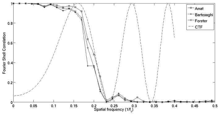
Fig. 7 shows FSC curves of the averages obtained using different dissimilarity scores. Before computing the FSC we aligned both averages with respect to each other to guarantee the best match. TCCC metric performs better than other dissimilarity score in this particular dataset. Just as a guidance, a 0.5 FSC threshold, gives 32Å resolution for TCCC, 38Å for Forster and 37Å for Bartesaghi. Moreover, given the estimated SNR of the dataset and the number of averaged subtomograms, the FSC curves in Fig. 7 and in the simulations shown in Fig. 6 are similar, which allows us to estate that we are mainly limited by the CTF and not by misalignment errors.

Figure 7.

FSC curve for tetramer S-layer (continuous line). Theoretical CTF for imaging conditions (dashed line) assuming 0.1 amplitude contrast and Cs = 3.2mm. Formulas for theoretical CTF from (Frank (2006)-Ch. 3).

4.2.3. Caulobacter Crescentus S-layer of whole cells

Datasets of whole cells of Caulobacter Crescentus were imaged as specified in materials and methods section. The thickness of the sample (approx. 600nm) causes very low SNR. As in the tetramer S-layer, we estimated the SNR by selecting the 1000 boxes with the lowest dissimilarity score to the average. The estimated SNR is 0.072, which situates these datasets in the regime (see Fig. 5) where using TCCC is advantageous. Fig. 8 shows few examples of the raw data.

Figure 8.

XY, XZ, YZ projections of two aligned boxes from raw data for Caulobacter crescentus S-layer. Bar represents 20nm. (A) Same subtomogram as in (B) but with a low-pass filter to visualize main features. The hexagonal pattern is preserved (XY) but the outermembrane feature is almost blurred out. (B) Shows box were missing wedge blurring affects perpendicular to the cell wall. Noise masks all the features. (C) Same subtomogram as in (D) but with a low-pass filter to visualize main features. Outer membrane is visible but hexagonal pattern is almost blurred out. (D) Shows box were missing wedge blurring affects tangential to the cell wall. Again noise masks all the features.

16000 boxes of size 76nm × 76nm × 76nm were extracted from four different datasets. The mask in this case was a cylinder perpendicular to the outer membrane. The S-layer was automatically extracted from each tomogram following the procedure explained in (Gould et al. (2009)). We obtained an initial low resolution template by averaging 200 boxes selected manually by visual inspection from the extracted surface in one dataset. The selection criteria were the overall appearance and location around the cell to uniformly cover missing wedge orientations. Then we crosscorrelated the template along the extracted surface using the TCCC metric. We selected points where the dissimilarity score had a local minima.

As in the previous subsection, we ran the iterative alignment algorithm describe in (Forster et al. (2005)) in two phases. Before splitting the boxes into two datasets, we ran a first cycle of alignment with a heavy band pass filter to obtain a rough orientation of all the particles. Only spatial frequencies between 12nm and 30nm were used for the alignment. After convergence, we selected the boxes where the outer membrane was visible as an anchor point and the TCC value⁶ was above 0.25. The total number of boxes left for alignment was 2089. In this case we used 10000 FFT coefficients for the TCCC dissimilarity score.

To avoid introducing artificial correlations in the averaging, we split the subtomograms in two groups from different tomograms. The first group contains 1106 boxes from tomograms 1 and 2 and the second one contains 983 boxes from tomograms 3 and 4. For each subset of boxes we generated an initial template by averaging 200 randomly selected particles and we ran a separate second cycle of alignment without any band pass filter. The alignment procedure explained above was repeated step by step for each possible metric in order to compare results.

A multi-Z slice image of the resulting averaging can be seen in Fig. 9. The average shows a similar structure to the one obtained from in vitro reconstructions (Smit et al. (1992)). However, we can clearly see a formation of two layers of S-layer (one on top of the other). The periodicity between hexomer centers is 228.09Å and the thickness of one layer of S-layer is 99Å. However, we were not able to resolve the handedness shown in reference (Smit et al. (1992)).

Figure 9.

(A) XZ plane of the C.c. average. Double layer of S-layer is very clear on top of the outer membrane. (B) YZ plane of the C.c. average. (C) Sequential view of slices in the direction perpendicular to the cell wall. Separation between slices is 12Å. Top slice is in the right top corner. Bars represent 30nm.

Some of the boxes contained a single layer of S-layer instead of the two shown in Fig. 9. The TCCC dissimilarity measure is too global to distinguish such a relatively subtle feature compare to the high density outer membrane in a low SNR environment. For this reason, we used projections in X and Y to obtain averaged 1D profiles perpendicular to the outer membrane for each box. In those profiles it was possible to see a “single dip” versus a double “double dip” to differentiate between single and double S-layer.

As in the previous subsection, we calculated FSC curves to estimate resolution of the averaged structure (Fig. 10). In particular, and just as a reference, a 0.5 FSC threshold gives 60Å resolution for TCCC, 63Å for Forster and 66Å for Bartesaghi. Notice that the FSC curves for different dissimilarity scores are much closer in this case than in the tetramer, since we have a better SNR scenario.

Figure 10.

FSC curve for Caulobacter crescentus surface layer (continuous line). Theoretical CTF for the imaging conditions assuming amplitude contrast of 0.2 (dashed line) and Cs = 3.2mm. Formulas for theoretical CTF from (Frank (2006)-Ch. 3).

5. Conclusion

This paper has presented a modification on existing dissimilarity measures to make subtomogram alignment more robust against noise and missing wedge effects. The main idea is that the Fourier transform allows for a sparse representation of subtomograms. In other words, most of the energy is concentrated in a small percentage of the total amount of Fourier coefficients. Thus, in low SNR environments, only a small number of those coefficients are useful for comparing subtomograms. We also show a method on how to estimate the optimal number of coefficients needed based on the data itself.

Making subtomogram alignment more robust to noise allows us to use averaging techniques in thicker specimens or in images with lower defocus, which pushes the first zero CTF limitation. We also showed that if the estimated SNR of our subtomograms is higher than 0.1, it is not worth it to use TCCC, since the technique presented in (Bartesaghi et al. (2008)) using Spherical Harmonics can be faster to find the right orientation and equally precise.

One future improvement point for the TCCC and other cross-correlation based dissimilarity scores is that they fail to capture subtle details that can be masked by high noise and missing wedge effects in the presence of strong features. We have presented a case in the results section where projections in X and Y were needed for each subtomogram to distinguish if they had a single or a double S-layer. Further research in more local dissimilarity measures is necessary.

Finally, we have made the source code available for the community at http://www-vlsi.stanford.edu/TEM/software.htm.

References

- Amat F, Moussavi F, Comolli LR, Elidan G, Downing KH, Horowitz M. Markov random field based automatic image alignment for electron tomography. Journal of Structural biology. 2008 Jul;161 (3):260–275. doi: 10.1016/j.jsb.2007.07.007. [DOI] [PubMed] [Google Scholar]
- Bartesaghi A, Sprechmann P, Liu J, Randall G, Sapiro G, Subramaniam S. Classification and 3d averaging with missing wedge correction in biological electron tomography. Journal of Structural Biolology. 2008;162:436–450. doi: 10.1016/j.jsb.2008.02.008. [DOI] [PMC free article] [PubMed] [Google Scholar]
- Bartesaghi A, Subramaniam S. Membrane protein structure determination using cryo-electron tomography and 3d image averaging. Journal of Structural Biolology. 2009;19:1–6. doi: 10.1016/j.sbi.2009.06.005. [DOI] [PMC free article] [PubMed] [Google Scholar]
- Briggs JAG, Riches JD, Glass B, Bartonova V, Zanetti G, Krusslich HG. Structure and assembly of immature HIV. Proceedings of the National Academy of Sciences. 2009;106 (27):11090–11095. doi: 10.1073/pnas.0903535106. [DOI] [PMC free article] [PubMed] [Google Scholar]
- Clatz O, Delingette H, Talos I, Golby A, Kikinis R, Jolesz F, Ayache N, Warfield S. Robust non-rigid registration to capture brain shift from intra-operative mri. IEEE Trans Med Imaging. 2005 Nov; doi: 10.1109/TMI.2005.856734. [DOI] [PMC free article] [PubMed] [Google Scholar]
- Donoho D. De-noising by soft-thresholding. IEEE Transaction on Information Theory. 1995 May;41:613–627. [Google Scholar]
- Donoho D, Johnstone I, Johnstone IM. Ideal spatial adaptation by wavelet shrinkage. Biometrika. 1993;81:425–455. [Google Scholar]
- Downing KH, Mooney PE. Ccd camera with electron decelerator for intermediate voltage electron microscopy. Microscopy and Microanalysis. 2004;10:1378–1379. doi: 10.1063/1.2902853. [DOI] [PMC free article] [PubMed] [Google Scholar]
- Duchi J, Gould S, Koller D. Projected subgradient methods for learning sparse gaussians. In: McAllester DA, Myllymki P, editors. UAI. AUAI Press; 2008. pp. 145–152. [Google Scholar]
- Fleet PV. Discrete Wavelet Transformations: An Elementary Approach with Applications. Wiley-Interscience; Jan, 2008. [Google Scholar]
- Fodor I, Kamath C. Denoising through wavelet shrinkage: an empirical study. 2003;12:151–160. [Google Scholar]
- Forster F, Medalia O, Zauberman N, Baumeister W, Fass D. Retrovirus envelope protein complex structure in situ studied by cryo-electron tomography. Proceedings of the National Academy of Sciences of the United States of America. 2005;102 (13):4729–4734. doi: 10.1073/pnas.0409178102. [DOI] [PMC free article] [PubMed] [Google Scholar]
- Forster F, Pruggnaller S, Seybert A, Frangakis A. Classification of cryo-electron subtomograms using constrained correlation. Journal of Structural Biolology. 2008;161:276–286. doi: 10.1016/j.jsb.2007.07.006. [DOI] [PubMed] [Google Scholar]
- Frank J. Three Dimensional Electron Microscopy of Macromolecular Assemblies. Academic Press Inc; 1996. [Google Scholar]
- Frank J. Electron Tomography: Methods for Three-dimensional Visualization of Structures in the Cell. 2. Springer; 2006. [Google Scholar]
- Friedman J, Hastie T, Tibshirani R. Sparse inverse covariance estimation with the graphical lasso. Biostat. 2007 Dec; doi: 10.1093/biostatistics/kxm045. kxm045+ [DOI] [PMC free article] [PubMed] [Google Scholar]
- Frigo M, Johnson SG. The design and implementation of FFTW3. Proceedings of the IEEE. 2005;93 (2):216–231. special issue on “Program Generation, Optimization, and Platform Adaptation”. [Google Scholar]
- Gould S, Amat F, Koller D. Alphabet SOUP: A framework for approximate energy minimization. CVPR; 2009. [Google Scholar]
- Grimm R, Singh H, Rachel R, Typke D, Zillig W, Baumeister W. Electron tomography of ice-embedded prokaryotic cells. Byophysics journal. 1998 Feb;74 (2):1031–1042. doi: 10.1016/S0006-3495(98)74028-7. [DOI] [PMC free article] [PubMed] [Google Scholar]
- Heymann JB, Cardone G, Winkler DC, Steven AC. Computational resources for cryo-electron tomography in bsoft. Journal of Structural Biology. 2008;161 (3):232–242. doi: 10.1016/j.jsb.2007.08.002. [DOI] [PMC free article] [PubMed] [Google Scholar]
- Kremer DM, JR, McIntosh J. Computer visualization of three-dimensional image data using imod. 1996 doi: 10.1006/jsbi.1996.0013. [DOI] [PubMed] [Google Scholar]
- Keller Y, Shkolnisky Y, Averbuch A. Algebraically accurate 3-d rigid registration. IEEE Trans Signal Processing. 2006;54 (11):4323–4331. [Google Scholar]
- Liu J, Bartesaghi A, Borgnia M, Sapiro G, Subramaniam S. Molecular architecture of native hiv-1 gp120 trimers. Nature. 2008;455 (7209):109–113. doi: 10.1038/nature07159. [DOI] [PMC free article] [PubMed] [Google Scholar]
- Lui V, Frster F, Baumeister W. Structural studies by electron tomography: From cells to molecules. Annual Review of Biochemistry. 2005;74 (1):833–865. doi: 10.1146/annurev.biochem.73.011303.074112. [DOI] [PubMed] [Google Scholar]
- Malioutov DM, Johnson JK, Willsky AS. Low-rank variance estimation in large-scale gmrf models. ICASSP; 2006. [Google Scholar]
- Mallat S. A Wavelet Tour of Signal Processing. 2. Academic Press; Sep, 1999. (Wavelet Analysis & Its Applications) [Google Scholar]
- Mastronarde D. Dual-axis tomography: an approach with alignment methods that preserve resolution. 1997 doi: 10.1006/jsbi.1997.3919. [DOI] [PubMed] [Google Scholar]
- McIntosh R, Nicastro D, Mastronarde D. New views of cells in 3d: an introduction to electron tomography. Trends in Cell Biology. 2005;15 (1):43–51. doi: 10.1016/j.tcb.2004.11.009. [DOI] [PubMed] [Google Scholar]
- Nicastro D, Schwartz C, Pierson J, Gaudette R, Porter ME, McIntosh JR. The Molecular Architecture of Axonemes Revealed by Cryoelectron Tomography. Science. 2006;313 (5789):944–948. doi: 10.1126/science.1128618. [DOI] [PubMed] [Google Scholar]
- Schmid MF, Paredes AM, Khant HA, Soyer F, Aldrich HC, Chiu W, Shively JM. Structure of halothiobacillus neapolitanus carboxysomes by cryo-electron tomography. Journal of Molecular Biology. 2006;364 (3):526–535. doi: 10.1016/j.jmb.2006.09.024. [DOI] [PMC free article] [PubMed] [Google Scholar]
- Smit J, Engelhardt H, Volker S, Smith SH, Baumeister W. The s-layer of caulobacter crescentus: three-dimensional image reconstruction and structure analysis by electron microscopy. Journal of Bacteriology. 1992;174 (20):6527–6538. doi: 10.1128/jb.174.20.6527-6538.1992. [DOI] [PMC free article] [PubMed] [Google Scholar]
- Sorzano C, Ortiz E, Lpez M, Rodrigo J. Improved bayesian image denoising based on wavelets with applications to electron microscopy. Pattern Recognition. 2006;39 (6):1205–1213. [Google Scholar]
- Tagari M, Newman R, Chagoyen M, Carazo JM, Henrick K. New electron microscopy database and deposition system. Trends in Biochemical Sciences. 2002;27 (11):589–589. doi: 10.1016/s0968-0004(02)02176-x. [DOI] [PubMed] [Google Scholar]
- van Heelm M, Schatz M. Fourier shell correlation threshold criteria. Journal of Structural Biology. 2005;151 (3):250–262. doi: 10.1016/j.jsb.2005.05.009. [DOI] [PubMed] [Google Scholar]
- Wells WM, III, Viola P, Kikinis R. Multi-modal volume registration by maximization of mutual information. Medical Image Analysis. 1996:35–51. doi: 10.1016/s1361-8415(01)80004-9. [DOI] [PubMed] [Google Scholar]
- Winkler H. 3d reconstruction and processing of volumetric data in cryo-electron tomography. Journal of Structural Biolology. 2007;157:126–137. doi: 10.1016/j.jsb.2006.07.014. [DOI] [PubMed] [Google Scholar]
- Wu S, Liu J, Reedy MC, Winkler H, Reedy MK, Taylor KA. Methods for identifying and averaging variable molecular conformations in tomograms of actively contracting insect flight muscle. Journal of Structural Biology. 2009;168 (3):485–502. doi: 10.1016/j.jsb.2009.08.007. [DOI] [PMC free article] [PubMed] [Google Scholar]