Complex System Approaches to Genetic Analysis: Bayesian Approaches

Abstract

Genetic epidemiology is increasingly focused on complex diseases involving multiple genes and environmental factors, often interacting in complex ways. Although standard frequentist methods still have a role in hypothesis generation and testing for discovery of novel main effects and interactions, Bayesian methods are particularly well suited to modeling the relationships in an integrated “systems biology” manner. In this chapter, we provide an overview of the principles of Bayesian analysis and their advantages in this context and describe various approaches to applying them for both model building and discovery in a genome-wide setting. In particular, we highlight the ability of Bayesian methods to construct complex probability models via a hierarchical structure and to account for uncertainty in model specification by averaging over large spaces of alternative models.

I. INTRODUCTION

Bayesian approaches have gained a tremendous amount of popularity in a diverse set of applications including but not limited to: economics, environmental science, bioinformatics, epidemiology, genetics, computer science, political science, and public policy. Within these fields, the Bayesian framework can be applied to a wide range of statistical model classes such as linear regression, generalized linear models, survival analysis, tree models, graphical models, and spatial analyses. The growth in popularity of Bayesian approaches is due in most part to the intuitive nature of inference within the framework, the extreme flexibility of the models, and the computational developments helping to facilitate practical analyses. While this chapter focuses more specifically on the use of Bayesian approaches for complex genetics applications, we begin with a general introduction to the fundamentals of any Bayesian analysis.

A. Fundamentals of a Bayesian approach

The fundamentals of a Bayesian approach lie in Bayes Rule, which is the tool that allows us to revise our current set of beliefs about unknown parameters given a set of observed data Y via conditional probabilities:

$$p(\theta \mid Y)=\frac{p(\theta ,Y)}{p(Y)}=\frac{p(Y\mid \theta )p(\theta )}{\int p(Y\mid \theta )p(\theta )\mathrm{d}\theta }$$

where the integral in the denominator can be replaced by a summation if the probability distribution of θ is discrete. Thus, any Bayesian approach has two major components: (1) defining the joint probability model p(θ, Y) and (2) computing conditional probabilities p(θ ∣ Y). In defining the joint probability model, we must specify the likelihood of the observed data given the parameters of interest, p(Y ∣ θ). This specification is common to both a frequentist approach and a Bayesian approach. However, instead of assuming that the parameters of the model are fixed and their true value is unknown, the Bayesian framework assumes that the parameters themselves are random variables. Thus, to define the joint probability model, we must also specify the prior distribution of the parameters, p(θ), in addition to the likelihood of the observed data.

The above framework assumes that we are interested in making inference on all of the parameters in the probability model. However, in many applications this is not the case. If there is some subset of parameters, θ_I, that we are interested in and the remaining, θ_N, are nuisance parameters we can rewrite the conditional probability for the parameters of interest as:

$$p({\theta }_{\mathrm{I}}\mid Y)=\frac{p(Y\mid {\theta }_{\mathrm{I}})p({\theta }_{\mathrm{I}})}{p(Y)},$$

where p(Y ∣ θ_I) is the marginal likelihood of the data given the parameters of interest for making inference and can be calculated by integrating out the nuisance parameters (or summation for discrete measures):

$$\int p(Y\mid {\theta }_{\mathrm{I}},{\theta }_{\mathrm{N}})p({\theta }_{\mathrm{N}})\mathrm{d}{\theta }_{\mathrm{N}}.$$

Thus, computing conditional probabilities in the Bayesian framework often requires computing high-dimensional integrals (or summations) for both the marginal likelihoods for the parameters of interest, p(Y ∣ θ_I), and the normalizing constant, p(Y).

Finally, in many analyses, there may exist several alternative specifications for the joint model. In a Bayesian analysis, we can incorporate the uncertainty of the specification of the joint model by indexing a specific model by an indicator vector γ. Since we are now considering multiple models, M_γ ∈ M, we can rewrite the joint probability statement as:

$$p(Y,{\theta }_{\gamma },M_{\gamma })=p(Y\mid {\theta }_{\gamma },M_{\gamma })p({\theta }_{\gamma }\mid M_{\gamma })p(M_{\gamma })$$

where θ_γ are the parameters specific to model M_γ. We can therefore make inference on the models themselves by calculating the conditional probabilities:

$$p(M_{\gamma }\mid Y)=\frac{p(Y\mid M_{\gamma })p(M_{\gamma })}{{\mathrm{\sum }}_{M_{\gamma }\in M}p(Y\mid M_{\gamma })p(M_{\gamma })}$$

where p(Y ∣ M_γ) = ∫p(Y ∣ θ_γ,M_γ)p(θ_γ)dθ_γ is the marginal likelihood of the observed data given any of the models of interest.

B. Bayesian advantages

Bayesian approaches come with many advantages. First and foremost, by specifying a probability distribution on the parameters we directly quantify the uncertainty in those parameters given the observed data and achieve statistical conclusions with common sense interpretations. These probability statements allow for a conceptually straightforward approach to inference, in that our prior beliefs specified in p(θ) are updated based on the observed data, Y, via conditional probabilities p(θ ∣ Y). This is quite different from a frequentist approach. A simple example is the Bayesian credible interval versus the frequentist confidence interval. A frequentist 95% confidence interval must be interpreted based on hypothetical repeated sampling in which S repeated samples are taken from the population and, subsequently, S × 0.95 of the estimated parameters would fall within the confidence interval. In contrast, the Bayesian 95% credible interval is interpreted potentially more intuitively as a 95% probability that the true value of the parameter lies within the calculated credible interval.

Another advantage of the Bayesian framework is that it provides a very natural setting for incorporating complex structures, multiple parameters, and procedures for dealing with nuisance parameters (parameters that we do not wish to make inference about). The only restriction within a Bayesian approach is that one must be able to specify a joint probability model for the observed data and parameters of interest. We can therefore include as many parameters to our models as needed and simply marginalize across (i.e., integrate out or sum over) the ones that we are not interested in making inference on. We are also able to incorporate external information in the analysis in an explicit manner by specifying prior probability distributions for the parameters of interest. This is particularly useful in the biological setting where there is often a great deal of external information and incorporating this information can potentially help the practitioner narrow the focus of an otherwise overly complex model. Finally, the Bayesian framework provides a natural setting for incorporating model uncertainty into any analysis by extending the hierarchy and viewing the model itself as a random variable with its own prior distribution.

C. Limitations

Many of the main advantages of a Bayesian approach lie in the specification of prior distributions on the model parameters and in some cases on the models themselves. However, this can also be one of the main limitations of the Bayesian framework. The prior distributions can be specified in either a subjective or objective manner depending about the amount of prior knowledge or external information one has for the parameters or the acceptable degree to which the posterior results are sensitive to the prior specification. However, even if there is a large amount of prior information regarding the parameters of interest or the models themselves, it is not always straightforward to quantify a practitioner’s prior knowledge and elicit prior distributions. Also, if a limited amount of external knowledge exists about the parameters, the question remains about how to specify the priors in an objective (“non-informative”) manner (Thomas et al., 2007a). Advances have been made in both the elicitation of prior distributions and in developing and investigating the asymptotic characteristics of objective priors on both the parameters of interest and the models themselves (discussed in more detail in Sections III and IV).

Another limitation to the Bayesian framework is the complexity of computing conditional probabilities. This complexity lies in the difficulty in performing potentially high-dimensional integrals (or summations) in both the normalizing constant p(Y) and in the marginal likelihood of the data p(Y ∣ θ_I) or p(Y ∣ M_γ). Because of the computational constraints on Bayesian approaches, practitioners were historically limited to choosing only conjugate likelihoods and priors for which conditional probabilities could be calculated in closed form. However, with recent advances in estimating high-dimensional integrals with stable numerical approximations or by simulation via Markov Chain Monte Carlo (MCMC), Metropolis–Hastings (MH), and stochastic model search algorithms, one is much less limited when choosing a joint probability model. These technical advances, as well as software to more easily implement Bayesian models (such as WinBUGS (Speigelhalter et al., 2003) and JAGS (http://sourceforge.net/projects/mcmc-jags)), have lead to an increased popularity of Bayesian approaches (discussed in more detail in Sections III and IV).

D. General model specification

The remainder of the chapter utilizes a generalized linear model framework in which most any type of outcome variable may be analyzed with an appropriate link function. However, for simplicity, we will focus on a binary outcome variable. Let Y be a vector of length n comprised of some binary outcome variable for individual i with expected value

$$E(Y)=\mu$$

with mean vector μ = (μ₁, ⋯, μ_n)^T. Also, for each individual, we assume that p covariates are measured, x₁, ⋯, x_P. We then use generalized regression models to relate the binary outcome variable to a subset of predictor variables. We denote the collection of all possible models by M. An individual model, denoted by M_γ, is specified by an indicator vector γ. Then under each model M_γ, μ is of the general form:

$$M_{\gamma }:\mu =g^{-1}[f(X_{\gamma }){\beta }_{\gamma }]$$

where g is the link function (usually logit whenever Y is binary), f(X_γ) is some general structure or parameterization of a set of covariates, and β_γ are the effects of f(X_γ) on the outcome of interest Y (are parameters of interest θ_γ). A very general structure for the models can be seen as a directed graph in Fig. 3.1. Specifically in this example, the γ indicator allows both the covariates x₁ and x₃ to inform the model and design matrix X_γ, whereas all other covariates (e.g., x₂ and x_p) are excluded. Then f(X_γ) defines the structure or parameterization of these variables in the regression. Finally, the link function, g^{− 1} (·), as well as the regression coefficients, β_γ, relate the structure built in f(X_γ) to disease.

Figure 3.1.

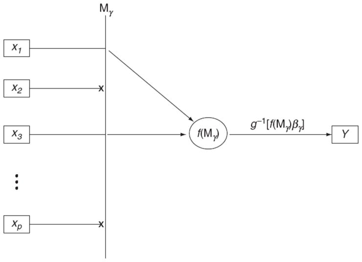
Directed graph summarizing general model structure.

For a simple illustration of the general model structure, we consider a simple logistic regression analysis where the link function is defined as:

$$\mu =\frac{\exp \{f(X_{\gamma }){\beta }_{\gamma }\}}{1+\exp \{f(X_{\gamma }){\beta }_{\gamma }\}}$$

Each model is defined by the indicator γ denoting which of the p possible covariates will be included in the marginal model. In particular, we can have γ be an indicator vector with γ_j = 1 if covariate j is the one included in the marginal model and γ_j = 0 for every i ≠ j. Then the model space M is made up of p single variable models M_γ. Under each model M_γ ∈M the mean vector has the form:

$$M_{\gamma }:\ln \left(\frac{\mu }{1-\mu }\right)={\beta }_0+X_{\gamma }{\beta }_{\gamma }$$

where X_γ is of dimension n × 1 and β_γ is the logarithm of the odds ratio for the single covariate in model M_γ. In the simple marginal case, it is plausible to perform an enumeration of the entire model space M, so typically no stochastic model search algorithm is needed.

Given the general structure that we have developed above, the models that we describe herein can be much more complex than this simple marginal example. In Section II, we review strategies for defining the structure or parameterization of the covariates that is specified in f(X_γ). These strategies can range from the simple marginal analyses to the more complex networks and mechanistic models. In Section III, we tackle the problem of (1) what priors should be placed on the parameters of interest, β_γ, and (2) how to compute the conditional probabilities and estimate β_γ. In Section IV, we incorporate an additional layer into the hierarchy by investigating multiple models M_γ ∈ M. Section IV mainly focuses on (1) defining prior distributions on the model space p(M_γ), (2) how to approximate high-dimensional integrals for marginal likelihoods for the models of interest, p(Y ∣ M_γ), and (3) approximating high-dimensional sums for normalizing constants. Finally, in Section V, we describe methods for determining noteworthiness of the structures defined in Section II and marginally of the covariates themselves.

II. STRUCTURE OF COVARIATES

We begin with the simplest case of a single polymorphism in a single gene, with no genetic or environmental modifiers. In this case, X is comprised of genotypes at a single polymorphism for n individuals and the only consideration in specifying the covariate function f(X) concerns issues of dominance. If the locus is diallelic, with alleles denoted a and A, then we might wish to consider any of the following codings for the genotype X_i:

$$\begin{array}{ll}f(X_i)=1\mathrm{if}X=\mathit{AA}\mathrm{or}\mathit{Aa},0\mathrm{if}X=\mathit{aa}\hfill & \mathrm{Dominant}\hfill \\ f(X_i)=2\mathrm{if}X=\mathit{AA},1\mathrm{if}X=\mathit{Aa},0\mathrm{if}X=\mathit{aa}\hfill & \mathrm{Additive}\hfill \\ f(X_i)=1\mathrm{if}X=\mathit{AA},0\mathrm{if}X=\mathit{Aa}\mathrm{or}\mathit{aa}\hfill & \mathrm{Recessive}\hfill \\ f(X_i)=1\mathrm{if}X=\mathit{AA},\theta \mathrm{if}X=\mathit{Aa},0\mathrm{if}X=\mathit{aa}\hfill & \mathrm{Codominant}\hfill \end{array}$$

(Note that the codominant model entails an additional parameter θ that would be estimated along with the other regression coefficients in β. This is most easily accomplished by fitting a 2-degree of freedom model with two dummy variables for each genotype). In some instances, the choice of coding might be determined by prior biological knowledge, but in the absence of relevant knowledge one would consider each of these possibilities within the general model selection or model uncertainty framework developed in greater detail in Section III.

Most genes have numerous polymorphisms and any candidate pathway study might consider a broad range of genes, so multivariate models are called for. An obvious choice for a binary disease trait might be a logistic regression model

$$\mathrm{logit}(p(Y=1\mid X))={\beta }_0+\sum {\beta }_j{f}_j(X_j)$$

Here, we could incorporate different genetic codings for each variable and therefore we allow the function f_j(X_j) to differ across the covariates. It might also be helpful to consider a hierarchical structure for multiple polymorphisms within genes within pathways. Letting j = 1,…, J index the pathways, and k = 1,…, K_j index the genes within pathway j, and l = 1,…, L_jk polymorphisms within genes, one might extend the logistic model as

$$\mathrm{logit}(p(Y=1\mid X))={\beta }_0+\sum _j{\beta }_j\sum _k{\beta }_{jk}\sum _l{\beta }_{j{k}_l}{f}_{j{k}_l}\left(X_{j{k}_l}\right)$$

with higher level models for the βs constructed in a manner to ensure identifiability. Again, working within the general modeling framework discussed below, one might wish to consider different strategies for selection, shrinkage, or averaging at the polymorphism, gene, or pathway levels.

Gene–environment (G × E) and gene–gene (G × G) interactions introduce a further level of complexity, but the same general framework can be applied. Consider, for example, a model for the joint effect of two polymorphisms X₁ and X₂. The logistic model could then be written as

$$\mathrm{logit}(p(y=1\mid X))={\beta }_0+{\beta }_1{f}_1(X_1)+{\beta }_2{f}_2(X_2)+{\beta }_{12}{f}_{12}(X_{12})$$

where f₁(X₁) and f₂(X₂) denote any of the genetic codings discussed above and f₁₂(X₁₂) could be a simple product X₁X₂ or a term constructed to capture phase information for two polymorphisms in linkage disequilibrium (Conti and Gauderman, 2004), or it could be some more complex epistasis model, such as 1 for X₁₂=(aaBB, aAbB, AAbb), 0 otherwise. See Li and Reich (2000), Moore (2003), Moore et al. (2007), Zhang and Liu (2007), Cordell (2009), Moore and Williams (2009), and Tang et al. (2009) for further discussion of various possibilities for modeling epistasis. Similar codings for G × E interactions are possible (Thomas, 2010a,b). For multiple polymorphisms within the same gene, one might use a haplotype-based model, logit(p(Y= 1 ∣ X)) = β₀ + β₁h₁ (X) + β₂h₂(X), where h₁ and h₂ represent the two haplotypes carried by an individual comprising the set of alleles at the different loci carried on the same chromosome. In the absence of phase information, this would require forming a likelihood by summing over all possible arrangements of the alleles into haplotypes, weighted by their probabilities based on population linkage disequilibrium patterns (Stram et al., 2003).

If specific prior knowledge of the relevant biological process is known, mechanistic approaches may be used to construct more complex models. These models will generally be quite specific to a particular pathway and their mathematical form will depend upon the nature of the pathway. Metabolic pathways, for example, might be modeled in terms of a series of latent variables L(X; m) representing concentrations of intermediate metabolite m. These concentrations could be given by a system of differential equations based on the known pharmacokinetics with rates that depend in some manner on the genotypes encoding the relevant enzymes and their environmental substrates or cofactors (Thomas et al., 2010). The solution to this system then provides a mathematical expression for the covariate function f(X, θ) where X now represents all the genetic and environmental inputs to the system and θ a vector of additional parameters to be estimated for a particular model. For example, Cortessis and Thomas (2003) described a metabolic model for the metabolism of polycyclic aromatic hydrocarbons and heterocyclic amines derived from tobacco smoke and well done red meat as risk factors for colorectal polyps. Each pathway involves several intermediate steps, metabolized by several genes. Using linear kinetics, the metabolic rate parameters were assumed to be lognormally distributed around population means specific to the relevant genotypes. The expected concentration of the final metabolites from each pathway was computed specific to each person’s exposure and genotype, and used as covariates in a logistic model for disease. The model was fitted using MCMC methods, sampling individual metabolic rates and model parameters (regression coefficients, genotype-specific mean rates, and variances) in turn. Further elaboration of this model and comparisons with a BMA analysis using hierarchical models are provided in Conti et al. (2003). As before, one might wish to consider a range of alternative models, such as submodels of a general model including only some subset of the inputs or different codings of dominance or even different mathematical models (e.g., linear vs. Michaelis–Menten kinetics). These approaches have been most extensively developed in the context of population pharmacokinetic models (Best et al., 1995; Bois, 2001; Clewell et al., 2002; Davidian and Gallant, 1992; Gelman et al., 1996; Lunn et al., 2009; Racine-Poon and Wakefield, 1998; Wakefield, 1996), although so far, there has been relatively little attention to genetic variation in metabolic parameters.

III. ESTIMATION

So far, in this chapter, we have focused on how to link and combined the observed data into a probability model. However, the ability to measure numerous factors present many difficulties for analysis (Greenland, 1993). Conventional approaches have relied on either fitting a full model with all the factors included in the probability model or fitting a reduced model determined by some eliminating algorithm. Including all the factors in one model can lead to biased and unreliable estimates due to sparse data when the number of parameters approaches the number of individuals in the sample (Greenland, 2000a,b). Reduced models may avoid this complication, but they fail to account for the correlations that exist between all the factors and can lead to underestimated variance (Robins and Greenland, 1986). Additionally, when statistical tests are used for the numerous exposures, issues of multiple comparisons arise (Thomas et al., 1985). However the model γ is determined, there will be corresponding parameters β_γ that describe the effect on the outcome of interest. For this part of the chapter, we focus on how prior specification on these parameters via hierarchical models can be used to construct complex models for analysis. For example, in a genome-wide association study (GWAS), one might have little or no external information about most SNPs, so such analyses are commonly treated as exploratory; indeed, their “agnostic” or “hypothesis free” nature is commonly touted as one of their advantages. Here, treating each polymorphism as independent may be appropriate. A pathway-driven study, on the other hand, may be able to exploit extensive knowledge about the pharmacokinetics or pharmacodynamics of the pathway. Recently, there has been an intriguing convergence of the two philosophies, with external pathway information being exploited to mine GWAS data for gene sets whose components may not separately attain genome-wide levels of significance but combination implicates particular pathways (Wang et al., 2007; Zhong et al., 2010), or by exploring GWAS data to discover hitherto unsuspected sets of genes that may share a common biological function (Sebastiani et al., 2005).

Rather than treating each factor independently, specification of the relations among the observed data with two or more stages can be used to create an intricate joint probability model. While each stage may be relatively simple and easy to understand, the entire model may be much more sophisticated, with the aim to more accurately model the underlying complex processes. Additionally, by providing a joint probability model for all exposures, hierarchical modeling offers a potential solution to problems of multiple comparisons (Greenland and Robins, 1991; Thomas et al., 1985). As one of the first examples in genetic epidemiology, Thomas et al. (1992) used hierarchical modeling to jointly evaluate numerous human leukocyte antigen (HLA) alleles and their association to insulin-dependent diabetes mellitus (IDDM), while incorporating several environmental risk factors.

The addition of higher stage information can substantially improve the accuracy and stability of effect estimates (Greenland, 2000a,b; Greenland and Poole, 1994; Morris, 1983). However, to achieve this improvement, the model hierarchy must be specified in a manner that efficiently uses the data and is scientifically plausible (Rothman and Greenland, 1998).

While a conventional model fits a single probability level to describe the relation between the multiple factors and the outcome, hierarchical models incorporate higher level prior distributions to explain the relations among the parameters. Although multiple levels of prior structure can be constructed, in practice there is a limit to the number of levels that can be feasibly estimated from the data without relying too much on a strongly specified prior. Consider the general scenario with multiple factors, X, and outcome, Y. The first-probability model at the individual-level can be specified as:

$$Y\mid X,\beta \sim p(Y\mid X,\beta )$$

As before, Y and X are observed data and β are the corresponding coefficients of risk associated with a one-unit increase for each factor. Subsequently, probability models are placed on the parameters, β, assuming that they come from a common probability distribution.

$$\begin{array}{l}\beta \mid \theta \sim p(\beta \mid \theta )\hfill \\ \theta \sim p(\theta )\hfill \end{array}$$

Such a hierarchy can apply dependencies to the estimates of the parameters β through the structure of p(β ∣ θ). These dependencies are often modeled conditionally on certain parameters, θ, called hyperparameters and these hyperparameters can also be assigned probability distributions, p(θ). An important assumption here is that the parameters are exchangeable. That is, the parameters (β₁, …, β_m) are exchangeable in their joint distribution if p(β₁, …, β_m) is invariant to permutations of the indexes (1, …, m) (Gelman, 1995). Consequently, given no other information, other than the data itself, there is no prior ordering or grouping of the parameters (β₁, …, β_m). If this assumption holds, we may assume that the corresponding coefficients for the exposures, β, are drawn from the same common population distribution.

The general hierarchical modeling framework presented in the above equations provides a quite flexible framework to model complex systems. For example, p(β ∣ θ) specified as a normal distribution centered at zero is akin to ridge regression, a frequentist robust regression technique (Sorenson and Gianola, 2002). Similarly, a double exponential for p(β ∣ θ) is equivalent to the Lasso procedure (Park and Casella, 2008; Chen et al., 2010). To demonstrate the flexibility and nuances of specifying such a hierarchy, consider a specific analysis of case-control data with numerous genetic and environmental factors. A specific hierarchical model can be specified as:

$$\begin{array}{c}\mathrm{logit}(p(Y=1\mid X))={\beta }_0+\sum {\beta }_j{f}_j(X_j)\\ \beta \sim \mathit{MVN}(\mathbf{Z}\pi ,\mathit{\sum })\end{array}$$

where X is a design matrix of genetic and environmental factors for the individuals within the study, Z contains second-stage covariates for each of the environmental and genetic factors reflecting higher level, often prespecified relations, π is a column vector of coefficients corresponding to these higher level effects on disease, and Σ is a matrix specifying the residual covariance of the second-stage covariates. There are many possible types of information that could be used for defining Z. In genetics, this could define simple indicator variables for which pathway(s) each gene is thought to be active (Hung et al., 2004), information extracted systematically from genomic or pathway ontologies (Conti et al., 2009; Thomas et al., 2007b), experimental information such as eQTLs from cell cultures (Zhong et al., 2010), in silico predictions based on evolutionary conservation or predicted effect on protein conformation (Rebbeck et al., 2004), or predictions from simulations of the pathway (Thomas et al., 2010). Of course, multiple sources could, in principle, be combined and additional levels can easily be incorporated, such as separate models for SNPs within genes and genes within pathways (Conti and Gauderman, 2004) or for main effects and interactions (Conti et al., 2003).

Overall this hierarchy will result in posterior estimates for the association parameters that are an inverse-variance weighted average between the conventional estimates from the logistic regression only and the estimated conditional second-stage means, Zπ. To see this more clearly, consider a simple weighted regression approach for estimation. Here, the second-stage estimated prior means, Zπ̃, and corresponding estimated covariance matrix, (Z^T WZ) ^{− 1}, can be obtained from a weighted least squares regression, π̃ = (Z^TWZ) ⁻¹ZWβ̂, where W= (V+Σ) ^{− 1}, and V is a diagonal matrix with elements equal to the square of the estimated standard errors for β̂ (Morris, 1983). Averaging the firstand second-stage estimates yields posterior estimates

$$\stackrel{\sim }{\beta }=\mathit{BZ}\stackrel{\sim }{\pi }+(I\mathrm{-}B)\widehat{\beta }.$$

The estimate of the covariance matrix is given by C̃ = V̂(I− (I − H)^T B), where H = Z(Z^TWZ) ^{− 1}Z^TW and B is the estimated shrinkage matrix

$$B=\mathit{WV}={(V+\mathit{\sum })}^{-1}V$$

From these equations, we can see that if the maximum likelihood first-stage estimates, β̂, have large variance, V̂, relative to the prior variance, Σ, then B will also be large. As a result, the hierarchical analysis has several important differences from the conventional, single-stage logistic regression analysis. First, the conventional analysis has no constraints on the first-stage regression coefficients, β. For example, if we model the effects of smoking on lung cancer, we would expect the effect estimate, β̂, to be quite high. But even in this extreme case, we would not expect outrageously high odds ratios. It makes sense to incorporate this expectation into our analysis by including a probability distribution for the effect estimates that weights more probable estimates higher. This may be done by setting the elements in the Z matrix to zero and allowing Σ to reflect our prior beliefs about the extent of the probability distribution of the first-stage coefficients, β. However, if we have information regarding the relations between the factors, we may incorporate that information into the Z design matrix and account for the effects due to these dependencies. In this case, Σ reflects residual covariance or associations between the first-stage parameters, β, after accounting for the relations defined in Z. If we allow the elements of Σ to go to infinity—that is, we have no prior belief regarding the distribution of the residual effects—the final estimates of effect will disregard any second-stage information and be equal to the first-stage conventional maximum likelihood estimates. If we set the elements of Σ to zero, believing that there are no residual effects beyond the relationships defined in Z, then the final estimates will be equal to the estimated second-stage conditional means, Zπ. Thus, Σ acts as a smoothing parameter, controlling the amount of shrinkage from the conventional first-stage maximum likelihood estimates toward the second-stage conditional means. Within this context, the specification of Σ is very flexible. Joint modeling is often represented by setting Σ = τ²D, where τ² > 0 represents the overall variance of the effect estimates and D is a positive definite correlation matrix describing the correlation between the effect estimates for any two pairs of polymorphisms. Conti and Witte (2003) utilized this specification to set D to the expected decay of linkage equilibrium. Closely related to this is a Gaussian conditional autoregression specification where D = (I − ρA) ^{− 1} (Wakefield et al., 2000). Here, the elements within A describe the spatial weights between any two polymorphisms and ρ is interpreted as the strength of the spatial dependence. Thomas et al. (2010) recently investigated the use of this model in the genetics context using prior gene–gene connection information such as from gene coexpression experiments to define A. The normal g-prior defines the covariance matrix as the inverse of the Fisher information matrix multiplied by a constant g, Σ = g(X^TX) ^{− 1} (Zellner, 1986). This ensures that the correlation structure in the prior distribution matches the structure in the likelihood with either g being determined via information criterion (such as AIC) or estimated with a prior specified for g.

The general hierarchical model specified above often leads to analytically intractable computations of posterior distributions p(β ∣ Y) when estimating β. Approximate methods can be used for parameter estimation and can include a semi-Bayes, empirical Bayes, or fully Bayesian approaches. In a semi-Bayes approach, the value for τ² is prespecified as opposed to estimating the value from the data. This may be advantageous if the estimate of τ² is itself highly unstable (Greenland, 1993, 1997; Greenland and Poole, 1994). However, because the most appropriate value for τ² is unknown it is standard to perform a sensitivity analysis to evaluate how dependent the posterior estimates are to the choice of τ². In contrast, an empirical Bayes approach uses the marginal distribution of τ² to obtain a point estimate that is then used to evaluate the joint posterior distribution for the log odds ratios, β (Efron and Morris, 1975; Greenland and Poole, 1994; Morris, 1983; Searle et al., 1992). Semi-Bayes and empirical Bayes methods, such as two-stage weighted least squares, joint iterative weighted least squares and penalized quasi-likelihood (Breslow and Clayton, 1993; Greenland, 1997), suffer from the inability to reflect our uncertainty for τ² in the final posterior estimates for the log of the odds ratio. A fully Bayesian approach using MCMC methods avoids this and incorporates the uncertainty about τ² into the analysis by evaluating the full joint posterior distribution through simulation. However, these methods contain many potential difficulties and care must be taken when implementing and interpreting the final results (Gelman, 1995; Gilks et al., 1996).

Within the hierarchical modeling framework, connections to model selection procedures can be easily made by assuming a mixture model for p(β ∣ θ). George and McCulloch (1993) introduced a Stochastic Search Variable Selection (SSVS) algorithm by introducing a latent variable, W_j = 0 or 1, indicating whether term j is included in the model with a mixture prior for the coefficients:

$$p\left({\beta }_j\mid \tau ,\psi \right)=\{\begin{array}{cc}N\left(0,{\tau }^2\right),& \mathrm{if}{W}_j=0\hfill \\ N\left(0,{(\psi \tau )}^2\right),& \mathrm{if}{W}_j=1\hfill \end{array}$$

Here, ψ is a variance inflation factor defining the separation between two normal distributions centered at zero. Since τ² functions as a smoothing parameter, a specification of τ² = 0 defines a point mass at zero for those terms not included in the model (see “spike and slab” discussion in Section IV).

The benefits of a Bayesian approach to parameter specification need not be limited to the case of numerous factors. Consider a simple scenario in which the aim is to estimate a statistical or multiplicative interaction between two factors, a genetic factor G and a dichotomous environmental factor E. In the conventional single-level case-control analysis, the departure from a multiplicative interaction model can be estimated as β_GE^CC from the following logistic model:

$$\mathrm{logit}(p(Y=1\mid G,E))={\beta }_0^{\mathrm{CC}}+{\beta }_{\mathrm{G}}^{\mathrm{CC}}G+{\beta }_{\mathrm{E}}^{\mathrm{CC}}E+{\beta }_{\mathrm{GE}}^{\mathrm{CC}}\mathrm{GE}$$

Under the assumption of a rare disease and independence of the two factors in the source population, a case-only analysis may be used to estimate an equivalent interaction β_GE^CO, as well:

$$\mathrm{logit}(p(E=1\mid Y=1,G))={\beta }_0^{\mathrm{CO}}+{\beta }_{\mathrm{GE}}^{\mathrm{CO}}G$$

Leveraging these two approaches, Mukherjee and Chatterjee (2008) constructed a hierarchical prior for the case-control estimate as a function of the case-only estimate, ${\beta }_{\mathrm{GE}}^{\mathrm{CC}}\sim N\left({\beta }_{\mathrm{GE}}^{\mathrm{CO}},{\tau }^2\right)$. The result is a shrinkage estimator similar to that outlined above but one that is a weighted average between the case-only and case-control estimates:

$${\stackrel{\sim }{\beta }}_{\mathrm{GE}}=B{\beta }_{\mathrm{GE}}^{\mathrm{CO}}+(1\mathrm{-}B){\beta }_{\mathrm{GE}}^{\mathrm{CC}}$$

The weight B is defined as:

$$B=\frac{{\widehat{V}}_{\mathrm{CC}}}{{\widehat{V}}_{\mathrm{CC}}+{\theta }_{\mathrm{GE}}^2}.$$

The amount of shrinkage is controlled by θ_GE², the maximum likelihood estimate of the log of the G–E odds in controls relative to the estimated variance (V̂_CC) of the case-control estimator β_GE^CC. Thus, the final estimate β̃_GE shares the efficiency of the case-only estimate when the two factors are estimated to be independent within the controls and the robustness of the case-control estimate otherwise.

Further demonstrating the close connection between hierarchical mixture models and Bayesian model averaging, Li and Conti (2009) proposed a similar weighted average. However, in their Bayesian model averaging approach, the weight is defined as B = p(M_CO ∣ Y), the posterior probability of the case-only model relative to the case-control model. This is calculated as:

$$p(M_{\mathrm{CO}}\mid Y)=\frac{p\left(Y\mid M_{\mathrm{CO}}\right)p\left(M_{\mathrm{CO}}\right)}{p\left(Y\mid M_{\mathrm{CO}}\right)p\left(M_{\mathrm{CO}}\right)+p\left(Y\mid M_{\mathrm{CC}}\right)p\left(M_{\mathrm{CC}}\right)},$$

where p(M_γ) is the prespecified or semi-Bayes prior probability for model γ (either the case-only or case-control models) and p(Y ∣ M_γ) is the integration of the likelihood of model M_γ, estimated through a Laplace transformation. For a comparable likelihood between the two models they frame both models in a log-linear framework. Similar to the approach of Mukherjee and Chatterjee (2008), since the likelihood of the case-control model is a function of the estimated G–E association in the controls, θ_GE plays an important role in determining the weight.

IV. MODEL UNCERTAINTY

Model selection is the process of combining data and prior information to select among a group of statistical models M_γ ∈M. In building a model, decisions to include or exclude covariates as well as uncertainty in how to code the covariates in the design matrix X_γ for any given model M_γ are based both on the prior hypotheses and the data. With many potential covariates, these decisions become difficult. Some algorithms will select variables to be included in the model, but only return a single “best” model (e.g., stepwise regression). These methods fail to account for model uncertainty, that is, a number of models may fit the data equally well. In a Bayesian framework, model uncertainty can be addressed by basing inference on the posterior distribution of models.

One simple example of the model uncertainty framework is in variable selection, where each model is defined by a distinct subset of p covariates and is specified by the indicator vector γ which is comprised of a set of p 0s or 1s indicating the inclusion or exclusion of each of the covariates in model M_γ. Then in the logistic regression framework each model is defined as:

$$\mathrm{logit}\left(p\left(Y=1\mid X,M_{\gamma }\right)\right)={\beta }_0+X_{\gamma }{\beta }_{\gamma }$$

where X_γ is the design matrix that is made up of the p_γ covariates in model M_γ, and β_γ is a p_γ dimensional vector of model-specific regression coefficients. Here, the model space M_γ ∈M is made up of 2^p possible models.

In general, the main quantity of interest that needs to be calculated is the posterior probability for any model M_γ given by the equation:

$$p\left(M_{\gamma }\mid Y\right)=\frac{p\left(Y\mid M_{\gamma }\right)p\left(M_{\gamma }\right)}{\sum p\left(Y\mid M_{\gamma }\right)p\left(M_{\gamma }\right)}$$

where p(Y ∣ M_γ) is the marginal likelihood, p(M_γ) is the prior probability for a particular model, and the denominator is a constant found by summing over the entire model space. When p is small, one can exhaustively visit all the possible models. For p covariates, there are t= 2^p − 1 possible terms (including main effect and interaction terms), and 2^t possible models. As p increases the model space M quickly outgrows what is computationally feasible, and an approximation of the posterior distribution of models by MCMC methods is required. When carefully designed, these approaches can efficiently search through the model space.

Bayesian approaches introduce an additional layer of uncertainty to the model by specifying priors on the model space itself p(M_γ). By Ockham’s razor, the simplest models that explain our observations are preferred. This guidance can be formalized as a prior (Jefferys and Berger, 1991). Many approaches adopt a “spike and slab” prior distribution, where most regression coefficients are zero (the spike) and a few coefficients have some effect (slab) (Mitchell and Beauchamp, 1988). Others incorporate some form of lasso (lease absolute shrinkage and selection operator), which either shrinks coefficients or sets them to zero (Tibshirani, 1996). Some approaches directly penalize model complexity. Chen and Chen (2008) introduced a penalty term to the Bayesian information criterion (BIC) based on the size of the model space with the same number of variables as the current model. Wilson et al. (2010) introduced a Beta-Binomial prior on model size that holds the prior odds of any association constant as p increases, thus limiting false discoveries.

Biological knowledge can also be incorporated into a prior on the model space. This knowledge can be used as a prior on the probability that a coefficient is involved (p(γ_j = 1)) and the effect given that it is involved. As discussed earlier, SSVS achieves this using a mixture prior for variable j, such that:

$${\beta }_j={\gamma }_{j}N\left({\mu }_j,{\tau }_j\right)+\left(1-{\gamma }_j\right)\delta (0)$$

where δ(0) is the spike, and N(μ_j, τ_j) is the prior on the mean and variance of β_j given that it is not zero (Conti et al., 2003, 2009). Biological knowledge can also form the basis for model priors. For example, a hypothesized biological pathway can be used as a reference “prior topology,” and structures closer to this reference have greater prior probability (Baurley et al., in press).

MCMC methods are extremely flexible. Here, we describe the general design of the MH algorithm. A random walk MH algorithm explores models in the neighborhood of the current model (Robert and Casella, 2004). A random change to the current model M_t−1 is performed to create the proposed model M′. The changes allowed are often specific to the model structure. For instance, a change to a logistic regression model could be the addition or removal of a regression term. A new model is accepted as M_t with probability,

$$\alpha =\min \left(1,\frac{p\left(Y\mid M\prime \right)p\left(M\prime \right)q\left(M_{t-1}\mid M\prime \right)}{p\left(Y\mid M_{t-1}\right)p\left(M_{t-1}\right)q\left(M\prime \mid M_{t-1}\right)}\right)$$

where p(Y ∣ M′) is the marginal likelihood of the model, p(M′) is the model prior, and q( ∣ ) is the proposal density. There are many choices for the model prior and proposal density, and these influence the performance and behavior of the algorithm. After convergence, models are sampled from the posterior distribution of models.

For model selection applications where p is large, MCMC algorithms may have difficulties traversing a multimodal posterior distribution and poor efficiency arising from the scale of the model space. Recently, new samplers have been introduced that overcome some of these issues by exploiting multiple chains running in parallel. Evolutionary stochastic search (ESS) utilizes a “population” of MCMC chains operating at different temperatures, with hotter chains moving about the model space quicker than cooler chains. The chains are updated with local and global moves. Local moves explore models in the neighborhood of the current model (i.e., random walk) whereas global moves allow a chain to move to a new area of the model space by swapping states with another chain. This algorithm has been incorporated into the MISA (Multilevel Inference of SNP Associations) framework that computes posterior probabilities and Bayes factors (BFs) at the SNP, gene, and global level (Wilson et al., 2010).

In a different strategy, parallel chains are utilized to tune the MCMC proposal density to better approximate the posterior density. This improves efficiency because less time is spent proposing models with little evidence. The methodology (known as PEAK) organizes the model space into subspaces linked through a graph (Baurley et al., 2009). This graph can be informative, meaning it is derived from an ontology or domain expert or simply symmetric (a divide and conquer approach to the model space). The chains running on smaller model spaces tune the proposal densities for chains operating on larger spaces. The method has been applied to a childhood asthma case-control dataset and discovered several oxidative stress genes and gene–gene interactions for further investigation.

We can also allow for model uncertainty when incorporating interactions of covariates in the structure of the interactions and the covariates being included in the interaction. For instance, in logic regression, the model is of the form,

$$\mathrm{logit}(\mathrm{p}(Y=1\mid X))={\beta }_0+\sum {\beta }_j{f}_j\left(X_j\right)$$

where f_j(X_j) is a Boolean combination of the risk factors (called a logic tree) and β_j is the net effect of that Boolean combination (Ruczinski et al., 2003). The model allows for L logic trees, each containing observed variables and logical operators (AND, OR, and NOT) that can represent different types of interactions. Baurley et al. (2010) extended this framework to continuous variables where the function f_j(X_j) became the net effect of a pathway structure (called a topology) such that,

$$f_j\left(X_j\right)={\theta }_{n,1}{\mathrm{par}}_1\left(X_n\right)+{\theta }_{n,2}{\mathrm{par}}_2\left(X_n\right)+\left(1-{\theta }_{n,1}-{\theta }_{n,2}\right){\mathrm{par}}_1\left(X_n\right){\mathrm{par}}_2\left(X_n\right)$$

where par₁ (X_n) and par₂(X_n) return the values of the parents of X_n in the topology (either an observed variable Z or a latent variable X) and θ_n,1 and θ_n,2 are parameters that can represent a range of interaction types.

V. DETERMINING NOTEWORTHINESS

Given the above defined models, we are interested in addressing two questions: (1) globally, is there an association between any of our covariates of interest and the outcome? and (2) if there is a global association, which individual covariates or structures of covariates are most likely driving the association?. Both of the questions can be answered via multilevel posterior probabilities (or conditional probabilities) and Bayes factors.

A. Global posterior quantities

We are first interested in addressing the following global hypotheses:

• H_A: At least one covariate is associated with the outcome of interest.

• H₀: There is no association between the covariates of interest and the outcome.

The extent to which the data supports each of the hypotheses is calculated via posterior probabilities p(H_A ∣ Y):

$$p(H_A\mid Y)=\frac{p(Y\mid H_A)p(H_A)}{p(Y\mid H_A)p(H_A)+p(Y\mid H_0)p(H_0)},$$

and p(H₀ ∣ Y) = 1 − p(H_A ∣ Y). These quantities are a function of both the marginal likelihood of the hypotheses (p(Y ∣ H_A) and p(Y ∣ H₀)) and the prior distributions placed on the hypotheses (p(H_A) and p(H₀)). In particular, in the Bayesian variable selection framework the posterior probability of the alternative hypothesis that at least one covariate is associated takes on the form:

$$p(H_A\mid Y)=\sum _{M_{\gamma }\ne M_0}p(M_{\gamma }\mid Y),$$

where we simply sum up the posterior probability for all non-null models (M_γ ≠ M₀) . Also, the posterior probability of the null hypothesis takes on the form:

$$p(H_0\mid Y)=p(M_0\mid Y).$$

Decisions based on which hypothesis is more likely can then be made based on the posterior probabilities. These posteriors have an intuitive interpretation of the probability of the hypothesis conditional upon seeing the data.

Given that there is posterior evidence of the global hypothesis that at least one of the covariates of interest is associated with the outcome, we are further interested in answering the question of which covariate is most likely driving the association. This question can be answered based on marginal posterior probabilities. In particular, in the Bayesian variable selection framework, the posterior probability of any covariate X_i being associated can be calculated as:

$$p({\gamma }_i=1)=\sum _{M_{\gamma }\in M:{\gamma }_i=1}p(M_{\gamma }\mid Y),$$

which is simply the sum of the posterior probability for every model that includes the covariate X_i.

One should note that in case of calculating inclusion probabilities for highly correlated covariates (i.e., SNPs in LD) there is an expected dilution in the corresponding posterior probabilities due to the covariates providing competing evidence for an association and therefore the posterior probability of an association will be diluted or distributed across several correlated covariates. We therefore extend this notion of marginal covariate inclusion probabilities to group inclusion probabilities (where we assume less correlation will exist across the groups) and achieve multilevel posterior probabilities (Wilson et al., 2010) by considering the posterior probability that at least one covariate within a given group is associated. One example would be in genetic association studies to group SNPs according to their corresponding gene and calculate gene inclusion probabilities that are simply the sum of the posterior probability of all models that include at least one of the SNPs within the given gene.

In the Bayesian framework, we can also calculate the ratio of the weight of evidence for any two hypotheses (H_A vs. H₀) based on BFs:

$$\mathit{BF}[H_A:H_0]=\raisebox{1ex}{$\frac{p(H_A\mid Y)}{p(H_0\mid Y)}$}\!\left/ \!\raisebox{-1ex}{$\frac{p(H_A)}{p(H_0)}$}\right..$$

A BF (Kass and Raftery, 1995) compares the posterior odds of any two hypotheses to the prior odds and measures the change of evidence provided by data for one hypothesis to the other. Goodman (1999) and Stephens and Balding (2009) provide a discussion of the usefulness of BFs in the medical context and Wakefield (2007) and Whittemore (2007) illustrate their use in controlling false discoveries in genetic epidemiology studies. Jeffreys (1961) presents a descriptive classification of BFs into “grades of evidence” (reproduced in Table 3.1) to assist in their interpretation, which is also reproduced in the work of Kass and Raftery (1995). Thus, decisions about which hypothesis are more likely can be made based on these grades of evidence.

Table 3.1.

Jeffreys Grades of Evidence (Jeffreys, 1961)

Grade	BF(HA:H0)	Evidence against H0
1	1–3.2	Indeterminate
2	3.2–10	Positive
3	10–31.6	Strong
4	31.6–100	Very strong
5	>100	Decisive

Jeffreys (1961) was well aware of the issues that arise with testing several simple alternative hypotheses against a null hypothesis, noting that if one were to test several hypotheses separately, then by chance one might find one of the BFs to be less than one even if all null hypotheses were true. He suggested that, in this context, the BFs needed to be “corrected for selection of hypotheses.” However, it was not clear what Jeffreys meant explicitly by this correction. Experience with genetic studies shown that detectable SNP associations are relatively infrequent. For this reason, Stephens and Balding (2009) suggest that marginal BFs calculated assuming equal prior odds should alternatively be interpreted in light of prior odds more appropriate to the study at hand (leading to a much greater significance threshold than Jeffreys suggests). Another approach to the problem of exploring multiple hypotheses is to embed each of the potential submodels (corresponding to a subset of SNPs) into a single hierarchical model. Unlike the marginal (one-at-a-time) BFs indicated by Stephens and Balding (2009) that are independent of the prior odds on the hypotheses, SNP BFs computed in the Bayesian variable selection framework are based on comparing composite hypotheses and hence do depend on the prior distribution over models. Thus, it is important to select priors on the model space that have an implicit multiplicity correction. One example of this is the Beta-Binomial prior with hyperparameters a= 1 and b= p (the number of SNPs in the study) suggested by Wilson et al. (2010). By diluting the prior marginal inclusion probability, this maintains constant global prior odds of an association even as the number of SNPs in the analysis increases.

VI. CONCLUSIONS

Bayesian approaches to complex analysis are becoming more and more popular. In this chapter, we have attempted to demonstrate that a Bayesian perspective provides a flexible framework for complex genetic analyses by breaking the problem into several components: (1) specification of a model structure via the covariates or combination of covariates; (2) estimation and prior specification of the corresponding parameters; and finally, (3) incorporation of the uncertainty of the specified model structure. The themes presented here focus on a generalization of Bayesian hierarchical models and their flexibility to allow the analyst to easily incorporate complex structures, multiple parameters, deal with nuisance parameters, and have common sense interpretations of the parameters of interest. Unfortunately, this added flexibility over more commonly used frequentist methods comes with the added complexity of computing conditional probabilities (high-dimensional integrals or summations) and eliciting subjection or, when there is a lack of prior knowledge, developing objective prior distributions. However, in this chapter, we discuss advances that have been made in both estimating high-dimensional integrals and in the elicitation of prior distributions.

The most notable advantage of a hierarchical perspective to data analysis is that each stage becomes relatively easy to construct, understand, and interpret. Upon aggregating these stages, the overall model can be quite complex. However, even in the face of these complexities, inference is feasible by leveraging the specified hierarchy. The potential advantages of hierarchical models are often contingent upon the ability of the model, both the individual stages and the overall probability model, to provide an accurate representation of the true data generating mechanism. The potential fear that the prior will overwhelm the data has potentially lead many to shun Bayesian approaches. While all analytic models make some level of assumptions, it is important to understand that the specification of priors is not solely subjective. A prior on parameters simply specifies or structures an exchangeable class of parameters. It does not prespecify the degree to which those parameters may differ. Further uncertainty is incorporated by also searching over alternative models. Sensitivity analysis should be performed to gauge the dependence of final inference upon the prior structure. However, the goal of such sensitivity analysis should be to better understand the balance between the data and the prior. It should not be done to ensure that final inference is reflective of the data only and not the prior. After all, our goal is to leverage the hierarchy and the external information to gain potential advantages with inference. In complex systems analysis of biological processes, we believe that a Bayesian perspective via hierarchical models is appropriate since these processes often follow a conceptual hierarchy, that is, SNPs within genes, genes within biochemical pathways, pathways within physiological processes, physiological processes within social networks. Furthermore, recent advances in technology now make it feasible to generate massive amounts of data aimed at measuring the elements in this hierarchy (i.e., genomics, proteomics, metabolomics). To integrate such data will require complex models that are reflective of the overall process, but simplistic and intuitive at each stage of construction.

References

- Baurley JW, Conti DV, Gauderman WJ, Thomas DC. Discovery of complex pathways from observational data. Stat Med. 2010;29(19):1998–2011. doi: 10.1002/sim.3962. [DOI] [PMC free article] [PubMed] [Google Scholar]
- Best NG, Tan KK, et al. Estimation of population pharmacokinetics using the Gibbs sampler. J Pharmacokinet Biopharm. 1995;23(4):407–435. doi: 10.1007/BF02353641. [DOI] [PubMed] [Google Scholar]
- Bois FY. Applications of population approaches in toxicology. Toxicol Lett. 2001;120(1–3):385–394. doi: 10.1016/s0378-4274(01)00270-3. [DOI] [PubMed] [Google Scholar]
- Breslow NE, Clayton DG. Approximate inference in generalized linear mixed models. J Am Stat Assoc. 1993;88:9–25. [Google Scholar]
- Chen JH, Chen ZH. Extended Bayesian information criteria for model selection with large model spaces. Biometrika. 2008;95(3):759–771. [Google Scholar]
- Chen LS, Hutter CM, Potter JD, Liu Y, Prentice RL, Peters U, Hsu L. Insights into colon cancer etiology via a regularized approach to gene set analysis of GWAS data. Am J Hum Genet. 2010;86(6):860–71. doi: 10.1016/j.ajhg.2010.04.014. [DOI] [PMC free article] [PubMed] [Google Scholar]
- Clewell HJ, Andersen ME, et al. A consistent approach for the application of pharmacokinetic modeling in cancer and noncancer risk assessment. Environ Health Perspect. 2002;110:85–93. doi: 10.1289/ehp.0211085. [DOI] [PMC free article] [PubMed] [Google Scholar]
- Conti D, Gauderman W. SNPs, haplotypes, and model selection in a candidate gene region: The SIMPle analysis of multilocus data. Genet Epidemiol. 2004;27:429–441. doi: 10.1002/gepi.20039. [DOI] [PubMed] [Google Scholar]
- Conti DV, Witte JS. Hierarchical modeling of linkage disequilibrium: Genetic structure and spatial relations. Am J Hum Genet. 2003;72(2):351–363. doi: 10.1086/346117. [DOI] [PMC free article] [PubMed] [Google Scholar]
- Conti DV, Cortessis V, et al. Bayesian modeling of complex metabolic pathways. Hum Hered. 2003;56(1–3):83–93. doi: 10.1159/000073736. [DOI] [PubMed] [Google Scholar]
- Conti DV, Lewinger JP, et al. Using ontologies in hierarchical modeling of genes and exposures in biologic pathways. In: Swan GE, editor. Phenotypes and Endophenotypes: Foundations for Genetic Studies of Nicotine Use and Dependence. Vol. 20. NCI Tobacco Control; Bethesda, MD: 2009. pp. 539–584. [Google Scholar]
- Cordell HJ. Detecting gene–gene interactions that underlie human diseases. Nat Genet. 2009;10:392–404. doi: 10.1038/nrg2579. [DOI] [PMC free article] [PubMed] [Google Scholar]
- Cortessis V, Thomas DC. Toxicokinetic genetics: An approach to gene–environment and gene-gene interactions in complex metabolic pathways. In: Bird P, Boffetta P, Buffler P, Rice J, editors. Mechanistic Considerations in the Molecular Epidemiology of Cancer. IARC Scientific Publications; Lyon, France: 2003. [PubMed] [Google Scholar]
- Davidian M, Gallant AR. Smooth nonparametric maximum likelihood estimation for population pharmacokinetics, with application to quinidine. J Pharmacokinet Biopharm. 1992;20(5):529–556. doi: 10.1007/BF01061470. [DOI] [PubMed] [Google Scholar]
- Efron B, Morris C. Data analysis using Stein’s estimator and its generalizations. J Am Stat Assoc. 1975;70:311–319. [Google Scholar]
- Gelman A. Bayesian Data Analysis. Chapman & Hall; London/New York: 1995. [Google Scholar]
- Gelman A, Bois F, et al. Physiological pharmacokinetic analysis using population modeling and informative prior distributions. J Am Stat Assoc. 1996;91:1400–1412. [Google Scholar]
- George EI, McCulloch RE. Variable selection via Gibbs sampling. JASA. 1993;88:881–889. [Google Scholar]
- Gilks W, Richardson S, editors. Markov Chain Monte Carlo in Practice. Chapman & Hall; London: 1996. [Google Scholar]
- Goodman SN. Toward evidence-based medical statistics. 2: The Bayes factor. Am Soc Intern Med. 1999;130:1005–1013. doi: 10.7326/0003-4819-130-12-199906150-00019. [DOI] [PubMed] [Google Scholar]
- Greenland S. Methods for epidemiologic analyses of multiple exposures: A review and comparative study of maximum-likelihood, preliminary testing, and empirical-Bayes regression. Stat Med. 1993;12:717–736. doi: 10.1002/sim.4780120802. [DOI] [PubMed] [Google Scholar]
- Greenland S. Second-stage least squares versus penalized quasi-likelihood for fitting hierarchical models in epidemiologic analyses. Stat Med. 1997;16:515–526. doi: 10.1002/(sici)1097-0258(19970315)16:5<515::aid-sim425>3.0.co;2-v. [DOI] [PubMed] [Google Scholar]
- Greenland S. Principles of multilevel modelling. Int J Epidemiol. 2000a;29(1):158–167. doi: 10.1093/ije/29.1.158. [DOI] [PubMed] [Google Scholar]
- Greenland S. When should epidemiologic regressions use random coefficients? Biometrics. 2000b;56(3):915–921. doi: 10.1111/j.0006-341x.2000.00915.x. [DOI] [PubMed] [Google Scholar]
- Greenland S, Poole C. Empirical-Bayes and semi-Bayes approaches to occupational and environmental hazard surveillance. Arch Environ Health. 1994;49(1):9–16. doi: 10.1080/00039896.1994.9934409. [DOI] [PubMed] [Google Scholar]
- Greenland S, Robins JM. Empirical-Bayes adjustments for multiple comparisons are sometimes useful. Epidemiology. 1991;2:244–251. doi: 10.1097/00001648-199107000-00002. [DOI] [PubMed] [Google Scholar]
- Hung RJ, Brennan P, et al. Using hierarchical modeling in genetic association studies with multiple markers: Application to a case-control study of bladder cancer. Cancer Epidemiol Biomarkers Prev. 2004;13(6):1013–1021. [PubMed] [Google Scholar]
- Jefferys WH, Berger JO. Technical Report #91-44C. Department of Statistics, Purdue University; 1991. Sharpening Ockham’s Razor on a Bayesian Strop. [Google Scholar]
- Jeffreys H. Theory of Probability. Oxford University Press; Oxford: 1961. [Google Scholar]
- Kass RE, Raftery AE. Bayes factors. J Am Stat Assoc. 1995;90:773–795. [Google Scholar]
- Li D, Conti DV. Detecting gene–environment interactions using a combined case-only and case-control approach. Am J Epidemiol. 2009;169(4):497–504. doi: 10.1093/aje/kwn339. [DOI] [PMC free article] [PubMed] [Google Scholar]
- Li W, Reich J. A complete enumeration and classification of two-locus disease models. Hum Hered. 2000;50:334. doi: 10.1159/000022939. [DOI] [PubMed] [Google Scholar]
- Lunn D, Best N, et al. Combining MCMC with ‘sequential’ PKPD modelling. J Pharmacokinet Pharmacodyn. 2009;36(1):19–38. doi: 10.1007/s10928-008-9109-1. [DOI] [PubMed] [Google Scholar]
- Mitchell TJ, Beauchamp JJ. Bayesian variable selection in linear regression. J Am Stat Assoc. 1988;83(404):1023–1032. [Google Scholar]
- Moore JH. The ubiquitous nature of epistasis in determining susceptibility to common human diseases. Hum Hered. 2003;56(1–3):73–82. doi: 10.1159/000073735. [DOI] [PubMed] [Google Scholar]
- Moore JH, Williams SM. Epistasis and its implications for personal genetics. Am J Hum Genet. 2009;85(3):309–320. doi: 10.1016/j.ajhg.2009.08.006. [DOI] [PMC free article] [PubMed] [Google Scholar]
- Moore JH, Barney N, et al. Symbolic modeling of epistasis. Hum Hered. 2007;63(2):120–133. doi: 10.1159/000099184. [DOI] [PubMed] [Google Scholar]
- Morris C. Parametric empirical Bayes inference: Theory and applications (with discussion) J Am Stat Assoc. 1983;78:47–65. [Google Scholar]
- Mukherjee B, Chatterjee N. Exploiting gene-environment independence for analysis of case-control studies: An empirical Bayes-type shrinkage estimator to trade-off between bias and efficiency. Biometrics. 2008;64(3):685–694. doi: 10.1111/j.1541-0420.2007.00953.x. [DOI] [PubMed] [Google Scholar]
- Park T, Casella G. The Bayesian Lasso. J Am Stat Assoc. 2008;103(482):681–686. [Google Scholar]
- Racine-Poon A, Wakefield J. Statistical methods for population pharmacokinetic modelling. Stat Methods Med Res. 1998;7(1):63–84. doi: 10.1177/096228029800700106. [DOI] [PubMed] [Google Scholar]
- Rebbeck TR, Martinez ME, et al. Genetic variation and cancer: Improving the environment for publication of association studies. Cancer Epidemiol Biomarkers Prev. 2004;13(12):1985–1986. [PubMed] [Google Scholar]
- Robert CP, Casella G. Monte Carlo Statistical Methods. Springer; New York: 2004. [Google Scholar]
- Robins JM, Greenland S. The role of model selection in causal inference from nonexperimental data. Am J Epidemiol. 1986;123(3):392–402. doi: 10.1093/oxfordjournals.aje.a114254. [DOI] [PubMed] [Google Scholar]
- Rothman KJ, Greenland S. Modern Epidemiology. Lippencott-Raven; Philadelphia: 1998. [Google Scholar]
- Ruczinski I, Kooperberg C, et al. Logic regression. J Comput Graph Stat. 2003;12:475–511. [Google Scholar]
- Searle SR, Casella G, et al. Variance Components. Wiley; New York: 1992. [Google Scholar]
- Sebastiani P, Ramoni MF, et al. Genetic dissection and prognostic modeling of overt stroke in sickle cell anemia. Nat Genet. 2005;37(4):435–440. doi: 10.1038/ng1533. [DOI] [PMC free article] [PubMed] [Google Scholar]
- Sorenson D, Gianola D. Likelihood, Bayesian and MCMC Methods in Quantitative Genetics. Springer; New York: 2002. [Google Scholar]
- Speigelhalter DJ, Thomas A, et al. WinBUGS Version 1.4 User Manual. Medical Research Council Biostatistics Unit; Cambridge: 2003. [Google Scholar]
- Stephens M, Balding DJ. Bayesian statistical methods for genetic association studies. Nat Genet. 2009;10:681–690. doi: 10.1038/nrg2615. [DOI] [PubMed] [Google Scholar]
- Stram DO, Pearce CL, et al. Modeling and E-M estimation of haplotype-specific relative risks from genotype data for a case-control study of unrelated individuals. Hum Hered. 2003;55(4):179–190. doi: 10.1159/000073202. [DOI] [PubMed] [Google Scholar]
- Tang W, Wu X, et al. Epistatic module detection for case-control studies: A Bayesian model with a Gibbs sampling strategy. PLoS Genet. 2009;5(5):1–17. doi: 10.1371/journal.pgen.1000464. [DOI] [PMC free article] [PubMed] [Google Scholar]
- Thomas D. Methods for investigating gene-environment interactions in candidate pathway and genome-wide association studies. Annu Rev Public Health. 2010b;31:21–36. doi: 10.1146/annurev.publhealth.012809.103619. [DOI] [PMC free article] [PubMed] [Google Scholar]
- Thomas D. Gene-environment-wide association studies: emerging approaches. Nat Rev Genet. 2010a;11(4):259–272. doi: 10.1038/nrg2764. [DOI] [PMC free article] [PubMed] [Google Scholar]
- Thomas DC, Siemiatycki J, et al. The problem of multiple inference in studies designed to generate hypotheses. Am J Epidemiol. 1985;122:1080–1095. doi: 10.1093/oxfordjournals.aje.a114189. [DOI] [PubMed] [Google Scholar]
- Thomas D, Langholz B, Clayton D, Pitkaniemi J, Tuomilehto-Wolf E, Tuomilehto J. Empirical Bayes methods for testing associations with large numbers of candidate genes in the presence of environmental risk factors, with applications to HLA associations in IDDM. Ann Med. 1992;24:387–392. doi: 10.3109/07853899209147843. [DOI] [PubMed] [Google Scholar]
- Thomas DC, Witte JS, et al. Dissecting effects of complex mixtures: Who’s afraid of informative priors? Epidemiology. 2007a;18(2):186–190. doi: 10.1097/01.ede.0000254682.47697.70. [DOI] [PubMed] [Google Scholar]
- Thomas PD, Mi H, et al. Ontology annotation: Mapping genomic regions to biological function. Curr Opin Chem Biol. 2007b;11(1):4–11. doi: 10.1016/j.cbpa.2006.11.039. [DOI] [PubMed] [Google Scholar]
- Thomas DC, Conti DV, et al. Use of pathway information in molecular epidemiology. Hum Genomics. 2010;4(1):21–42. doi: 10.1186/1479-7364-4-1-21. [DOI] [PMC free article] [PubMed] [Google Scholar]
- Tibshirani R. Regression shrinkage and selection via the Lasso. J R Stat Soc. 1996;58(1):267–288. [Google Scholar]
- Wakefield J. The Bayesian analysis of population pharmacokinetic models. JASA. 1996;91:62–75. [Google Scholar]
- Wakefield J. A Bayesian measure of the probability of false discovery in genetic epidemiology studies. Am J Hum Genet. 2007;81:208–227. doi: 10.1086/519024. [DOI] [PMC free article] [PubMed] [Google Scholar]
- Wakefield JC, Best NG, et al. Bayesian approaches to disease mapping. In: Elliot P, Wakefield J, Best N, Briggs D, editors. Spatial Epidemiology: Methods and Applications. Oxford University Press; New York: 2000. pp. 104–127. [Google Scholar]
- Wang K, Li M, et al. Pathway-based approaches for analysis of genomewide association studies. Am J Hum Genet. 2007;81(6) doi: 10.1086/522374. [DOI] [PMC free article] [PubMed] [Google Scholar]
- Whittemore AS. A Bayesian false discovery rate for multiple testing. J Appl Stat. 2007;34(1):1–9. [Google Scholar]
- Wilson MA, Iversen ES, et al. Bayesian model search and multilevel inference for SNP association studies. Ann Appl Stat. 2010 doi: 10.1214/09-aoas322. [DOI] [PMC free article] [PubMed] [Google Scholar]
- Zellner A. On assessing prior distributions and Bayesian regression analysis with g-prior distributions. In: BGoel PK, Zellner A, editors. Bayesian Inference and Decision Techniques: Essays in Honor of Bruno de Finetti. Elsevier; North-Holland: 1986. pp. 233–243. [Google Scholar]
- Zhang Y, Liu JS. Bayesian inference of epistatic interactions in case-control studies. Nat Genet. 2007;39(9):1167–1172. doi: 10.1038/ng2110. [DOI] [PubMed] [Google Scholar]
- Zhong H, Yang X, et al. Integrating pathway analysis and genetics of gene expression for genome-wide association studies. Am J Hum Genet. 2010;86(4):581–591. doi: 10.1016/j.ajhg.2010.02.020. [DOI] [PMC free article] [PubMed] [Google Scholar]