HIERARCHICAL ARRAY PRIORS FOR ANOVA DECOMPOSITIONS OF CROSS-CLASSIFIED DATA

Abstract

ANOVA decompositions are a standard method for describing and estimating heterogeneity among the means of a response variable across levels of multiple categorical factors. In such a decomposition, the complete set of main effects and interaction terms can be viewed as a collection of vectors, matrices and arrays that share various index sets defined by the factor levels. For many types of categorical factors, it is plausible that an ANOVA decomposition exhibits some consistency across orders of effects, in that the levels of a factor that have similar main-effect coefficients may also have similar coefficients in higher-order interaction terms. In such a case, estimation of the higher-order interactions should be improved by borrowing information from the main effects and lower-order interactions. To take advantage of such patterns, this article introduces a class of hierarchical prior distributions for collections of interaction arrays that can adapt to the presence of such interactions. These prior distributions are based on a type of array-variate normal distribution, for which a covariance matrix for each factor is estimated. This prior is able to adapt to potential similarities among the levels of a factor, and incorporate any such information into the estimation of the effects in which the factor appears. In the presence of such similarities, this prior is able to borrow information from well-estimated main effects and lower-order interactions to assist in the estimation of higher-order terms for which data information is limited.

1. Introduction

Cross-classified data are prevalent in many disciplines, including the social and health sciences. For example, a survey or observational study may record health behaviors of its participants, along with a variety of demographic variables, such as age, ethnicity and education level, by which the participants can be classified. A common data analysis goal in such settings is the estimation of the health behavior means for each combination of levels of the demographic factors. In a three-way layout, for example, the goal is to estimate the three-way table of population cell means, where each cell corresponds to a particular combination of factor levels. A standard estimator of the table is provided by the table of sample means, which can alternatively be represented by its ANOVA decomposition into additive effects and two- and three-way interaction terms.

The cell sample means provide an unbiased estimator of the population means, as long as there are observations available for each cell. However, if the cell-specific sample sizes are small, then it may be desirable to share information across the cells to reduce the variance of the estimator. Perhaps the simplest and most common method of information sharing is to assume that certain mean contrasts among levels of one set of factors are equivalent across levels of another set of factors or, equivalently, that certain interaction terms in the ANOVA decomposition of population cell means are exactly zero. This is a fairly large modeling assumption, and can often be rejected via plots or standard F-tests. If such assumptions are rejected, it still may be desirable to share information across cell means, although perhaps in a way that does not posit exact relationships among them.

As a concrete example, consider estimating mean macronutrient intake across levels of age (binned in 10 year increments), ethnicity and education from the National Health and Nutrition Examination Survey (NHANES). Table 1 summarizes the cell-specific sample sizes for intake of overall carbohydrates as well as two subcategories (sugar and fiber) by age, ethnicity and education levels for male respondents (more details on these data are provided in Section 4). Studies of carbohydrate intake have been motivated by a frequently cited relationship between carbohydrate intake and health outcomes [Chandalia et al. (2000), Moerman, De Mesquita and Runia (1993)]. Studies of obesity in the US have shown an overall increase in caloric intake primarily due to an increase in carbohydrate intake from 44 to 48.7 percent of total calories from 1971 to 2006 [Austin, Ogden and Hill (2011)]. Recently, the types of carbohydrates that are being consumed have become of primary interest. For example, in the study of cardiovascular disease, simple sugars are associated with raising triglycerides and overall cholesterol while dietary fiber has been associated with lowering triglycerides [Albrink and Ullrich (1986), Yang et al. (2003)]. Total carbohydrates and the types of carbohydrates have also been targeted in recent studies of effective weight loss [e.g., sugar consumption in the form of HFCS in drinks, Nielsen and Popkin (2004)].

Table 1.

Cross-tabulation of the sample sizes for the demographic variables. “Hispanic” is coded as “Hispanic, not Mexican.” The categories of education are as follows: P-Primary, S-Secondary, HD-High school degree, AD-Associate’s degree, BD-Bachelor’s degree

Age	Mexican					Hispanic					White					Black
	P	S	HD	AD	BD	P	S	HD	AD	BD	P	S	HD	AD	BD	P	S	HD	AD	BD
31–40	21	24	23	17	13	12	8	10	11	1	3	37	56	55	56	1	13	31	35	16
41–50	26	10	19	14	6	11	9	10	9	3	10	25	56	57	50	2	25	21	25	17
51–60	29	11	10	14	10	17	6	12	13	11	10	24	46	57	57		23	23	24	14
61–70	31	7	5	11	5	19	4	11	6	7	15	23	56	46	54	16	34	20	33	14
71–80	27	2	3	1	3	10	8	5	2	7	61	37	93	72	68	16	10	11	7	12

However, these studies generally report on marginal means of carbohydrate intake across demographic variables, and do not take into account potential nonadditivity, or interaction terms, between them [Basiotis et al. (1989), Johansson et al. (2001), Montonen et al. (2003), Park et al. (2011), Verly Junior et al. (2010)]. In a study where nonadditivity was considered, the authors only tested for the presence of a small subset of possible interactions and did not consider any interactions of more than two effects [Austin, Ogden and Hill (2011)]. A more detailed understanding of the relationship between mean carbohydrate intake and the demographic variables can be obtained from a MANOVA decomposition of the means array into main-effects, two- and three-way interactions. Evidence for interactions for multivariate data can be assessed with approximate F-tests based on the Pillai trace statistics [Olson (1976)].

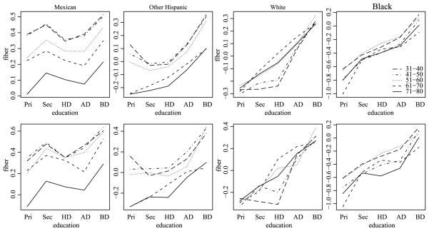
For our data, the F-tests presented in Table 2 indicate strong evidence that the two- and three-way interactions are not zero. Based on these results, standard practice would be to retain the full model and describe the interaction patterns via various contrasts of cell sample means. Often this is done by visual examination of interaction plots, that is, plots of cell means by various combinations of factors. For example, Figure 1 gives the age by education interaction plots for each of the four ethnicity groups. The three-way interaction between ethnicity, age and education can be described as the inconsistency of the two-way interactions across levels of ethnicity. Visually, there is some indication that Mexican respondents have a different age by education interaction than the other ethnicities, but it is difficult to say anything more specific. Indeed, it is difficult to even describe the two-way interactions, due to the high variability of the cell sample means.

Table 2.

MANOVA testing of interaction terms via Pillai’s trace statistic

	approx F	num df	den df	p-value
Education	11.15	15	6102	<0.01
Ethnicity	18.07	9	6102	<0.01
Age	21.38	12	6102	<0.01
Education:Ethnicity	1.67	36	6102	0.01
Education:Age	1.60	48	6102	0.01
Ethnicity:Age	2.05	36	6102	<0.01
Education:Ethnicity:Age	1.44	144	6102	<0.01

Fig. 1.

Three-way interaction plot of fiber cell means by ethnicity, age and education level.

Much of the heterogeneity in these plots can be attributed to the low sample sizes in many cells and the resulting sampling variability of the cell sample means. A cleaner picture of the three-way interactions could possibly be obtained via cell mean estimates with lower variability. A variety of penalized least squares procedures have been proposed in order to reduce estimate variability and mean squared error (MSE), such as ridge regression and the lasso. Recent variants of these approaches allow for different penalties on ANOVA terms of different orders, including the ASP method of Beran (2005) and grouped versions of the lasso [Friedman, Hastie and Tibshirani (2010), Yuan and Lin (2007)]. Corresponding Bayesian approaches include Bayesian lasso procedures [Genkin, Lewis and Madigan (2007), Park and Casella (2008), Yuan and Lin (2005)] and multilevel hierarchical priors [Cui et al. (2010), Hodges et al. (2007), Park, Gelman and Bafumi (2006), Pittau, Zelli and Gelman (2010)].

While these procedures attain a reduced MSE by shrinking linear model coefficient estimates toward zero, they do not generally take full advantage of the structure that is often present in cross-classified data sets. In the data analysis example above, two of the three factors (age and education) are ordinal, with age being a binned version of a continuous predictor. Considering factors such as these more generally, suppose a categorical factor x is a binned version of some underlying continuous or ordinal explanatory variable x̃ (such as income, age, number of children or education level). If the mean of the response variable y is smoothly varying in the underlying variable x̃, we would expect that adjacent levels of the factor x would have similar main effects and interaction terms. Similarly, for nonordinal factors (such as ethnic group or religion) it is possible that two levels represent similar populations, and thus may have similar main effects and interaction terms as well. We refer to such similarities across the orders of the effects as order consistent interactions.

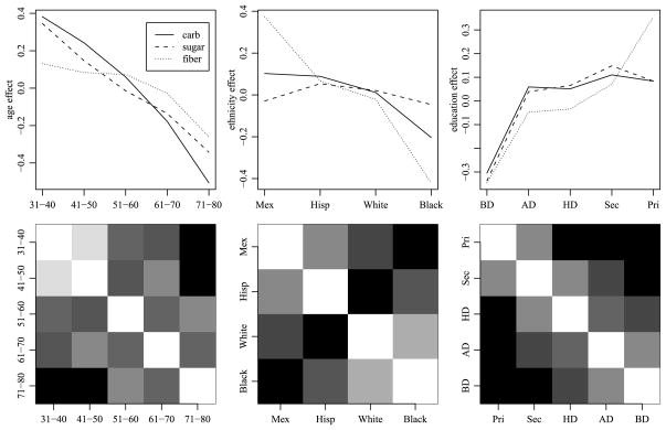
Returning to the NHANES data, Figure 2 summarizes the OLS estimates of the main effects and two-way interactions for the three outcome variables (carbohydrates, sugar and fiber). Not surprisingly, the main effects for the ordinal factors (age and education) are “smooth,” in that the estimated main effect for a given level is generally similar to the effect for an adjacent level. Additionally, some similarities among the ethnic groups appear consistent across the three outcome variables. To assess consistency of such similarities between main effects and two-way interactions, we computed correlations of parameter estimates for these effects between levels of each factor. For example, there are 3 × 10 = 30 main-effect and two-way interaction estimates involving each level of age: For each of the three outcome variables, there is 1 main-effect estimate for each age level, 4 estimates from the age by ethnicity interaction and 5 estimates from the age by education interaction. We compute a correlation matrix for the five levels of age based on the resulting 30 × 5 matrix of parameter estimates, and similarly compute correlations among levels of ethnicity and among levels of education. The second row of Figure 2 gives grayscale plots of these correlation matrices. The results suggest some degree of order consistent interactions: For the ordinal factors, the highest correlations are among adjacent pairs. For the ethnicity factor, the results suggest that, on average, the effects for the Mexican category are more similar to the Hispanic (not Mexican) category than to the other ethnic categories, as we might expect.

Fig. 2.

Plots of main effects and interaction correlations for the three outcome variables (carbohydrates, sugar and fiber). The first row of plots gives OLS estimates of the main effects for each factor. The second row of plots gives correlations of effects between levels of each factor, with white representing 1 and black representing −1. The interactions are calculated based on OLS estimates of the main effects and two-way interactions of each factor.

The OLS estimates of the main effects and three-way interactions presented above, along with the fact that two of the three factors are ordinal, suggest the possibility of order consistent interactions among the array of population cell means. More generally, order consistent interactions may be present in a variety of data sets encountered in the social and health sciences, especially those that include ordinal factors, or factors for which some of the levels may represent very similar populations. In this paper, we propose a novel class of hierarchical prior distributions over main effects and interaction arrays that can adapt to the presence of order consistent interactions. The hierarchical prior distribution provides joint estimates of a covariance matrix for each factor, along with the factor main effects and interactions. Roughly speaking, the covariance matrix for a given factor is estimated from the main effects and interactions in which the factor appears. Conversely, an estimate of a factor’s covariance matrix can assist in the estimation of higher-order interactions, for which data information is limited. We make this idea more formal in the next section, where we construct our prior distribution from a set of related array normal distributions with separable covariance structures [Hoff (2011)] and provide a Markov chain Monte Carlo algorithm for inference under this prior. In Section 3 we provide a simulation study comparing estimation under our proposed prior to some standard estimators. As expected, our approach outperforms others when the data exhibit order consistent interactions. Additionally, for data lacking any interactions, our approach performs comparably to the OLS estimates obtained from the additive model (i.e., the oracle estimator). In Section 4 we extend this methodology to MANOVA models in order to analyze the multivariate NHANES data presented above. In addition to estimates of main effects and interactions, our analysis provides measures of similarity between levels of each of the factors. We conclude in Section 5 with a summary of our approach and a discussion of possible extensions.

2. A hierarchical prior for interaction arrays

In this section we introduce the hierarchical array (HA) prior and present a Markov chain Monte Carlo (MCMC) algorithm for posterior approximation and parameter estimation. The HA prior is constructed from several semi-conjugate priors, and so the MCMC algorithm can be based on a straightforward Gibbs sampling scheme.

2.1. The hierarchical array prior

For notational convenience we consider the case of three categorical factors, and note that the HA prior generalizes trivially to accommodate a greater number of factors. Suppose the three categorical factors have levels {1, …, m₁}, {1, …,m₂} and {1, …,m₃}, respectively. The standard ANOVA model for a three-way factorial data set is

$$\begin{array}{l}{y}_{\mathit{ijkl}}=\mu +a_i+b_j+c_k+{(ab)}_{ij}+{(ac)}_{ik}+{(bc)}_{jk}+{(\mathit{abc})}_{\mathit{ijk}}+{\epsilon }_{\mathit{ijkl}},\\ \{{\epsilon }_{\mathit{ijkl}}\}~\mathrm{i}.\mathrm{i}.\mathrm{d}.\text{normal}(0,{\sigma }^2).\end{array}$$ (1)

Let a denote the m₁ × 1 vector of main effects for the first factor, (ab) denote the m₁ × m₂ matrix describing the two-way interaction between the first two factors, (abc) denote the m₁ × m₂ × m₃ three-way interaction array, and let b, c, (ac) and (bc) be defined similarly. Bayesian inference for this model proceeds by specifying a prior distribution for the ANOVA decomposition θ = {μ, a, b, c, (ab), (ac), (bc), (abc)} and the error variance σ².

As described in the Introduction, if two levels of a factor represent similar populations, we would expect that coefficients of the decomposition involving these two levels would have similar values. For example, suppose levels i₁ and i₂ of the first factor correspond to similar populations. We might then expect a_i1 to be close to a_i2, the vector {(ab)_i1,j, j = 1, …, m₂} to be close to the vector {(ab)_i2,j, j = 1, …, m₂}, and so on. We represent this potential similarity between levels of the first factor with a covariance matrix Σ_a, and consider a mean zero prior distribution on the ANOVA decomposition such that

$$\begin{array}{l}\text{Cov}[a]=\mathrm{E}[{aa}^T]={\mathrm{\sum }}_a,\\ \mathrm{E}[(ab){(ab)}^T]=k_{ab}{\mathrm{\sum }}_a,\\ \mathrm{E}[(ac){(ac)}^T]=k_{ac}{\mathrm{\sum }}_a,\\ \mathrm{E}[{(\mathit{abc})}_{(1)}{(\mathit{abc})}_{(1)}^T]=k_{\mathit{abc}}{\mathrm{\sum }}_a,\end{array}$$

where k_ab, k_ac and k_abc are scalars. Here, (abc)₍₁₎ is the matricization of the array (abc), which converts the m₁ × m₂ × m₃ array into an m₁ × (m₂m₃) matrix by adjoining the m₃ matrices of dimension m₁ × m₂ that form the array (abc) [Kolda and Bader (2009)]. To accommodate similar structure for the second and third factors, we propose the following prior covariance model for the main effects and interaction terms:

$$\begin{array}{l}\hfill \text{Cov}[a]={\mathrm{\sum }}_a,\text{Cov}[b]={\mathrm{\sum }}_b,\text{Cov}[c]={\mathrm{\sum }}_c\hfill \\ \text{Cov}[\text{vec}(ab)]={\mathrm{\sum }}_b\otimes {\mathrm{\sum }}_a/{\gamma }_{ab},\text{Cov}[\text{vec}(bc)]={\mathrm{\sum }}_c\otimes {\mathrm{\sum }}_b/{\gamma }_{bc},\\ \text{Cov}[\text{vec}(ac)]={\mathrm{\sum }}_c\otimes {\mathrm{\sum }}_a/{\gamma }_{ac}\text{Cov}[\text{vec}(\mathit{abc})]={\mathrm{\sum }}_c\otimes {\mathrm{\sum }}_b\otimes {\mathrm{\sum }}_a/{\gamma }_{\mathit{abc}},\end{array}$$

where “⊗” is the Kronecker product. The covariance matrices Σ_a, Σ_b and Σ_c represent the similarities between the levels of each of the three factors, while the scalars γ_ab, γ_ac, γ_bc, γ_abc represent the relative (inverse) magnitudes of the interaction terms as compared to the main effects. Further specifying the priors on the ANOVA decomposition parameters as being mean-zero and Gaussian, the prior on a is then the multivariate normal distribution N_m1(0, Σ_a), and the prior on vec(ab) is N_m1m2 (0, Σ_b ⊗ Σ_a/γ_ab). This latter distribution is sometimes referred to as a matrix normal distribution [Dawid (1981)]. Similarly, the prior on vec(abc) is N_m1m2m3 (0, Σ_c ⊗ Σ_b ⊗ Σ_a/γ_abc), which has been referred to as an array normal distribution [Hoff (2011)].

In classical ANOVA decompositions, it is common to impose an identifiability constraint on the different effects. In a Bayesian analysis it is possible to place priors over identifiable sets of parameters, but this is cumbersome and not frequently done in practice [Gelman and Hill (2007), Kruschke (2011)]. The priors we propose for the effects in the ANOVA decomposition in this article induce a prior over the cell means, which are identifiable. These priors have an intuitive interpretation and do not negatively affect the convergence of MCMC chains generated by the proposed procedure as can be seen in the Simulation and Application sections.

In most data analysis situations the similarities between the levels of a given factor and magnitudes of the interactions relative to the main effects will not be known in advance. We therefore consider a hierarchical prior so that Σ_a, Σ_b, Σ_c and the γ-parameters are estimated from the data. Specifically, we use independent inverse-Wishart prior distributions for each covariance matrix, for example, ${\mathrm{\sum }}_a~\text{inverse}-\text{Wishart}({\eta }_{a0},S_{a0}^{-1})$, and gamma priors for the γ-parameters, for example, ${\gamma }_{ab}~\text{gamma}(v_{ab0}/2,{\tau }_{ab0}^2/2)$, where η_a, S_a, ν_ab0 and ${\tau }_{ab0}^2$ are hyperparameters to be specified (some default choices for these parameters are discussed at the end of this section). This hierarchical prior distribution can be viewed as an adaptive penalty, which allows for sharing of information across main effects and interaction terms. For example, estimates of the three-way interaction will be stabilized by the covariance matrix Σ_c ⊗ Σ_b ⊗ Σ_a, which in turn is influenced by similarities between levels of the factors that are consistent across the main effects, two-way and three-way interactions.

2.2. Posterior approximation

Due to the semi-conjugacy of the HA prior, posterior approximation can be obtained from a straightforward Gibbs sampling scheme. Under this scheme, iterative simulation of parameter values from the corresponding full conditional distributions generates a Markov chain having a stationary distribution equal to the target posterior distribution. For computational simplicity, we consider the case of a balanced data set in which the sample size in each cell is equal to some common value n, in which case the data can be expressed as an m₁ × m₂ × m₃ × n four-way array Y. A modification of the algorithm to accommodate unbalanced data is discussed in the next subsection.

Derivation of the full conditional distributions of the grand mean μ and the error variance σ² are completely standard: Under a $N({\mu }_0,{\tau }_0^2)$ prior for μ, the corresponding full conditional distribution is $N({\mu }_1,{\tau }_1^2)$, where ${\tau }_1^2={(1/{\tau }_0^2+{nm}_1{m}_2{m}_3/{\sigma }^2)}^{-1}$ and ${\mu }_1={\tau }_1^2({\mu }_0/{\tau }_0^2+{nm}_1{m}_2{m}_3\overline{r}/{\sigma }^2)$, where r̄ = Σ_ijkl (y_ijkl − [a_i + b_j + c_k + (ab)_ij + (ac)_ik + (bc)_jk + (abc)_ikj])/n. Under an $\text{inverse}-\text{gamma}(v_0/2,v_0{\sigma }_0^2/2)$ prior distribution, the full conditional distribution of σ² is an $\text{inverse}-\text{gamma}(v_1/2,v_1{\sigma }_1^2/2)$ distribution, where ν₁ = ν₀ + nm₁m₂m₃, $v_1{\sigma }_1^2=v_0{\sigma }_0^2+{\sum }_{\mathit{ijkl}}{(y_{\mathit{ijkl}}-{\mu }_{\mathit{ijk}})}^2$ and μ_ijk = μ + a_i + b_j + c_k + (ab)_ij + (ac)_ik + (bc)_jk + (abc)_ikj. Derivation of the full conditional distributions of parameters other than μ and σ² is straightforward, but slightly nonstandard due to the use of matrix and array normal prior distributions for the interaction terms. In what follows, we compute the full conditional distributions for a few of these parameters. Full conditional distributions for the remaining parameters can be derived in an analogous fashion.

Full conditionals of a and (abc)

To identify the full conditional distribution of the vector a of main effects for the first factor, let

$$\begin{array}{l}{r}_{\mathit{ijkl}}=y_{\mathit{ijkl}}-(\mu +b_j+c_k+{(ab)}_{ij}+{(ac)}_{ik}+{(bc)}_{jk}+{(\mathit{abc})}_{\mathit{ijk}})\\ =a_i+{\epsilon }_{\mathit{ijkl}},\end{array}$$

that is, r_ijkl is the “residual” obtained by subtracting all effects other than a from the data. Since {ε_ijkl } ~ i.i.d. normal(0, σ², we have

$$p(Y\mid \theta ,{\sigma }^2){\propto }_{a}exp\left\{-\frac{m_2{m}_{3}n}{2{\sigma }^2}(a^{T}a-2a^T\overline{r})\right\},$$

where r̄ = (r̄₁, …,r̄_m1) with r̄_i = Σ_jkl r_ijkl/(m₂m₃n), θ = {μ, a, b, c, (ab), (ac), (bc), (abc)} and “∝_a” means “proportional to as a function of a.” Combining this with the N_m1 (0, Σ_a) prior density for a, we have

$$p(a\mid Y,{\theta }_{-a},{\sigma }^2,{\mathrm{\sum }}_a){\propto }_{a}exp\left(-\frac{m_2{m}_{3}n}{2{\sigma }^2}[a^{T}a-2a^T\overline{r}]-\frac{1}{2}{a}^T{\mathrm{\sum }}_a^{-1}a\right)$$

and so the full conditional distribution of a is multivariate normal with

$$\begin{array}{l}\text{Var}[a\mid Y,{\theta }_{-a},{\sigma }^2,{\mathrm{\sum }}_a]={({\mathrm{\sum }}_a^{-1}+I{m}_2{m}_{3}n/{\sigma }^2)}^{-1},\\ \text{Exp}[a\mid Y,{\theta }_{-a},{\sigma }^2,{\mathrm{\sum }}_a]={({\mathrm{\sum }}_a^{-1}+I{m}_2{m}_{3}n/{\sigma }^2)}^{-1}\overline{r}\times (m_2{m}_{3}n/{\sigma }^2),\end{array}$$

where I is the m₁ × m₁ identity matrix.

Derivation of the full conditional distributions for the interaction terms is similar. For example, to obtain the full conditional distribution of (abc), let r_ijkl be the residual obtained after subtracting all other components of θ from the data, so that r_ijkl = (abc)_ijk + ε_ijkl. Let r̄ be the three-way array of cell means of {r_ijkl }, so that r̄_ijk = Σ_l r_ijkl/n. Combining the likelihood in terms of r̄ with the N_m1m2m3 (0, Σ_c ⊗ Σ_b ⊗ Σ_a/γ_abc) prior density for vec(abc) gives

$$\begin{array}{l}p((\mathit{abc})\mid Y,{\sigma }^2,{\mathrm{\sum }}_a,{\mathrm{\sum }}_b,{\mathrm{\sum }}_c,{\gamma }_{\mathit{abc}},{\theta }_{-(\mathit{abc})})\\ {\propto }_{(\mathit{abc})}exp\left(-\frac{n}{2}[\text{vec}{(\mathit{abc})}^T\text{vec}(\mathit{abc})-2\text{vec}{(\mathit{abc})}^T\text{vec}(\overline{r})]\right)\\ \times exp\left(-\frac{1}{2}\text{vec}{(\mathit{abc})}^T{({\mathrm{\sum }}_c\otimes {\mathrm{\sum }}_b\otimes {\mathrm{\sum }}_c/{\gamma }_{\mathit{abc}})}^{-1}\text{vec}(\mathit{abc})\right)\end{array}$$

and so vec(abc) has a multivariate normal distribution with variance and mean given by

$$\begin{array}{l}\text{Var}[\text{vec}(\mathit{abc})\mid Y,{\theta }_{-(\mathit{abc})},{\sigma }^2,{\mathrm{\sum }}_a,{\mathrm{\sum }}_b,{\mathrm{\sum }}_c,{\gamma }_{\mathit{abc}}]={({({\mathrm{\sum }}_c\otimes {\mathrm{\sum }}_b\otimes {\mathrm{\sum }}_a/{\gamma }_{\mathit{abc}})}^{-1}+In/{\sigma }^2)}^{-1},\\ \mathrm{E}[\text{vec}(\mathit{abc})\mid Y,{\theta }_{-(\mathit{abc})},{\sigma }^2,{\mathrm{\sum }}_a,{\mathrm{\sum }}_b,{\mathrm{\sum }}_c,{\gamma }_{\mathit{abc}}]={({({\mathrm{\sum }}_c\otimes {\mathrm{\sum }}_b\otimes {\mathrm{\sum }}_a/{\gamma }_{\mathit{abc}})}^{-1}+In/{\sigma }^2)}^{-1}\text{vec}(\overline{r})\times n/{\sigma }^2.\end{array}$$

Full conditional distributions for the remaining effects can be derived analogously.

Full conditional of Σ_a

The parameters in the ANOVA decomposition whose priors depend on Σ_a are a, (ab), (ac) and (abc). For example, the prior density of (ab) given Σ_a, Σ_b and γ_ab can be written as

$$\begin{array}{l}p((ab)\mid {\mathrm{\sum }}_a,{\mathrm{\sum }}_b,{\gamma }_{ab})={\mid 2\pi {\mathrm{\sum }}_b\otimes {\mathrm{\sum }}_a/{\gamma }_{ab}\mid }^{-1/2}\\ \times exp(-\text{vec}{(ab)}^T{[{\mathrm{\sum }}_b\otimes {\mathrm{\sum }}_a/{\gamma }_{ab}]}^{-1}\text{vec}(ab)/2)\\ {\propto }_{{\mathrm{\sum }}_a}{\mid {\mathrm{\sum }}_a\mid }^{-m_2/2}\text{etr}(-{\mathrm{\sum }}_a^{-1}{\gamma }_{ab}{(ab)}^T{\mathrm{\sum }}_b^{-1}(ab)/2)\\ ={\mid {\mathrm{\sum }}_a\mid }^{-m_2/2}\text{etr}(-{\mathrm{\sum }}_a^{-1}{S}_{ab}/2),\end{array}$$

where $S_{ab}={\gamma }_{ab}{(ab)}^T{\mathrm{\sum }}_b^{-1}(ab)$ and etr(A) = exp{trace(A)} for a square matrix A. Similarly, the priors for a, (ac) and (abc) are proportional to ${\mid {\mathrm{\sum }}_a\mid }^{-d_i/2}\times \text{etr}(-{\mathrm{\sum }}_a^{-1}{S}_i/2)$ (as a function of Σ_a) for i ∈ {a, ac, abc} where

$$\begin{array}{l}{S}_a={aa}^T,\\ S_{ac}={\gamma }_{ac}{(ac)}^T{\mathrm{\sum }}_c^{-1}(ac),\\ S_{\mathit{abc}}={\gamma }_{\mathit{abc}}{(\mathit{abc})}_{(1)}{({\mathrm{\sum }}_c\otimes {\mathrm{\sum }}_b)}^{-1}{(\mathit{abc})}_{(1)},\end{array}$$

and d_a = d_ac = m₃ and d_abc = m₂m₃. The $\text{inverse}-\text{Wishart}({\eta }_{a0},S_{a0}^{-1})$ prior density for Σ_a can also be written in a similar fashion: it is proportional to ${\mid {\mathrm{\sum }}_a\mid }^{-({\eta }_{a0}+m_1+1)/2}\text{etr}(-{\mathrm{\sum }}_a^{-1}{S}_{a0}/2)$. Multiplying together the prior densities for a, (ab), (ac), (abc) and Σ_a and simplifying by the additivity of exponents and the linearity of the trace gives

$$p({\mathrm{\sum }}_a\mid \theta ,{\mathrm{\sum }}_b,{\mathrm{\sum }}_c,\gamma )\propto {\mid {\mathrm{\sum }}_a\mid }^{-(1+m_1+{\eta }_{a0}+1+m_2+m_3+m_2{m}_3)/2}\times \text{etr}(-{\mathrm{\sum }}_a^{-1}(S_{a0}+S_a+S_{ab}+S_{ac}+S_{\mathit{abc}})/2).$$

It follows that the full conditional distribution of Σ_a is $\text{inverse}-\text{Wishart}({\eta }_{a1},S_{a1}^{-1})$, where η_a1 = η_a0 + (1 + m₂ + m₃ + m₂m₃) and S_a1 = S_a0 + S_a + S_ab + S_ac + S_abc. The full conditional expectation of Σ_a is therefore S_a1/(η_a1 − m₁ − 1), which combines several estimates of the similarities among the levels of the first factor, based on the main effects and the interactions.

Full conditional of γ_abc

The full conditional distribution of γ_abc depends only on the (abc) interaction term. The normal prior for (abc) can be written as

$$p((\mathit{abc})\mid {\mathrm{\sum }}_a,{\mathrm{\sum }}_b,{\mathrm{\sum }}_c,{\gamma }_{\mathit{abc}}){\propto }_{{\gamma }_{\mathit{abc}}}{\gamma }_{\mathit{abc}}^{m_1{m}_2{m}_3/2}exp\{-{\gamma }_{\mathit{abc}}\text{vec}{(\mathit{abc})}^T{[{\mathrm{\sum }}_c\otimes {\mathrm{\sum }}_b\otimes {\mathrm{\sum }}_a]}^{-1}\text{vec}{(\mathit{abc})}^T/2\}.$$

Combining this density with a $\text{gamma}(v_{\mathit{abc}0}/2,{\tau }_{\mathit{abc}0}^2/2)$ prior density yields a full conditional for γ_abc that is $\text{gamma}(v_{\mathit{abc}1}/2,{\tau }_{\mathit{abc}1}^2/2)$, where

$$\begin{array}{l}{v}_{\mathit{abc}1}=v_{\mathit{abc}0}+m_1{m}_2{m}_3,\\ {\tau }_{\mathit{abc}1}^2={\tau }_{\mathit{abc}0}^2+\text{vec}{(\mathit{abc})}^T{[{\mathrm{\sum }}_c\otimes {\mathrm{\sum }}_b\otimes {\mathrm{\sum }}_a]}^{-1}\text{vec}(\mathit{abc}).\end{array}$$

2.3. Balancing unbalanced designs

For most survey data we expect the sample sizes {n_ijk } to vary across combinations of factors. As a result, the full conditional distributions of the ANOVA decomposition parameters are more difficult to compute. For example, the conditional variance of the three-way interaction vec(abc) changes from (γ_abc(Σ_c ⊗ Σ_b ⊗ Σ_a)⁻¹ + In/σ²)⁻¹ in the balanced case to (γ_abc(Σ_c ⊗ Σ_b ⊗ Σ_a)⁻¹ + D/σ²)⁻¹ in the general case, where D is a diagonal matrix with diagonal elements vec({n_ijk }). Even for moderate numbers of levels of the factors, the matrix inversions required to calculate the full conditional distributions in the unbalanced case can slow down the Markov chain considerably. As an alternative, we propose the following data augmentation procedure to “balance” an unbalanced design. Let Ȳ^o be the three-way array of cell means based on the observed data, that is, ${\overline{y}}_{\mathit{ijk}}^o=\sum y_{\mathit{ijkl}}/n_{\mathit{ijk}}$. Letting n = max({n_ijk }), for each cell ijk with sample size n_ijk < n and at each step of the Gibbs sampler, we impute a cell mean based on the “missing” n − n_ijk observations as ${\overline{y}}_{\mathit{ijk}}^m~\text{normal}({\mu }_{\mathit{ijk}},{\sigma }^2/[n_{max}-n_{\mathit{ijk}}])$, where μ_ijk is the population mean for cell ijk based on the current values of the ANOVA decomposition parameters. We then combine ${\overline{y}}_{\mathit{ijk}}^o$ and ${\overline{y}}_{\mathit{ijk}}^m$ to form the “full sample” cell mean ${\overline{y}}_{\mathit{ijk}}^f=(n_{\mathit{ijk}}{\overline{y}}_{\mathit{ijk}}^o+(n-n_{\mathit{ijk}}){\overline{y}}_{\mathit{ijk}}^m)/n$. This array of cell means provides the sufficient statistics for a balanced data set, for which the full conditional distributions derived above can be used.

2.4. Setting hyperparameters

In the absence of detailed prior information about the parameters, we suggest using a modified empirical Bayes approach to hyperparameter selection based on the maximum likelihood estimates (MLEs) of the error variance and mean parameters. Priors for μ and σ² can be set as unit information priors [Kass and Wasserman (1995)], whereby hyperparameters are chosen so that the prior means are near the MLEs but the prior variances are set to correspond roughly to only one observation’s worth of information. For the covariance matrices Σ_a, Σ_b and Σ_c, recall that the prior for the main effect a of the first factor is N_m1 (0, Σ_a). Based on this, we choose the prior for Σ_a to be $\text{inverse}-\text{Wishart}(v_{a0},S_{a0}^{-1})$ with ν_a0 = m₁ + 2 and S_a0 = ||a||²I_m1/m₁, where â is the MLE of a and ||â|| is the L₂ norm of â. Under this prior, E[tr(Σ_a)] = ||â||², and so the scale of the prior matches the empirical estimates. Finally, the γ-parameters can be set analogously, using diffuse gamma priors but centered around values to match the magnitude of the OLS estimates of the interaction terms they correspond to, relative to the magnitude of the main effects. For example, in the next section we use a $\text{gamma}(v_{ab0}/2,{\tau }_{ab0}^2/2)$ prior for γ_ab in which ν_ab0 = 1 and ${\tau }_{ab0}^2={\Vert \widehat{a}\Vert }^2{\Vert \widehat{b}\Vert }^2/{\Vert (\widehat{ab})\Vert }^2$, where â, b̂ and ( $\widehat{ab}$) are the OLS estimates.

The above procedure can be modified to accommodate an incomplete design, where not all the OLS estimates are available for a complete model. For example, in a two-way example, if exactly one cell is empty, then the OLS estimates are available for all effect levels except for the two-way interaction for the missing cell. Abusing notation a bit, let ||( $\widehat{ab}$)|| be the L₂ norm of available OLS estimates for the two-way interaction. There are m₁m₂ − 1 of these. Note that this will likely underestimate ||(ab)||, as it is missing the component contributed by the missing cell. To correct for this underestimate, we propose the following modification for setting the hyperparameters: ${\Vert (\stackrel{\sim }{ab})\Vert }^2=\Vert (\widehat{ab})\Vert (m_1{m}_2)/(m_1{m}_2-1)$. The choice of ${\tau }_{ab0}^2$ above becomes ${\Vert \widehat{a}\Vert }^2{\Vert \widehat{b}\Vert }^2/{\Vert (\stackrel{\sim }{ab})\Vert }^2$.

3. Simulation study

This section presents the results of four simulation studies comparing the HA prior to several competing approaches. The first simulation study uses data generated from a means array that exhibits order consistent interactions. Estimates based on the HA prior outperform standard OLS estimates as well as estimates from a standard Bayesian (SB) approach as in Gelman (2005), and is also related to a grouped version of the lasso procedure [Yuan and Lin (2006)]. The second simulation study uses data from a means array that exhibits “order inconsistent” interactions, that is, interactions without consistent similarities in parameter values between levels of a factor. In this case the HA prior still outperforms the OLS and standard Bayes approaches, although not by as much as in the presence of order consistent interactions. In the third simulation we study the Bayes risk of the HA procedure when data is generated directly from the SB prior. Unlike the second simulation study, where interactions were “order inconsistent” but had potential similarities, in this case all effects were completely independent and so the oracle SB approach that imposes independence on the interaction effects outperforms HA, though not by much. The fourth simulation study uses data from a means array that has an exact additive decomposition, that is, there are no interactions. The HA prior procedure again outperforms the standard Bayes and OLS approaches, although it does not do as well as OLS and Bayes oracle estimators that assume the correct additive model.

The Markov chain Monte Carlo algorithms were implemented using the R statistical programming language on a computer with a 2.5 GHz processor. The additive Bayes approach is significantly faster than the other two Bayesian procedures since it contains the fewest parameters. The other two procedures are comparable, but with SB being somewhat faster than HA on average. Specifically, for the simulations conducted below, SB ran an estimated 17% faster than HA, which had a run time on the order of 16 minutes per data set (depending on sample size). The overall runtime improves by almost 50% if the data set is balanced.

3.1. Data with order consistent interactions

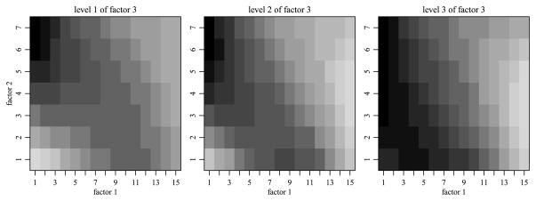
The data in this simulation study is generated from a model where the means array exhibits order consistent interactions. The dimensions of the means array M were chosen to be m₁ × m₂ × m₃ = 15 × 7 × 3, which could represent, for example, the number of categories we might have for age, education level and political affiliation in a cross-classified survey data set. The means array was generated from a cubic function of three variables that was then binned. Figure 3 plots the mean array across the third factor, demonstrating the nonadditivity present in M. By decomposing M into the main, two-way and three-way effects in the same manner as described in Section 2, we can summarize the nonadditivity of M through the magnitudes of the different sums of squares. The magnitudes of the main effects, given by the squared L₂ norm of the effects, ||a||²/m₁, ||b||²/m₂ and||c||²/m₃, are 5.267, 0.012, 0.004, respectively. Those of the two-way interactions ||ab||²/(m₁m₂), ||ac||²/(m₁m₃) and ||bc||²/(m₂m₃) are 1.365, 1.312 and 0.384, and the magnitude of the three-way interaction ||abc||²/(m₁m₂m₃) is 0.474. For each sample size {400, 1000, 5000, 10,000}, we simulated 50 data sets using the mean array M and independent standard normal errors. In order to make a comparison to OLS possible, we first allocated one observation to each cell of the means array. We then distributed the remaining observations uniformly at random (with replacement) among the cells of the means array. This leads to a complete but potentially unbalanced design. The average number of observations per cell under the sample sizes {400, 1000, 5000, 10,000} was {1.3, 3.2, 15.9, 31.7}.

Fig. 3.

The means array M across levels of the third factor.

For each simulated data set we obtained estimates under the HA prior (using the hyperparameter specifications described in Section 2.4), as well as ordinary least squares estimates (OLS) and posterior estimates under a standard Bayesian prior (SB). The SB approach is essentially a simplified version of the HA prior in which the parameter values are conditionally independent given the hyperparameters: $\{a_i\}~\mathrm{i}.\mathrm{i}.\mathrm{d}.\mathrm{N}(0,{\sigma }_a^2),\{{(ab)}_{ij}\}~\mathrm{i}.\mathrm{i}.\mathrm{d}.\mathrm{N}(0,{\sigma }_{ab}^2)$ and $\{{(\mathit{abc})}_{\mathit{ijk}}\}~\mathrm{i}.\mathrm{i}.\mathrm{d}.(0,{\sigma }_{\mathit{abc}}^2)$, and similarly for all other main effects and interactions. To facilitate comparison to the HA prior, the hyperpriors for these σ²-parameters are the same as the hyperpriors for the inverses of the γ-parameters in the HA approach. As a result, this standard Bayes prior can be seen as the limit of a sequence of HA priors where the inverse-Wishart prior distributions for the Σ-matrices converge to point masses on the identity matrices of the appropriate dimension.

For each simulated data set, the Gibbs sampler described in Section 2 was run for 11,000 iterations, the first 1000 of which were dropped to allow for convergence to the stationary distribution. Parameter values were saved every 10th scan, resulting in 1000 Monte Carlo samples per simulation. Starting values for all the mean effects were set to zero and all variances set to identity matrices of the proper dimensions. We examined the convergence and autocorrelation of the marginal samples of the parameters in each procedure. Since the number of parameters is large, we present the results of Geweke’s z-test and estimates of the effective sample size for the error variance σ², as it provides a parsimonious summary of the convergence results. The minimum effective sample size across all simulations was 233 out of the 1000 recorded scans, and the average effective sample size was 895. Geweke’s z-statistic was less than 2 in absolute value in 93, 93, 97 and 95 percent of the Markov chains for the four sample sizes (with the percentages being identical for both Bayesian methods). While the cases in which |z| > 2 were not extensively examined, it is assumed that running the chain longer would have yielded improved estimation.

For each simulated data set, the posterior mean estimates M̂_HA and M̂_SB were obtained by averaging their values across the 1000 saved iterations of the Gibbs sampler. The average squared error (ASE) of estimation was calculated as ASE(M̂) = ||M̂ − M||²/(m₁m₂m₃), where M is the means array that generated the data. These values were then compared across the three approaches. The left panel of Figure 4 demonstrates that the SB estimator provided a reduction in ASE when compared to the OLS estimator for all data sets with sample sizes 400 and 1000, 96% of the data sets with sample size 5000 and 90% of data sets with sample size 10,000. The second panel demonstrates that the HA estimator provides a substantial further reduction in ASE for all data sets. As we would expect, the reduction in ASE is dependent on the sample size and decreases as the sample size increases.

Fig. 4.

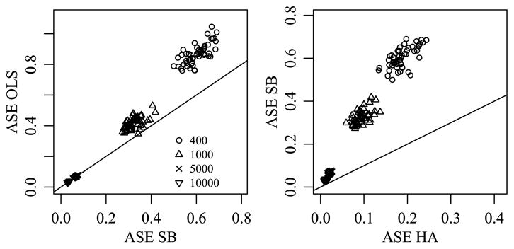
Comparison of ASE for different estimation methods when the true means array exhibits order consistent interactions.

These results are not surprising: By estimating the variances ${\sigma }_a^2,{\sigma }_{ab}^2$, etc. from the data, the SB approach provides adaptive shrinkage and so we expect these SB estimates to outperform the OLS estimates in terms of ASE. However, the SB approach does not use information on the similarity among the levels of an effect, and so its estimation of higher order interactions relies on the limited information available directly in the corresponding sufficient statistics. As such, we expect the SB estimates to perform less well than the HA estimates, which are able to borrow information from well-estimated main effects and low-order interactions to assist in the estimation of higher-order terms for which data information is limited.

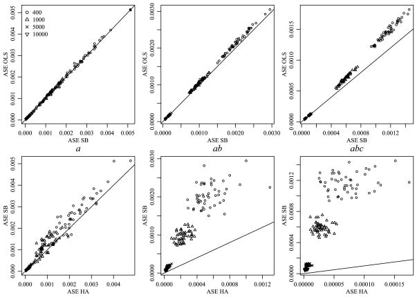
This behavior is further illustrated in Figure 5 that provides an ASE comparison for the effects in the decomposition of the means array. To produce these plots, we decomposed each estimated means array and considered the ASE for each effect when compared to the decomposition of the true means array. It is immediate that the gains in ASE are primarily from improved estimation of the higher order interaction terms. The top row of Figure 5 demonstrates that the SB estimator performs at least as well as the OLS estimator in terms of ASE for the main effect a, and provides a detectable reduction in ASE for two- and three-way interactions. The reduction in ASE for the higher order terms is due to the shrinkage provided by SB. The second row of Figure 5 demonstrates that the HA estimator provides a moderate reduction in ASE for the main effect a and a substantial further reduction in ASE for the higher order terms. This is exactly the behavior we expect, as the HA procedure is able to borrow information from lower order terms in order to further shrink higher order interactions. We have also evaluated the width and coverage of nominal 95% confidence intervals for the cell means. The results for HA and SB are presented in Table 3. The confidence intervals for the entries in the means array were smaller for the HA procedure than for SB, while the coverage was approximately 95% for both.

Fig. 5.

ASE comparisons for the main effect, a two-way interaction and a three-way interaction that involve a are in the three columns, respectively. The first row compares ASE between SB and OLS and the second row compares ASE between HA and SB.

Table 3.

Actual coverage and interval widths of 95% nominal confidence intervals for the cell means as estimated by HA and SB when order consistent interactions are present

OBS	Coverage		Width
	HA	SB	HA	SB
400	0.94	0.93	1.55	3.18
1000	0.93	0.95	1.04	2.32
5000	0.94	0.94	0.49	1.00
10,000	0.95	0.95	0.36	0.70

Recall that the parameters in the mean array M were generated by binning a third-degree polynomial, and were not generated from array normal distributions, that is, the HA prior is “incorrect” as a model for M. Even so, the HA prior is able to capture the similarities between adjacent factor levels, resulting in improved estimation. However, we note that not all of the improvement in ASE achieved by the HA prior should be attributed to the identification of order-consistent interactions. The simulation study that follows suggests some of the performance of the HA prior is due to additional parameter shrinkage provided by the inverse-Wishart distributions on the Σ-matrices.

3.2. Data with order inconsistent interactions

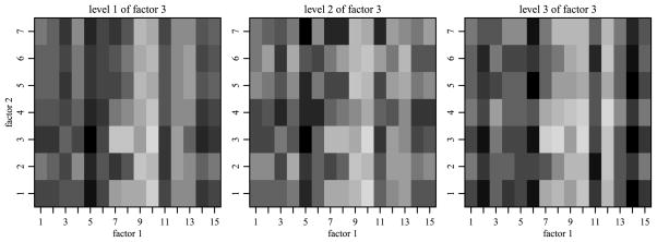
In this subsection we evaluate the HA approach for populations which exhibit interactions that are order inconsistent. The means array M is constructed by taking the means array from Section 3.1, decomposing it into main effects, two- and three-way interactions, permuting the levels of each factor within each effect, and reconstructing a means array. That is, if {a_i : i = 1, …, m₁} is the collection of parameters for the first main effect and {(ab)_ij : i = 1, …, m₁, j = 1, …, m₂} is the collection of parameters for the two-way interaction between the first and second factors in Section 3.1, then {a_π1(i)} and {(ab)_{π2(i) π3(j)}} are the main effect and two-way interaction parameters for the means array in this section, where π₁, π₂ and π₃ are independent permutations. The remaining effects were permuted analogously. Due to this construction, the magnitudes of the main effects, two- and three-way interactions remain the same, but the process becomes less “smooth,” as can be seen in Figure 6.

Fig. 6.

The means array M for the second simulation study, across levels of the third factor.

Again, 50 data sets were generated for each sample size, and estimates M̂_HA, M̂_SB and M̂_OLS were obtained for each data set, where the Bayesian estimates were obtained using the same MCMC approximation procedure as in the previous subsection. Figure 7 compares ASE across the different approaches. The left panel of Figure 7, as with the left panel of Figure 4, demonstrates that the SB estimator provides a reduction in ASE when compared to the OLS estimator. As expected, since neither of these approaches take advantage of the structure of the order consistent interactions, this plot is nearly identical to the corresponding plot in Figure 4.

Fig. 7.

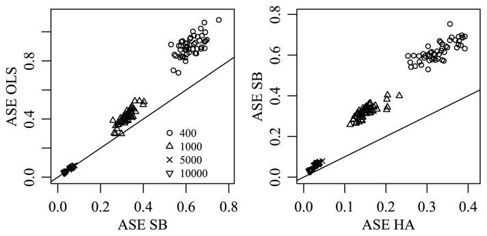
Comparison of ASE for different estimation methods when the true means array exhibits order inconsistent interactions that have the same magnitude as the order consistent interactions of Section 3.1.

The second panel demonstrates that the HA estimator provides a further reduction in ASE for all data sets, although this reduction is less substantial than in the presence of order consistent interactions. The lower ASE of the HA estimates may be initially surprising, as there are no order consistent interactions for the HA prior to take advantage of. We conjecture that the lower ASE is due to the additional shrinkage on the parameter estimates that the inverse-Wishart priors on the Σ-parameters provide. For example, under both the SB and HA priors we have Cov[vec(ab)] = Σ_b ⊗ Σ_a/γ_ab, but under the former the covariance matrices are set to the identity, whereas under the latter they have inverse-Wishart distributions.

As with the previous simulation, we evaluated the width and coverage of nominal 95% confidence intervals for the cell means. The results for HA and SB are presented in Table 4. As in the previous simulation, the coverage for both procedures is approximately 95%. The confidence intervals are wider for SB than for HA, but the differences between the two procedures are much smaller in this simulation as compared to the previous one.

Table 4.

Actual coverage and interval widths of 95% nominal confidence intervals for the cell means as estimated by HA and SB when order inconsistent interactions are present

OBS	Coverage		Width
	HA	SB	HA	SB
400	0.95	0.94	2.26	2.98
1000	0.95	0.95	1.56	2.15
5000	0.96	0.95	0.73	0.98
10,000	0.96	0.94	0.53	0.69

3.3. Data with order inconsistent interactions: Bayes risk

The surprising outcome of the previous section requires further study of the behavior of the HA approach when order inconsistent interactions are present. To get a more complete picture of this behavior, we evaluate the Bayes risk of the procedure when data is generated directly from the SB prior. We construct 200 means arrays M₁, …, M₂₀₀ of the same dimensions as in the previous subsections using the following procedure:

1. Generate γ_a, γ_b, γ_c, γ_ab, γ_ac, γ_bc, ${\gamma }_{\mathit{abc}}\stackrel{\mathrm{i}.\mathrm{i}.\mathrm{d}.}{\sim }\text{gamma}(v/2,{\tau }^2/2)$ with shape paramter ν = 4 and rate parameter τ² = 2. These are the precision components for the 3 main effects, 3 two-way interactions and 1 three-way interaction, respectively.

2. Generate effect levels as follows: {a₁, …, a₁₅} ~ N(0, I/γ_a), {ab_1,1, …, ab_15,7} ~ N(0, I/γ_ab), and similarly for the remaining 5 effects.

3. Combine the effects from (2) into a means array M_i according to equation (1).

For each sample size {400, 1000, 5000, 10,000} we generated 50 data sets, each using a unique means array M_i, in the same manner as in the previous two simulation studies. We obtained estimates M̂_iHA, M̂_iSB and M̂_iOLS for each data set, where the Bayesian estimates were obtained using the same MCMC procedure as in the previous two subsections.

ASE represents the posterior quadratic loss of an estimation procedure for a particular data set, and so by varying the true means array M_i between simulated data sets, we can estimate the Bayes risk of an estimation procedure by taking the average of ASE across simulated data sets. The Bayes risk for the SB procedure is guaranteed to be smaller than that for OLS and HA for all sample sizes and so we report the results of the simulation study as ratios of estimated Bayes risk for SB to the estimated Bayes risk of the other procedures in Table 5. For example, the first entry in the top row of Table 5 states that the Bayes risk for SB is 41% lower than the Bayes risk for the OLS procedure for a sample size of 400. As is expected, the difference in Bayes risk shrinks with increasing sample size for both OLS and HA. The results of this simulation study suggest that even for moderately sized data sets, the relative risk of using the HA procedure when compared to SB is rather small even when all effects are completely independent. Additionally, the posterior estimates of all of the effects in the decomposition of the means array had similar variances under both SB and HA priors. This suggests that using the HA procedure is not detrimental even when the “order consistency” of the interactions cannot be verified.

Table 5.

Ratio of estimated Bayes risk for SB to OLS and HA by sample size

Sample size	400	1000	5000	10,000
OLS	0.59	0.69	0.93	0.97
HA	0.78	0.91	0.97	0.98

3.4. Data without interactions

In this subsection we evaluate the HA approach for populations in which interactions are not present. The data in this simulation is generated from a model where the means array M is exactly additive and was constructed by binning a linear function of three variables. As in the previous simulations, M is of dimension m₁ × m₂ × m₃ = 15 × 7 × 3. The magnitudes of the three main effects are ||a||²/m₁ = 3.0, ||b||²/m₂ = 1.3 and ||c||²/m₃ = 0.3, while all interactions are exactly zero. In addition to the SB and OLS estimators, we compare the HA approach to two “oracle” estimators: the additive model least squares estimator (AOLS) and the Bayes estimator under the additive model (ASB). The prior used by the ASB approach is the same as the SB prior, but does not include terms other than main effects in the model.

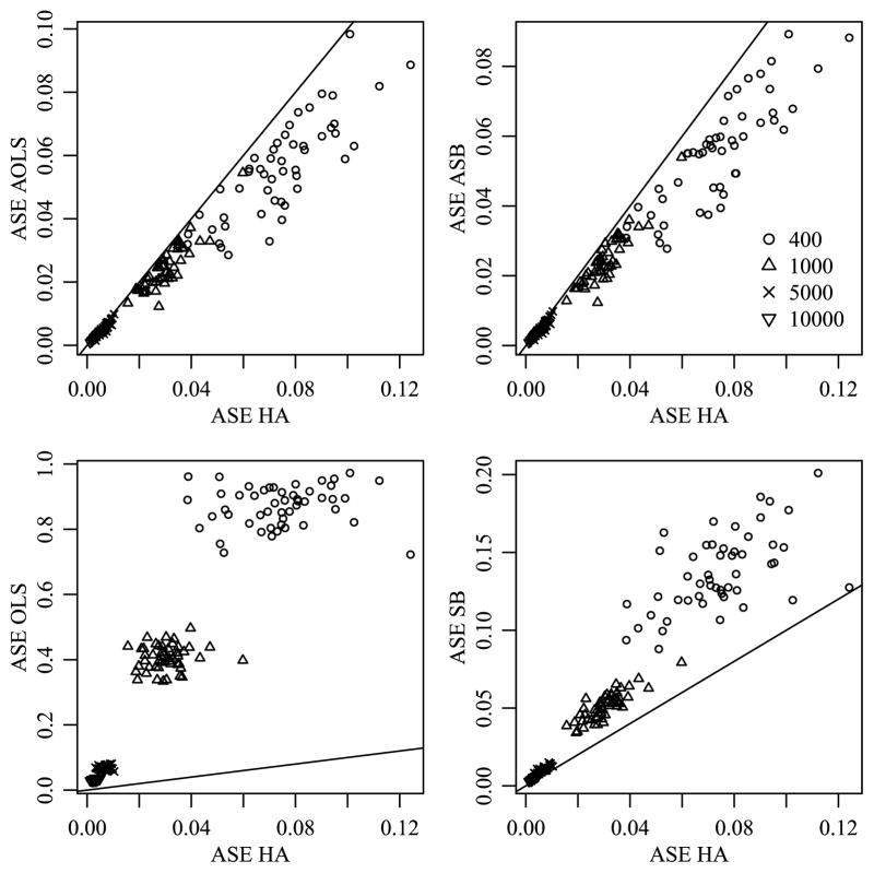
As before, 50 data sets were generated for each sample size, and estimates M̂_HA, M̂_SB, M̂_OLS, M̂_ASB and M̂_AOLS were obtained for each data set, where the Bayesian estimates were obtained using the same MCMC approximation procedure as in the previous two subsections. Some results are shown in Figure 8, which compares ASE across the different approaches. In the top row of Figure 8 we see that the performance of the HA estimates is comparable to but not as good as the oracle least squares and Bayesian estimates in terms of ASE. Specifically, the ASE for the HA estimates is 24.2, 18.6, 20.1 and 17.4 percent higher than for the AOLS estimates for data sets with sample sizes 400, 1000, 5000 and 10,000, respectively. Similarly, the ASE for the HA estimates is 25, 19.7, 20.3 and 17.8 percent higher than for the ASB estimates for data sets with sample sizes 400, 1000, 5000 and 10,000, respectively. However, the bottom row of Figure 8 shows that the HA prior is superior to the other nonoracle OLS and SB approaches that attempt to estimate the interaction terms.

Fig. 8.

Comparison of ASE for different estimation methods when the true means array is additive.

These results, together with those of the last two subsections, suggest that the HA approach provides a competitive method for fitting means arrays in the presence or absence of interactions. When order consistent interactions are present, the HA approach is able to make use of the similarities across levels of the factors, thereby outperforming approaches that cannot adapt to such patterns. Additionally, the HA approach does not appear to suffer when interactions are not order consistent. Finally, in the absence of interactions altogether, the HA approach adapts well, providing estimates similar to those that assume the correct additive model.

4. Analysis of carbohydrate intake

In this section we estimate average carbohydrate, sugar and fiber intake by education, ethnicity and age using the HA procedure described in Section 2. Our estimates are based on data from 2134 males from the US population, obtained from the 2007–2008 NHANES survey. Nutrient intake is self reported on two nonconsecutive days. Each day’s data concerns food and beverage intake from the preceding 24 hour period only, and is calculated using the USDA’s Food and Nutrient Database for Dietary Studies 4.1 [USDA (2010)]. All intake was measured in grams, and we average the intake over the two days to yield a single measurement per individual. When intake information is only available for one day, we treat that as the observation (we do not perform any reweighing to account for this partial information). We are interested in relating the intake data to the following demographic variables:

• Age: (31–40), (41–50), (51–60), (61–70), (71–80).

• Education: Primary (P), Secondary (S), High School diploma (HD), Associates degree (AD), Bachelors degree (BD).

• Ethnicity: Mexican (Hispanic), other Hispanic, white (not Hispanic) and black (not Hispanic).

Sample sizes for age-education-ethnicity combination were presented in Table 1 in Section 1. Of the 2234 male respondents within the above demographic groups, 100 were missing their nutrient intake information for both days, with similar rates of missingness across the demographic variables, and were excluded from the analysis. For the 2134 individuals included in the analysis, 291 were missing nutrient intake information one of the two days. For those individuals, the available day’s information was used as their nutrient intake, while for the remaining 1843 individuals an average over the two days was used.

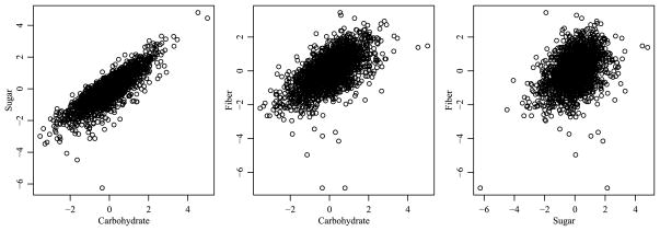
The data on the original scale are somewhat skewed and show heteroscedasticity across the demographic variables. Since different variances across groups can lead to bias in the sums of squares, making F-tests for interactions anti-conservative [Miller and Brown (1997)], stabilizing the variance is desirable. Figure 9 provides two-way scatterplots of the response variables after applying a quarter power transformation to each variable, which we found stabilized the variances across the groups better than either a log or square-root transformation. Additionally, following the quarter power transformation, we centered and scaled each response variable to have mean zero and variance one.

Fig. 9.

Two-way plots of the transformed data.

4.1. MANOVA model and parameter estimation

As presented in Table 2 of Section 1, F-tests indicate evidence for the presence of interactions in the array of population cell means. However, 12% of all age-education-ethnicity categories have sample sizes less than 5, and so we are concerned with overfitting of the OLS estimates. As an alternative, we extend the HA methodology described in Section 2 to accommodate a MANOVA model. Our MANOVA model has the same form as the ANOVA model given by equation (1), except that each effect listed there is a three-dimensional vector corresponding to the separate effects for each of the three response variables. Additionally, the error terms now have a multivariate normal distribution with zero-mean and unknown covariance matrix Σ_y.

We extend the hierarchical array prior discussed above to accommodate the p-variate MANOVA model as follows: Our prior for the m₁ × p matrix a of main effects for the first factor is vec(a) ~ N_m1p(0, I ⊗ Σ_a), where Σ_a is as before. Our prior for the m₁ × m₂ × p array (ab) of two-way interaction terms is given by $\text{vec}(ab)~N_{m_1{m}_{2}p}(0,{\mathrm{\Gamma }}_{ab}^{-1}\otimes {\mathrm{\sum }}_b\otimes {\mathrm{\sum }}_a)$. Here, Γ_ab is a p × p diagonal matrix whose terms determine the scale of the two-way interactions for each of the p response variables. If we consider only the first response, then (Γ_ab)₁₁ is exactly the γ_ab scalar described in the ANOVA setup. Similarly, our prior for the four-way array (abc) of three-way interaction terms is $\text{vec}(\mathit{abc})~N_{m_1{m}_2{m}_{3}p}(0,{\mathrm{\Gamma }}_{\mathit{abc}}^{-1}\otimes {\mathrm{\sum }}_c\otimes {\mathrm{\sum }}_b\otimes {\mathrm{\sum }}_a)$. Priors for other main effects and interaction terms are defined similarly. The hyperpriors for each diagonal entry of Γ are independent gamma distributions, chosen as in Section 2.4 so that the prior magnitude of the effects for each response is centered around the sum of squares of the effect from the OLS decomposition.

An alternative prior would be to include a covariance matrix representing similarities of effects across the three variables. This would be achieved by replacing I ⊗ Σ_a in the prior for a with Σ_p ⊗ Σ_a, ${\mathrm{\Gamma }}_{ab}^{-1}$ with ${\mathrm{\sum }}_p{\mathrm{\Gamma }}_{ab}^{-1}$ in the prior for ab, and so on. Such a covariance term might be appropriate for data in which marginal correlations between the p response variables were driven by similarities in the cell means, rather than by within-cell correlations. In such a case we would expect, for example, that if a₁, the main effects for variable 1, were positively correlated with a₂, the main effects for variable 2, then b₁ and b₂ would be positively correlated, as would c₁ and c₂, as well as any other pair of effects in the decompositions of variables 1 and 2. However, such consistency does not appear in our NHANES data: For example, considering correlations between the ANOVA decomposition parameters for sugar and carbohydrates, we observe positive correlations for the main effects of age and education and negative correlations for the interaction terms age×ethnicity and age×ethnicity×education. These observations support the choice of Σ_p = I in the prior for the analysis of these data, although estimating Σ_p might be warranted for other data sets.

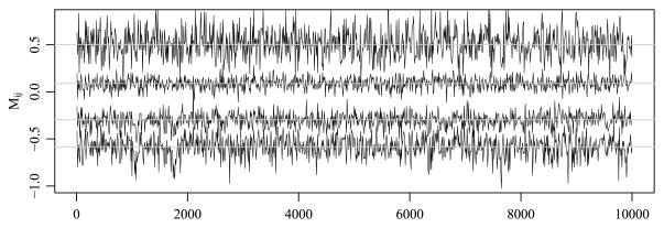
A Gibbs sampling scheme similar to the one outlined in Section 2 was iterated 200,000 times with parameter values saved every 10 scans, resulting in 20,000 simulated values of the means array M and the covariance matrices {Σ_eth, Σ_age, Σ_edu} for posterior analysis. Mixing of the Markov chain for M was good: Figure 10 shows MCMC samples of 4 out of 300 entries of M (chosen so that their trace plots were visually distinct). The autocorrelation across the saved scans was low, with the lag-10 autocorrelation for the thinned chain less than 0.14 in absolute value for each element of M (97.3% of entries have lag-10 autocorrelation less than 0.07 in absolute value) and effective sample sizes between 1929 and 13,520. The mixing for the elements of the covariance matrices Σ_eth, Σ_age, Σ_edu is not as good as that of the means array M: The maximum absolute value of lag-10 autocorrelation of the saved scans for the three rescaled covariance matrices is 0.18, 0.12 and 0.19, respectively. The effective sample sizes for the elements of the covariance matrices are at least 1684.

Fig. 10.

MCMC samples of 4 out of 300 entries of the means array M.

4.2. Posterior inference on M and Σs

We obtain a Monte Carlo approximation to M̂ = E[M|Y] by averaging over the saved scans of the Gibbs sampler. Figure 11 provides information on the shrinkage and regularization of the estimates due to the HA procedure, as compared to OLS. The first panel plots the difference between the OLS and Bayes estimates of the cell means versus cell-specific sample sizes. For small sample sizes, the Bayes estimate for a given cell is affected by the data from related cells, and can generally be quite different from the OLS estimate (the cell sample mean). For cells with large sample sizes the difference between the two estimates is generally small. The second panel of the figure plots the OLS estimates of the cell means for carbohydrate intake of black survey participants across age and education levels. Note that there appears to be a general trend of decreasing intake with increasing age and education level, although the OLS estimates themselves are not consistently ordered in this way. In contrast, these trends are much more apparent in the Bayes estimates plotted in the third panel. The HA prior allows the parameter estimates to be close to additive, while not enforcing strict additivity in this situation where we have evidence of nonadditivity via the F-tests. The smoothing provided by the HA prior is attributed to its ability to share information across levels of an effect and across interactions. When more levels are present for a particular effect, the smoothing of the HA prior closely resembles the behavior one would expect from an unbinned continuous effect. On the other hand, OLS will continue to model each cell-specific mean separately, ignoring the similarities among levels and failing to recognize the continuous nature of the effect. The third panel of the figure was also more consistently ordered than a similar analysis performed with the SB prior, suggesting that the added shrinkage due to the inverse-Wishart priors and the ability to share information across effect levels leads to more realistic behavior of the estimates.

Fig. 11.

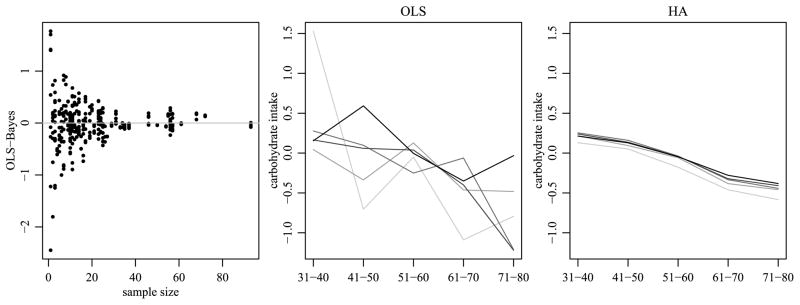
Shrinkage and regularization plots. The first panel plots the difference between the OLS and HA estimates of a cell mean against the cell-specific sample sizes. The second a third panels plot estimated cell means of carbohydrate intake for black survey participants across age and education levels, where lighter shades represent higher levels of education.

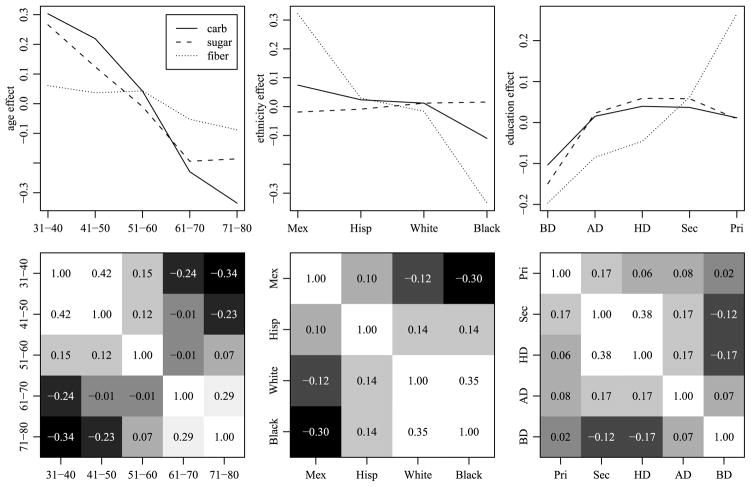
The range of cell means for the centered and scaled effects is −0.58 to 0.4 for carbohydrates, −0.38 to 0.38 for sugar and −1 to 0.51 for fiber. The average standard errors for the cell means for the three responses are 0.08, 0.09 and 0.13, respectively. When fitting the data with the SB prior (analysis not included here), the average standard errors for the cell means were substantially larger: 0.12, 0.13 and 0.15 for the three responses, respectively. The first row of Figure 12 provides the estimates of the main effects from the HA procedure. The second row of Figure 12 summarizes covariance matrices {Σ_eth, Σ_age, Σ_edu} via the posterior mean estimates of the correlation matrices $\{C_{d,ij}\}=\{{\mathrm{\sum }}_{d,ij}/\sqrt{{\mathrm{\sum }}_{d,ii}{\mathrm{\sum }}_{d,jj}}\}$ for d ∈ {eth, age, edu}. In this figure, the diagonal elements are all 1, and darker colors represent a greater departure from one. The range of the estimated correlations was −0.34 to 0.42 for age categories, −0.30 to 0.35 for ethnic groups, and −0.17 to 0.38 for educational categories. For the two ordered categorical variables, age and education, we see that closer categories are generally more positively correlated than ones that are further apart. While the ethnicity variable is not ordered, its correlation matrix informs us of which categories are more similar in terms of these response variables. The middle panel of the second row of Figure 12 confirms the order-consistent interactions we observed in Figure 2: Mexican survey participants are more similar to Hispanic participants in terms of carbohydrate intake patterns than to white or black participants.

Fig. 12.

Plots of main effects and interaction correlations for the three outcome variables (carbohydrates, sugar and fiber). The first row of plots gives HA estimates of the main effects for each factor. The second row of plots gives correlations of effects between levels of each factor, with white representing 1 and darker colors representing a greater departure from one.

For fiber intake, the top row of Figure 13 gives age by education interaction plots for each level of ethnicity, using cell mean estimates obtained from the HA procedure. Comparing these plots to the analogous plots for the OLS estimates presented in Figure 1, we see that the smoother HA estimates allow for a more interpretable description of the three-way interaction. Recall that a three-way interaction can be described as the variability of a two-way interaction across levels of a third factor. Based on the plots, the two-way age by education interactions for the Mexican and Black groups seem quite small. In contrast, the White and Other Hispanic groups appear to have interactions that can be described as heterogeneity in the education effect across levels of age. For both of these groups, this heterogeneity is ordered by age: For the Other Hispanic group, the education effects seem similar for the three youngest age groups. For the White group, the education effects seem similar for the two youngest age groups.

Fig. 13.

HA and SB interaction plots of estimated mean fiber intake by ethnicity, age and education level. HA and SB estimates are in the top and bottom rows, respectively.

This similarity in education effects for similar levels of age is more apparent in these HA estimates than in the corresponding parameter estimates from the SB procedure, presented in the second row of Figure 13, particularly for the White ethnicity. In contrast to the SB approach, the HA procedure was able to recognize the similarity of parameters corresponding to adjacent age levels and to use this information to assist with estimation. Our expectations that age effects are likely to be smooth, as well as the good performance of the HA procedure in the simulation study of the previous section, give us confidence that the HA procedure is providing more realistic and interpretable cell mean estimates than either the OLS or SB approaches.

5. Discussion

This article has presented a novel hierarchical Bayes method for parameter estimation of cross-classified data under ANOVA and MANOVA models. Unlike least-squares estimation, a Bayesian approach provides for regularized estimates of the potentially large number of parameters in a MANOVA model. Unlike the nonhierarchical Bayesian approach, the hierarchical approach provides a data-driven method of regularization, and unlike the standard hierarchical Bayes, the hierarchical array prior can identify similarities among categories and share this information across interaction effects to assist in the estimation of higher-order terms for which data information is limited. In a simulation study the HA approach was able to detect interactions when they were present, and to estimate the means array better than a full least squares or standard Bayesian approaches (in terms of mean squared error). When the true means array was completely additive, the HA prior was able to adapt to this smaller model better than the other full model estimation approaches under consideration.

An immediate extension to our approach modifies the priors on the covariance matrices to incorporate known structure. For example, in the case of observations for different time periods, an autoregressive covariance model might be desirable. In the simplest case of an AR(1) model, Berger and Yang (1994) suggest the use of a reference prior π_R(ρ) for the single parameter ρ. We also note that due to the scale nonidentifiability of the Kronecker product we can assume that the variance parameter is equal to 1. The posterior approximation follows the outline of Section 2.2: the full conditionals for the effects and the full conditionals for the covariance matrices that do not exhibit a specific structure remain the same. The only difference is in the posterior approximation procedure for the structured covariance matrix, where a posterior sample of ρ can be obtained by importance sampling. The HA procedure can easily accommodate other structured covariances as well, with the only changes to the posterior approximation steps reflecting this additional prior information for the covariance matrix.

Generalizations of the HA prior are applicable to any model whose parameters consist of vectors, matrices and arrays for which some of the index sets are shared. This includes generalized linear models with categorical factors, as well as ANCOVA models that involve interactions between continuous and categorical explanatory variables. As an example of the latter case, suppose we are interested in estimating the linear relationship between an outcome and a set of explanatory variables for every combination of three categorical factors. The regression parameters then consist of an m₁ × m₂ × m₃ × p array, where m₁, m₂, m₃ are the numbers of factor levels and p is the number of continuous regressors. The usual ANCOVA decomposition can be used to parametrize this array in terms of main effects and interactions arrays, for which a hierarchical array prior may be used.

Computer code and data for the results in Sections 3 and 4 are available in the supplementary material [Volfovsky and Hoff (2013)].

References

- Albrink MJ, Ullrich IH. Interaction of dietary sucrose and fiber on serum lipids in healthy young men fed high carbohydrate diets. Am J Clin Nutr. 1986;43:419–428. doi: 10.1093/ajcn/43.3.419. [DOI] [PubMed] [Google Scholar]
- Austin GL, Ogden LG, Hill JO. Trends in carbohydrate, fat, and protein intakes and association with energy intake in normal-weight, overweight, and obese individuals: 1971–2006. Am J Clin Nutr. 2011;93:836–843. doi: 10.3945/ajcn.110.000141. [DOI] [PubMed] [Google Scholar]
- Basiotis PP, Thomas RG, Kelsay JL, Mertz W. Sources of variation in energy intake by men and women as determined from one year’s daily dietary records. Am J Clin Nutr. 1989;50:448–453. doi: 10.1093/ajcn/50.3.448. [DOI] [PubMed] [Google Scholar]
- Beran R. ASP fits to multi-way layouts. Ann Inst Statist Math. 2005;57:201–220. [Google Scholar]
- Berger JO, Yang R-y. Noninformative priors and Bayesian testing for the AR(1) model. Econometric Theory. 1994;10:461–482. [Google Scholar]
- Chandalia M, Garg A, Lutjohann D, von Bergmann K, Grundy SM, Brinkley LJ. Beneficial effects of high dietary fiber intake in patients with type 2 diabetes mellitus. N Engl J Med. 2000;342:1392–1398. doi: 10.1056/NEJM200005113421903. [DOI] [PubMed] [Google Scholar]
- Cui Y, Hodges JS, Kong X, Carlin BP. Partitioning degrees of freedom in hierarchical and other richly parameterized models. Technometrics. 2010;52:124–136. doi: 10.1198/TECH.2009.08161. [DOI] [PMC free article] [PubMed] [Google Scholar]
- Dawid AP. Some matrix-variate distribution theory: Notational considerations and a Bayesian application. Biometrika. 1981;68:265–274. [Google Scholar]
- Friedman J, Hastie T, Tibshirani R. A note on the group lasso and a sparse group lasso. 2010. Available at arXiv:1001.0736. [Google Scholar]
- Gelman A. Analysis of variance—Why it is more important than ever. Ann Statist. 2005;33:1–53. [Google Scholar]
- Gelman A, Hill J. Data analysis using regression and multilevel hierarchical models. 2007. Unpublished manuscript. [Google Scholar]
- Genkin A, Lewis DD, Madigan D. Large-scale Bayesian logistic regression for text categorization. Technometrics. 2007;49:291–304. [Google Scholar]
- Hodges JS, Sargent DJ, Cui Y, Carlin BP. Smoothing balanced single-error-term analysis of variance. Technometrics. 2007;49:12–25. [Google Scholar]
- Hoff PD. Separable covariance arrays via the Tucker product, with applications to multivariate relational data. Bayesian Anal. 2011;6:179–196. [Google Scholar]
- Johansson G, Wikman A, Ahren AM, Hallmans G, Johansson I, et al. Underreporting of energy intake in repeated 24-hour recalls related to gender, age, weight status, day of interview, educational level, reported food intake, smoking habits and area of living. Public Health Nutrition. 2001;4:919–928. doi: 10.1079/phn2001124. [DOI] [PubMed] [Google Scholar]
- Kass RE, Wasserman L. A reference Bayesian test for nested hypotheses and its relationship to the Schwarz criterion. J Amer Statist Assoc. 1995;90:928–934. [Google Scholar]
- Kolda TG, Bader BW. Tensor decompositions and applications. SIAM Rev. 2009;51:455–500. [Google Scholar]
- Kruschke J. Doing Bayesian Data Analysis: A Tutorial Introduction with R and BUGS. Academic Press; Boston, MA: 2011. [Google Scholar]
- Miller R, Brown B. Beyond ANOVA: Basics of Applied Statistics. Chapman & Hall/CRC; New York: 1997. [Google Scholar]
- Moerman C, De Mesquita H, Runia S. Dietary sugar intake in the aetiology of biliary tract cancer. International Journal of Epidemiology. 1993;22:207–214. doi: 10.1093/ije/22.2.207. [DOI] [PubMed] [Google Scholar]
- Montonen J, Knekt P, Järvinen R, Aromaa A, Reunanen A. Whole-grain and fiber intake and the incidence of type 2 diabetes. Am J Clin Nutr. 2003;77:622–629. doi: 10.1093/ajcn/77.3.622. [DOI] [PubMed] [Google Scholar]
- Nielsen SJ, Popkin BM. Changes in beverage intake between 1977 and 2001. Am J Prev Med. 2004;27:205–210. doi: 10.1016/j.amepre.2004.05.005. [DOI] [PubMed] [Google Scholar]
- Olson C. On choosing a test statistic in multivariate analysis of variance. Psychological Bulletin. 1976;83:579. [Google Scholar]
- Park T, Casella G. The Bayesian lasso. J Amer Statist Assoc. 2008;103:681–686. [Google Scholar]
- Park D, Gelman A, Bafumi J. Public Opinion in State Politics. Stanford Univ. Press; Stanford, CA: 2006. State level opinions from national surveys: Post-stratification using multilevel logistic regression; pp. 209–228. [Google Scholar]
- Park Y, Subar AF, Hollenbeck A, Schatzkin A. Dietary fiber intake and mortality in the NIH-AARP diet and health study. Arch Intern Med. 2011;171:1061–1068. doi: 10.1001/archinternmed.2011.18. [DOI] [PMC free article] [PubMed] [Google Scholar]
- Pittau M, Zelli R, Gelman A. Economic disparities and life satisfaction in European regions. Social Indicators Research. 2010;96:339–361. [Google Scholar]
- USDA. Food and Nutrient Database for Dietary Studies 4.1. U.S. Dept. Agriculture, Agricultural Research Service, Food Surveys Research Group; Beltsville, MD: 2010. [Google Scholar]
- Verly E, Junior, Fisberg RM, Cesar CLG, Marchioni DML. Sources of variation of energy and nutrient intake among adolescents in São Paulo. Brazil Cadernos de Saúde Pública. 2010;26:2129–2137. doi: 10.1590/s0102-311x2010001100014. [DOI] [PubMed] [Google Scholar]
- Volfovsky A, Hoff P. Supplement to “Hierarchical array priors for ANOVA decompositions of cross-classified data”. 2013. [DOI] [PMC free article] [PubMed] [Google Scholar]
- Yang EJ, Chung HK, Kim WY, Kerver JM, Song WO. Carbohydrate intake is associated with diet quality and risk factors for cardiovascular disease in us adults: Nhanes iii. Journal of the American College of Nutrition. 2003;22:71–79. doi: 10.1080/07315724.2003.10719278. [DOI] [PubMed] [Google Scholar]
- Yuan M, Lin Y. Efficient empirical Bayes variable selection and estimation in linear models. J Amer Statist Assoc. 2005;100:1215–1225. [Google Scholar]
- Yuan M, Lin Y. Model selection and estimation in regression with grouped variables. J R Stat Soc Ser B Stat Methodol. 2006;68:49–67. [Google Scholar]
- Yuan M, Lin Y. Model selection and estimation in the Gaussian graphical model. Biometrika. 2007;94:19–35. [Google Scholar]
Associated Data
This section collects any data citations, data availability statements, or supplementary materials included in this article.