

Abstract
Surface-based cortical registration methods that are driven by geometrical features, such as folding, provide sub-optimal alignment of many functional areas due to variable correlation between cortical folding patterns and function. This has led to the proposal of new registration methods using features derived from functional and diffusion imaging. However, as yet there is no consensus over the best set of features for optimal alignment of brain function.
In this paper we demonstrate the utility of a new Multimodal Surface Matching (MSM) algorithm capable of driving alignment using a wide variety of descriptors of brain architecture, function and connectivity. The versatility of the framework originates from adapting the discrete Markov Random Field (MRF) registration method to surface alignment. This has the benefit of being unconstrained by choice of a similarity measure and relatively insensitive to local minima. The method offers significant flexibility in the choice of feature set, and we demonstrate the advantages of this by performing registrations using univariate descriptors of surface curvature and myelination, multivariate feature sets derived from resting fMRI, and multimodal descriptors of surface curvature and myelination. We compare the results with two state of the art surface registration methods that use geometric features: FreeSurfer and Spherical Demons. In the future, the MSM technique will allow explorations into the best combinations of features and alignment strategies for inter-subject alignment of cortical functional areas for a wide range of neuroimaging datasets.
Keywords: Surface-based cortical registration, Multimodal, Functional Alignment, Discrete Optimisation
1. Introduction
Surface registration algorithms offer advantages over volumetric approaches for alignment of the sheet-like cerebral cortex. These model the cortical sheet as a two-dimensional mesh and inflate it to a sphere, thereby simplifying the three-dimensional volumetric registration problem to a two-dimensional surface registration problem with a simpler geometry. This geometry better represents the (neurobiologically more meaningful) geodesic distances between points on the cortex.
Alignment of cortical surfaces is commonly driven using geometric features that describe measures of cortical shape (folding), such as sulcal depth or local curvature (Fischl et al., 1999a; Yeo et al., 2010). This has allowed surface-based registrations to significantly improve the alignment of cortical folds relative to volumetric approaches (e.g. Ghosh et al. (2010)). Unfortunately, cortical folding is not consistent across subjects in many brain regions, for example, the cingulate sulcus is highly variable in terms of its branches and interruptions (Van Essen, 2005). This limits folding-based surface registration methods since, in regions where the number of anatomical folds differ across individuals, there cannot be a one-to-one matching based on folding alone. In such circumstances, pointwise registration algorithms such as FreeSurfer (Fischl et al., 1999b) and Spherical Demons (Yeo et al., 2010) are forced to obtain a match by expanding or contracting the additional anatomical folds in a way that is not biologically informed, which can lead to severe local distortions.
Alternative methods have been developed that use the variability of folds (Auzias et al., 2013). However, a more fundamental limitation of morphologically driven alignment is that cortical folds do not always match the underlying cortical microarchitecture, such as cytoarchitecture and myeloarchitecture. These microscopic features are known to match brain function more closely than folding patterns alone (Amunts et al., 2007). The limitation of folding-driven alignment in this context was demonstrated by Fischl (Fischl et al., 2008), who performed FreeSurfer alignment of cytoarchitectural segmentations of postmortem brains. The study showed that while folding-driven alignment of some cortical areas, such as primary visual and motor areas was fairly accurate, other areas, such as Brodman areas 44 and 45, or area hOC5 in extrastriate visual cortex, had poor inter-subject overlap (Fischl et al., 2008; Van Essen, 2012). Given that a major goal of intersubject registration is to co-localise functional subregions across subjects, the Fischl et al. (2008) result suggests that alignment driven by folding patterns alone is insufficient for meeting this objective.
These observations have motivated the formulation of alternative approaches that aim to align brain function directly using features derived from functional MRI. In one example, Sabuncu et al. (2010) drove alignment of brain regions using correlations of functional responses to a movie-watching task. However, this restricts the approach to tasks that exhibit time-locked responses, and can only reliably align brain regions that the task activates consistently across subjects. Therefore, Conroy and colleagues (Conroy et al., 2013) improved upon this result by aligning global functional connectivity matrices. Nevertheless, both approaches require initialisation using folding based alignment, and it is our opinion that further improvements could be gained by the inclusion of information from other MRI modalities.
A multimodal feature set requires a flexible registration framework. For this purpose, we choose to work with a discrete optimisation framework (Kolmogorov, 2006; Komodakis and Tziritas, 2007; Komodakis et al., 2008; Wainwright et al., 2002). A major motivation for this choice is the flexibility it offers in the selection of similarity measures (Glocker et al., 2008; Kwon et al., 2011; Ou et al., 2011), as it is not currently clear how different features covary across subjects, nor what set of features is the most optimal for driving alignment.
Discrete optimisation for registration of volumetric MRI brain images was first proposed by Glocker et al. (2008), where it was shown to offer significant speed improvements over continuous B-spline free-form deformation approaches (Rueckert et al., 1999), whilst generating equally accurate results. Discrete approaches are also less sensitive to local minima than continuous optimisation techniques, which aids with the alignment of the complex folding patterns across subjects. However, one limitation of the discrete approach is that the choice of grid and number of labels (discrete displacement options) has a significant impact on the computational burden of the problem. Furthermore, the discretisation of the deformation places some limits on the achievable accuracy. Consequently, it has become common practice within discrete volumetric approaches (Glocker et al., 2008) to reduce the degrees of freedom by using a multi-resolution series of control point grids within a B-Spline deformation framework, similar to those used by continuous approaches (Rueckert et al., 1999; Andersson et al., 2007). As a result, the guarantees regarding discrete optimisation finding the globally optimal solution do not hold in the multi-resolution setting, although this is also the case for almost all continuous approaches.
One other limitation of the discrete optimisation approach is that including higher order regularization functions becomes very difficult (Glocker et al., 2009; Kwon et al., 2011), even though the similarity measure can be chosen very flexibly. However, we have found that the advantages of the discrete optimisation framework outweigh the disadvantages for our application. More detailed discussions of the relative merits of the discrete optimisation framework can be found in the discussion section.
In this paper we build on the discrete optimisation framework described in Glocker et al. (2008) to achieve surface registration. Crucially, our framework enables multiple sources of information (distinct features, intensities or modalities) to be used to drive registration. We adapt this framework in three ways. First, we describe how displacement of each surface vertex is represented in terms of a discrete set of possible rotations. We also propose a new regularization term, customised for the spherical surface, and based on penalising the geodesic distance between rotation matrices. In addition, we present a multivariate mutual-information similarity measure derived from entropic graphs (Neemuchwala, 2005; Staring et al., 2009), that we adapt to the discrete setting. This allows great flexibility of the framework with regards to choice of features.
The results here extend work presented in Robinson et al. (2013), in which the utility of the Multimodal Surface Matching framework for surface registration was demonstrated through use of simulation and preliminary analyses using neurobiological data. Here, we significantly expand these analyses and present results using new multivariate and multimodal MRI data. Our primary goal with this paper, and set of results, is to demonstrate that the proposed discrete optimisation framework is highly flexible and is capable of aligning cortical surfaces using a variety of different feature sets, in ways that improve functional co-localisation. To this end: Section 5.2 shows that the discrete method can perform folding-based alignment with similar accuracy and areal distortion as two state-of-the-art continuous methods (FreeSurfer (Fischl et al., 1999a) and Spherical Demons (Yeo et al., 2010)); and Section 5.3 shows how high-quality resting-state functional MRI alignment is sufficiently generalisable to also improve the alignment of task activations. In this paper, we aim to demonstrate the broad applicability and flexibility of this method but do not wish to imply that any of the parameter settings used to run the software on specific datasets are optimal. We also do not set out to systematically explore which combination of features is most suited for the best registration. These issues are the focus of current and future work, and will be reported in future publications.
Alignment of multimodal MRI data is a highly complex problem due to the often contrasting nature of the different datasets. Specifically, functional regions often traverse cortical folds and, as yet, there is no known one-to-one matching between functional and structural connectivity. We believe that optimal alignment using combinations of features will require the learning of cost function weightings, or subsets of features regionally. This is particularly complex given the lack of ground truth regarding the reliability of each feature for defining functional boundaries. For this reason much of the focus of this paper is on serial alignment of multimodal MRI features. Nevertheless, section 5.4 demonstrates the capability of the method for simultaneous multimodal alignment using a combination of folding and myelin data.
2. Discrete optimisation for registration
In this section we describe the principles of discrete optimisation for registration for a general audience. More comprehensive overviews, with technical details, can be found in Glocker et al. (2008, 2011) and Wang et al. (2013).
Registration aims to find a spatial transformation that maps one image M (moving image) to another F (fixed or reference image), in a way that aligns quantities of interest. Discrete optimisation can be applied in registration using a discrete Markov Random Field (MRF) labelling where these labels2 represent discrete displacements of each point in the moving image. That is, there are a fixed, finite number of possible displacements for each point, as opposed to the continuous optimisation approach that allows an infinite number of possible displacement vectors.
The moving image is deformed by warping a grid of points, P (Figure 1A), which can represent the native voxel grid or a lower-resolution control point grid. The optimal deformation of each vertex P is determined using a first order Markov Random Field (MRF) model:
| (1) |
where the optimal combination of label assignments (deformations) balances a data cost term cp, which measures how well the image features are aligned, with a regularization potential V, which encourages a smooth deformation by penalising neighbouring points p and q from undergoing very different displacements (as represented by the labels lp, lq respectively). Here λ is a weighting parameter and E is the set of all neighbouring point pairs (edges).
Figure 1.
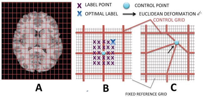
Discrete optimisation for volumetric registration: A) a lower resolution control point grid (red) is shown over the moving image. B) a set of label points (blue/purple) defines the restricted deformations possible for each control point. The spacing of the candidate label points (blue/purple) is intermediate between the lower-resolution control point grid (red) and the voxel grid of the fixed image, F (grey). C) The Euclidean deformation of a single control point to the location of its optimal label point (only one control point is moved for illustrative purposes).
Labels describe a finite set of potential displacements about each point. For example, in the volumetric framework (only used here to explain key concepts), one label might describe the translation of a point by 5 mm along the x axis whereas another might translate a point 10 mm along y. Therefore, each control point p is surrounded by a set of candidate label points, and each label point has a particular label value (e.g. the label point highlighted as optimal in Figure 1B might be called label 25, so that lp = 25 if that label is selected at point p). Control points are conditionally independent of all points given their neighbours, and are free to select different label values (Figure 1B) subject to the influence of the regularization potential V (lp, lq). In general all labels are updated (not shown in the figure) and so each point is assigned a deformation vector dlp (Figure 1C). Thus, by selecting labels for each vertex p, a non-linear deformation for the whole grid is defined.
The data cost for each control point, and each label lp, is calculated by:
| (2) |
where ρ is a function that quantifies differences between features; dlp is a Euclidean transformation defined by the control point label value lp; M (xi) is the feature (vector) at vertex i within the moving image; F(xi + T0(xi)+ dlp) is the feature (vector) from the fixed image, corresponding to the location of xi in the moving image, and with T0(xi) representing any initial transformation, such as those generated from previous iterations3, and Np is a local image patch centred at the control point. This subdivides the higher resolution image data into zones of influence for different control points using, for example, linear weighting terms (Glocker et al., 2008).
Finally, to reduce the computational burden it is common to use a multi-resolution approach (Figure 1A), as in many other registration methods (Rueckert et al., 1999; Andersson et al., 2007). This approach reduces the number of discrete labels needed at each stage, with the deformations up-sampled using B-spline interpolation between resolution steps, allowing high-resolution registrations to be achieved despite the limitation of having only discrete vectors.
3. The spherical registration framework
In this section we explain our novel adaptation of the generic discrete optimization framework (described above) to a spherical geometry. This begins by generating a series of control point grids from regular subdivisions of an icosahedron (Figure 2A); typically, subdivisions of order 2 to 5 are used (with 161, 642, 2542 or 10242 vertices), giving mean vertex distances (MV D) of 26.7mm, 13.8mm, 6.9mm or 3.5mm, for a sphere of radius 100mm. Deformations are upsampled from the control grid to the moving mesh M with Thin Plate Spline interpolation (Bookstein, 1989), using Radial Basis Functions to create a smooth spatial mapping for every point in M given the displacement of surrounding control points. This provides an additional level of regularization.
Figure 2.
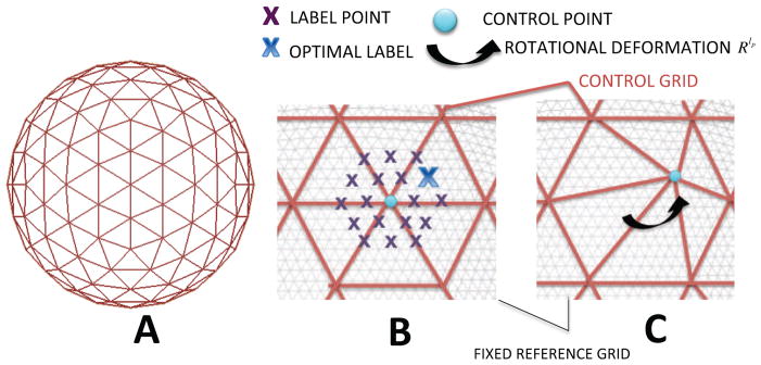
Discrete optimisation for spherical registration: A) The control point grid (red) is formed from a regular subdivision of an icosahedron. B) Regularly spaced label points are placed around the control point using a higher resolution icosahedron to define a sampling grid for the candidate label points (purple/blue points); this grid has lower resolution than the fixed (and moving) mesh (grey); C) Deformation of a control point to its optimal label point (only one control point is moved for illustrative purposes), using rotations about the centre of the sphere (not Euclidean vectors).
Human cortical surface meshes, as initially generated using FreeSurfer, contain on the order of 140,000 vertices per hemisphere, with vertex spacings of approximately 1mm. The MSM framework downsamples the high-resolution surfaces MH and FH onto regular icosahedral meshes, M and F. The degree of downsampling varies across control point grid resolutions. In general, image data is maintained at least two icospheric subdivisions higher than control point grids, and image patches (Np in Equation 4) are defined as circles whose radii are determined by the maximum separation between the current control point p and its neighbouring control points. We find, subdividing to a regular mesh of 10,242 (3.5mm spacing, subdivision 5) or 40,962 (1.7mm, subdivision 6) vertices provides useful speed-ups of the calculations (Equation 4) without appreciably degrading the accuracy of the alignment.
3.1. Definition of the label set
The key conceptual difference between the application of discrete optimisation in spherical (as opposed to volumetric) registration comes from the definition of the label set.
In the volumetric setting it is very common to have the same label represent the same deformation for each of the control points within a given iteration. Hence if two neighbouring control points p and q were deformed by labels lp and lq, and lp = lq =‘16’, then both points would deform in exactly the same way for that iteration. However, with spherical geometry such consistent, global deformations are difficult to define.
For example, an equivalent Euclidean deformation at each point on the sphere would result in control points deforming to a location no longer on the spherical surface. If instead an equivalent rotational deformation was used, then points at the poles would never deform as much as points on the equator of the sphere. Therefore, we define labels using a set of evenly spaced points surrounding each control point (Figure 2B). To obtain evenly spaced samples on the surface we use an icosahedral subdivision that is 2 orders of resolution higher than the control point grid. Each point is represented by a label value (e.g. lp = ‘16’ for the optimal label shown in the Figure 2C).
To ensure that a similar set (with fixed number) of deformations exist for all p ∈ P, a single set of sampling grid vertices, surrounding the point p, is used as a template for the label point set. This template set is then copied and moved so that each control point has an equivalent set, with the central sampling point aligned to each control point. This solves the problem that a regular icosahedron has varying numbers (5 or 6) of faces adjacent to each vertex. Using the same sampling grid ensures the same numbers of labels for each control point (which is a minimal requirement for solving the MRF problem using optimisation methods such as the Fast-Primal Dual (Fast-PD) method (Komodakis and Tziritas, 2007; Komodakis et al., 2008)), but unlike volumetric methods does not enforce equivalence between the deformations prescribed for each label (especially at the poles – see Appendix A).
Deformations, Rlp, are defined in terms of rotations between the control point vertex and each label point, and are internally represented by rotation matrices. These matrices are calculated using the Rodrigues rotation formula:
| (3) |
where the axis k = xp×xlp/|xp×xlp| and angle θ = arcsin(|xp×xlp|/|xp||xlp|) of rotation are defined from the positions of the control point, xp and label point, xlp, with respect to the centre of the spherical grid; I is the identity matrix and [k]× is the skew-symmetric matrix:
Under this formulation the data cost term is now calculated as:
| (4) |
where RT0represents an initial transformation, as denoted by T0(xi) in equation 2.
The maximum sampling distance, and thus biggest possible control point deformation in each iteration, is set to 0.4 times the mean vertex spacing of the control points. This discourages disruption of topological relationships that would occur if the mesh were allowed to fold over onto itself. Such a constraint has been shown to enforce diffeomorphisms within the framework of regular volumetric spline-based interpolation (Rueckert et al., 2006), although for irregularly spaced control points on a spherical surface this is not yet proven. After each iteration the deformation is projected to the moving mesh M via Thin Plate Spline (TPS) interpolation, and control points are reset to their initial positions. As this interpolation and projection is performed in a piecewise fashion (where subsets of vertices in the higher resolution mesh are each transformed by a separate TPS) an unfolding step, to prevent non-diffeomorphic behaviour, is implemented here. This procedure replicates that performed in Spherical Demons (source code publicly available4). In this way deformations are composed and stored at the level of the moving mesh.
The constraint on the deformation space means that optimal alignment is not usually reached within one iteration. Therefore, the algorithm iterates over several cycles at each resolution, however, unless the label set is changed between cycles no further improvement of the registration is achieved (Glocker et al., 2008). So, the label set alternates between using the vertices and the barycentres of the sampling grid as label points (which is different from the approach in (Glocker et al., 2008)). In general, there are between 10 and 30 labels per control point, depending on control grid resolution and choice of label set. Spacing between labels at the highest label grid resolution (163,842 vertices) is approximately 0.5mm. This is given by the mean distance between each barycentre and neighbouring vertex.
3.2. Regularization
Regularization is implemented using pairwise edge potentials (between neighbouring points). Volumetric methods typically penalise Euclidean distances between Cartesian deformation vectors applied to neighbouring control points p and q, using potentials of the form: V (lp, lq) = |dlp −dlq|. However, our spherical method represents deformations as rotations and so it penalises differences between the proposed rotation matrices based on geodesic distances on the sphere:
| (5) |
where ||.||F represents the Frobenius norm. This is proportional to the angle θpq between the start and end points of the two consecutive rotations (Huynh, 2009; Moakher, 2002) (since the rotation is related to its axis angle representation through an exponential map, logR = ([k]×θ), and the Frobenius norm of the skew symmetric matrix is , where |k| is the Euclidean norm of k).
To understand this more intuitively, consider two adjacent control points p and q that select the same labels, i.e., lp=lq. The position of the sampling points (xp, xlp) relative to each control point will therefore be the same or very close, and thus the rotational matrices, Rlp and Rlq, will be quite similar (see Appendix A), the combined rotation (forward and back), (Rlp)TRlq will be close to the identity, and the geodesic distance near zero. On the other hand, if the two control points choose different labels (lp ≠ lq), the rotations involved will be less similar, and the combined rotation (forward and back) will not be so close to the identity, with the penalty term proportional to the squared angular distance of the combined rotation (Rlp)TRlq.
This basic formulation only allows regularization of a single iteration of the optimisation framework, since the control point grid is reset after every iteration, and so it effectively excludes the contribution of the deformations from previous iterations. Therefore, in order to additionally penalise incremental changes in the configurations of neighbourhoods over successive iterations, it is necessary to approximate the full deformation of each control point from the deformation of the moving mesh, M.
To obtain this approximation, the initial position of M relative to the control point is used to identify a small set of vertices in M that surround p. The mean position of these vertices x̄pm at a later iteration is then used to define the end point of a rotation Rp starting at xp and ending at x̄pm. Rp can then be defined using equation 3, with k = xp × x̄pm/|xp × x̄pm| and θ = arcsin(|xp × x̄pm|/|xp||x̄pm|).
The full deformation for each control point p is now defined as the combination of this estimated rotation Rp, followed by the proposed deformation for this iteration Rlp, and thus the full regularization penalty term is estimated as:
| (6) |
This combined distance is non metric as the penalty need not be same for points assigned the same label: V (lp, lq) ≠ 0 if lp = lq. It is therefore necessary to select a discrete optimisation method (such as Fast-PD) that can be applied with non-metric regularization penalties.
3.3. Optimisation
Optimisation of the cost function can take many forms (see overview in (Sotiras et al., 2013)) including combinatorial (Boykov et al., 2001; Komodakis and Tziritas, 2007; Komodakis et al., 2008) or message passing (Felzenszwalb and Huttenlocher, 2004; Kolmogorov, 2006; Shekhovtsov et al., 2008; Wainwright et al., 2002; Veksler, 2005) solutions. All methods for MRF labelling have the advantage that optimisation is independent of the choice of the form of the function cp(lp). In addition, these methods avoid calculation of first or second derivatives of the cost function, and they are less sensitive to local minima, since, provided the search range of the label space is large enough, these local minima can be overstepped (Glocker et al., 2011).
In our MSM framework, optimisation is performed using the Fast-Primal Dual (Fast-PD) method of Komodakis (Komodakis and Tziritas, 2007; Komodakis et al., 2008). Fast-PD formulates the MRF as a linear program and uses an efficient, adapted max-flow algorithm to solve it. The main advantages of Fast-PD over similar combinatorial algorithms are that it is much faster and it can be used with MRFs that have non-metric regularization potentials, as required here.
3.4. Multi-modal and Multi-variate Similarity Functions
The flexibility of the discrete framework is such that a wide range of similarity functions can be used for the cp in equation 4. To this end, we have implemented normalised cross correlation (CC), normalised sum of square differences (NSSD) and normalised mutual information (NMI) in our MSM framework. To better equip the method for alignment of multimodal MRI data, we also incorporated a more general multivariate similarity measure known as α-Mutual Information (α-MI) (Neemuchwala, 2005; Staring et al., 2009). This avoids costly estimations of high dimensional histograms for comparing feature vectors by instead comparing lengths of entropic graphs.
Graphs are used in this method as a way to calculate feature similarities. The form of graph used for this is a similarity graph G(P, Nk), where the nodes of the graph P represent the vertices of the fixed and moving meshes, and edges connect each node p ∈ P to the k nodes that have the most similar feature vectors e.g. min|zp − zk| for the Euclidean distance between feature vectors zp and zk ∈ Z.
Entropic graphs have path lengths Lγ(Z) (length functionals) that are quasi additive; e.g. minimum spanning tree (MST) or k-nearest neighbour (kNN) graph (Hero et al., 2002; Neemuchwala, 2005). The path length of the kNN graph is calculated by summing the edge weights e(.) of all edges in the neighbourhood Nk,p of each node p, for all nodes:
| (7) |
Edge weights are calculated from the Euclidean distances between feature vectors zp and zk (ek,p = zp − zk) and γ is a user defined scaling exponent.
Similar to the use of path length in brain network theory (Sporns, 2006), short length functionals are indicative of graphs with more ordered structure and thus lower entropy. As such a direct relationship can be drawn to information theoretic measures of α or Rényi entropy (Hero and Michel, 1999). This allows an approximation for graph-based mutual information to be derived as (Neemuchwala, 2005):
| (8) |
where, Zf, Zm, and Zfm represent the set of feature vectors for each kNN graph, D is the number of features, γ = D(1−α), and α (0 < α < 1) relates to α-entropy, with higher values giving more weight to high probability events.
The quantities and represent kNN components of length functionals for each of the fixed, moving and joint distributions respectively (Staring et al., 2009):
| (9) |
| (10) |
| (11) |
where and are the separate neighbourhood clusters for each graph, and vector is a concatenation of the feature vectors and .
This measure essentially estimates the divergence between the joint feature distribution p(zfm) and the marginals p(zf) and p(zm). Mutual information is maximised when clusters representing similar structures in the fixed and moving datasets are made to align. In such instances the nearest neighbours of the joint distribution should coincide with those in the marginals, and all distances will be minimised.
4. Implementation details
In summary, the minimal requirement for running the MSM algorithm is a pair of cortical surface meshes, inflated to the sphere (we have used FreeSurfer extracted surfaces but this is not a restriction), and a set of features for the surface. Features in this context can mean any combination of surface features for example: 1) cortical folding alone; 2) multivariate features of structural or functional connectivity targets (and their weights); 3) multimodal combinations of surface folding and myelination; 4) all of the above.
Registration runs over several control point grid resolution levels (CPres), where at each level the data associated with the fixed and moving meshes are typically downsampled (to a resolution DPres) using Gaussian interpolation (smoothing kernel σ). Labels are defined through a sampling scheme, which uses a regular icosahedral grid, several (usually 2) orders of resolution higher than the control grid to define end points of local deformations. The sampling grid resolution (SPres), and thus deformation scale, may also update at each level. The parameters: CPres, DPres, SPres, σ, as well as the choice of similarity function ρ (equation 4) can be tuned by the user and input to the algorithm in the form of a configuration file (settings used to generate results in this paper can be found in the supplementary material). The code runs on Linux and MacOS, and the software will be made available in a forthcoming release of the FMRIB Software Library (Jenkinson et al., 2012).
5. Experimental methods
The aim of the experiments presented here is to demonstrate the flexibility of the MSM method and its wide range of applications. Although some comparisons with existing software are performed for structural alignment, it is not our intention to focus on these comparisons. Instead we want to highlight how this method creates new opportunities, by using new combinations of data to drive registration, and demonstrating initially promising results in these cases. We believe that this is a step towards finding biologically-meaningful alignments that relate structural and functional brain architecture. Therefore, these experiments should be considered as merely a sample from a broad set of potential applications.
5.1. Data Collection
We have validated MSM using data from the WU-Minn Human Connectome Project (HCP) (http://humanconnectome.org). The HCP is collecting and sharing neuroimaging data from a large group of healthy adults (ages 22 – 35, target number of 1,200 participants). HCP datasets are collected from participants during a 2 day visit that includes extensive behavioural testing plus four MRI imaging modalities (structural, diffusion, resting-state fMRI, and task-fMRI) (Van Essen et al., 2013). The data used in the following analyses were derived from structural and functional scans (resting state and task) collected from 196 subjects. A subset of 25 subjects was used for analysing univariate and multimodal alignments.
Scanning protocols for the structural image scans include 0.7mm isotropic acquisitions collected on a Siemens 3T Skyra platform, using a 32-channel head coil and MPRAGE (T1w) and SPACE (T2w) sequences (Glasser et al., 2013). Functional images were acquired using multiband (factor 8) 2mm Gradient-Echo EPI sequences (Moeller et al., 2010). Four resting state fMRI (rfMRI) scans were acquired (two successive 15 minutes scans in each of two sessions) (Smith et al., 2013a). Seven task-fMRI (tfMRI) experiments were conducted, including: working memory, gambling, motor, language, social cognition, relational, and emotional tasks; tfMRI scans were acquired after the rfMRI scans in each of two hour-long sessions on separate days (Barch et al., 2013). Additional details regarding specific acquisition parameters and task protocols are available in Barch et al. (2013) and Smith et al. (2013a), as well as on the HCP website5.
Generation of surface meshes and associated shape features were carried out using HCP Structural Pipelines (Glasser et al., 2013). This includes refinements to the standard FreeSurfer protocol (Fischl, 2012) in order to accurately extract cortical surfaces using both T1w and T2w images. Each hemisphere’s surface was mapped to a sphere by projecting points along the average convexity or concavity of a region. Metric distortions are minimised (but not eliminated) during inflation by seeking to maintain the geodesic distances between neighbouring points along the anatomical surface (Fischl et al., 1999a). For this reason we do not enforce further distortion correction terms within the registration framework.
For cortical shape features, we used FreeSurfer’s ‘sulc’ measure (‘average convexity’, which is similar but not identical to measures of sulcal depth) and mean curvature (which provides a finer-grained indicator of gyral and sulcal folds). We also used cortical myelin maps, based on the ratio of T1w to T2w images as an architectonic marker that correlates with many functionally distinct areas in individual subjects (Glasser and Van Essen, 2011).
In addition to the subjects’ native meshes, a standard 32K reference mesh (FS LR 32k) was used for analysis of fMRI data (Glasser et al., 2013). The 32K mesh is a low (2mm) resolution reference surface, with equal vertex spacing on the sphere, that has left and right hemisphere correspondence (Van Essen et al., 2012). Alignment of the data to this reference surface was initially performed using FreeSurfer registration to the FreeSurfer population average target (fsaverage), followed by a standard transformation of fsaverage to the target surface, that accounts for the assignment of left-right correspondences (Van Essen et al., 2012). After careful application of fMRI distortion correction, and following the HCP Functional Pipelines (Glasser et al., 2013), fMRI data was projected from the volume to the 32K surface using ribbon-constrained volume to surface mapping. This was followed by resampling of the subject’s native mesh to the reference surface using adaptive barycentric interpolation.
Functional data was smoothed on the surface using a 2mm FWHM geodesic Gaussian smoothing kernel, and patterns of activation (responses to each of the tasks) were modelled using FSL’s FEAT (Jenkinson et al., 2012; Smith et al., 2004; Woolrich et al., 2009), separately for each of the 86 different contrasts, over 7 different experiments. Resting-state fMRI features were derived by first performing Independent Component Analysis (ICA) (Smith et al., 2013a). This reduced the order of the connectivity features from 91,282 (the standard grayordinates space, Glasser et al. (2013)) to 26 ICA components. ICA was run on the group-wise concatenated time series data following dimensionality reduction using a specially adapted principle component analysis known as MIGP (Melodic’s Incremental Group-PCA, Smith et al. (2013a)). Following this, a set of matched components (spatial maps and associated timecourses) were generated across subjects through the process of Dual Regression (Beckmann and Smith, 2004); first regressing group maps onto subjects’ timeseries data to produce a set of component timecourses, and then regressing these to obtain a set of 26 corresponding spatial maps for each individual. Dual regression was performed for the full Q3 release of 196 subjects available from the HCP. The analysis here forms a subset of work scheduled to be released in a future publication.
5.2. Univariate alignment
We first evaluated the performance of the MSM algorithm relative to FreeSurfer (Fischl et al., 1999a) and Spherical Demons (Yeo et al., 2010) using three univariate feature sets: sulc (average convexity), curvature and cortical myelin maps. In each case, registration is driven to population averages, where the sulc and curvature population averages are taken directly from FreeSurfer, and the myelin average is generated through several rounds of MSM alignment of myelin data, where the initial template is formed by averaging myelin data following alignment of sulc features, and then the template is iteratively refined by several rounds of myelin driven MSM.
We run two levels of regularization for MSM: one “high” and one “low”, being roughly one order of magnitude different in the λ values used in equation 1 (see supplementary material for exact parameter settings). Two levels of regularization were chosen because we found in our preliminary investigations that although lower levels of regularization performed better for aligning geometric features, higher levels of regularization appeared to perform better at aligning functional data, whilst also producing smaller deformations that subjectively appeared more biologically plausible. Therefore, although we explicitly do not aim to find the “optimal” parameters in this initial work, we will use these two regularization levels in most of the experiments, to demonstrate the important effects of regularization. For clarity, we refer to each registration based on the algorithm (FS, SD, MSMhi, or MSMlo) and the modality used (sulc, curv, or myelin), combined appropriately (FS-sulc; SD-curv; MSMhi-sulc, MSMlo-sulc, etc). Here univariate registration refers to registration run with univariate features.
FreeSurfer aligns surfaces by calculating a dense displacement field over all vertices on the high resolution surface mesh (140,000 vertices) from the correlations of source and target feature sets. The dense displacement field and gradient descent optimisation strategy contribute to FreeSurfer being a relatively slow algorithm (in the order of hours).
The Spherical Demons method computes a fast diffeomorphic solution to the registration problem. It is more flexible with regards to choice of features, and uses the Gauss-Newton method for fast optimisation. This requires SSD (sum of squared differences) similarity estimates to be used, which assume the feature distributions differ in intensity only by Gaussian noise. In our experiments the standard Spherical Demons software was run in Matlab using non-default parameters that were optimised for these datasets. Specifically the algorithm is modified to relax regularization by reducing the number of smoothing iterations in the second step of the demons algorithm, whilst simultaneously increasing the step size used in the optimisation. In addition, the number of iterations of the algorithm was increased. Further details can be found in the supplementary material. The run-time of the algorithm was less than 4 minutes.
In this comparison between the different registration methods the first registration (for each method) was always driven from each subject’s native surface to the Conte69 population average (Van Essen et al., 2012) template using ‘sulc’ features (average convexity). This approach provides the closest correlate to FreeSurfer registration (Fischl et al., 1999a), as FreeSurfer allows only for sulc-driven registration, on the basis that these features display the lowest population variance among available geometric features. For Spherical Demons and MSM, registration was also evaluated using curvature and (separately) myelin features to their respective atlases, using the method-specific sulc alignment as initialisation. That is, Spherical Demons is first run on the sulc-data and then this result is used to initialise Spherical Demons when it is driven by the curvature data. When driven by myelin data the initialisation is still based on the sulc result, and does not use the curvature result. The same strategy is used for MSM, but the regularization is only varied for the sulc-driven initialisation, so that MSMhi and MSMlo only differ in the regularization used in the sulc-driven stage. The curvature stage uses the same regularization setting for both MSMhi and MSMlo, and only the initialisation is different. This is also true for the myelin stage, which only differs in the sulc-driven initialisation. See the supplementary material for full information about the parameter settings used in the different stages. In each instance MSM was run over three resolution levels (four for the myelin data) with five iterations per level and cross correlation as a similarity measure.
5.3. Resting State fMRI driven alignment
The resting state alignment was initialized using MSM-sulc (with high regularization to reduce distortions in the initial alignment), followed by MSM-myelin to align regions of cortex such as MT+ using the myelin contrast. Resting-state-driven registration then proceeds from the MSM-myelin initialization, and the final result is denoted MSM-RSN.
Feature vectors for rfMRI alignment were formed by concatenation of each subject’s 26 component ICA decomposition. The group ICA spatial maps were used as target. A limitation of the group ICA approach is that dual regressed individual subject spatial maps depend on the quality of the alignment of the data prior to ICA, and so three iterations of the registration were run in which dual regression (but not group ICA) was repeated after each step to improve the convergence.
The aim of this experiment was to evaluate the benefit of using functional connectivity features to drive the registration and see if it improves the alignment for other data sets. Therefore, the resulting transformations were used to project task activation maps into common alignment. Improvements were assessed through comparing the group mean activation maps (obtained using mixed effects FLAME (Woolrich et al., 2009)) both qualitatively and quantitatively, via cluster mass. This was done for each contrast within the set of 7 task experiments; a total of 86 contrasts. For comparison the following registration methods were also used to project the task data: FreeSurfer, MSMlo-sulc, MSMhi-sulc, and MSM-myelin. Including these methods allows the benefits of driving the registration using RSN data to be clearly separated from what is possible from sulc-driven alignment or myelin-driven alignment.
Cluster mass is calculated by the following formula: , where xi is a vertex coordinate, z(xi) is the statistical value at this coordinate, A(xi) is the area associated with this vertex (calculated from a share of the area of each mesh triangle connected to it in the mid-thickness surface), and S is the set of vertices where |z(xi)| > 10. This set of vertices above threshold is determined separately for each statistical image. The cluster mass measure reflects both the size of the super-threshold clusters and the magnitude of the statistical values within them.
For these results, in order to produce the same number of interpolations as the MSM registrations, the FreeSurfer results were “dedrifted” relative to MSM-sulc. This means that the difference in registration between FreeSurfer and MSM-sulc was calculated for each subject, and these differences (represented as deformed spherical surfaces) were averaged on a common mesh to find the average difference between FreeSurfer and MSM-sulc across the 196 subjects. The FreeSurfer aligned task fMRI data were resampled to remove this group average difference in registration (drift). This resulted in the same number of resamplings for FreeSurfer as for MSM-sulc, MSM-myelin, and MSM-RSN.
5.4. Alignment using curvature and myelin
Alignment of multimodal MRI data (i.e., simultaneous alignment of combinations of values from different MRI modalities) offers significant advantages: firstly in terms of increased speed for registration, since features are aligned in a single run as opposed to a series of sequential alignments; and secondly in terms of increased flexibility with regards to the relative weightings of features, as this allows downweighting of features in regions where they are known to be unreliable or inconsistent across subjects.
The procedure for alignment of multimodal MRI data was explored through simultaneous alignment of sulc, curv and myelin features, combined within a three-dimension feature vector. Registration was driven to a group average using α-mutual information as the similarity measure, with α set to 0.5, as this has been shown to be an optimal value for calculating the divergence of two probability distributions that are known to be very similar (Hero et al., 2002). Results were compared to registrations obtained from univariate registrations of curvature and myelin (A in Figure 6), where in each case the registrations were initialised by affine alignment of the sulc data, and registrations were driven using cross correlation as a similarity measure. Multimodal MRI registration was run using a variety of cost function weightings, labelled as for Figure 6 as: B) none; C) upweighting of cortical folds though scaling of sulc and curv features; D) upweighting of myelin features; E) use of a regionally varying costfunction weighting which scaled the contribution of the myelin relative to the folds only in areas where the myelin was known to have strong features. This was obtained by thresholding the group average myelin map, and is shown as a binary mask in the top row of result E in Figure 6 and overlaid on the group template in the second row. In each instance upweighting refers to applying a factor of 10 to the contribution from the upweighted feature, as this was found to generate a good contrast between results. All features were variance normalised prior to the application of costfunction weightings. Further details of the parameter settings can be found in the supplementary material.
Figure 6.

Multimodal alignment of sulc, curv and myelin features for a variety of costfunction weightings. Results are compared through contrasting the sharpness of the intersubject averages of the curvature and myelin features, specifically referencing the alignment of curvature in the frontal and temporal lobes (light blue arrow and white loop/arrow respectively), and myelin in the IPS (pink circle) and frontal eye fields (yellow arrow). A) presents the results obtained following univariate alignment of the curvature and myelin features individually, and is shown as a reference. Four different combinations of costfunction weightings were examined: B) no weighting; C) upweighting of the geometric features (i.e., sulc and curv) relative to myelin throughout the whole brain; D) upweighting of myelin features relative to the geometric features throughout the brain; E) upweighting of myelin features regionally according to a binary mask generated by thresholding the group myelin map (top row).
6. Results
Our overall objective was to demonstrate the robustness and flexibility of the MSM algorithm using a number of modalities individually and in various combinations. In addition, we wish to highlight the potential advantages of driving registrations using other information, such as resting-state fMRI. Complete optimization of the MSM parameters for any given modality, or combination of modalities, was not our primary objective, and we anticipate there is room for further improvement (see Discussion).
6.1. Univariate alignment
The performance of the different methods: FreeSurfer, Spherical Demons and MSM, were compared in terms of inter-subject averages and variances, areal distortion and run time of the algorithm. The average run time of the MSM algorithm was 4 minutes, which is comparable to Spherical Demons, and significantly faster than FreeSurfer, which takes several hours per subject on the platforms we used. In addition, MSM was run with both low and high regularization settings with the sulc-data, and this was used to initialise the curvature-driven and myelin-driven registrations. See the supplementary material for full details about the regularization settings.
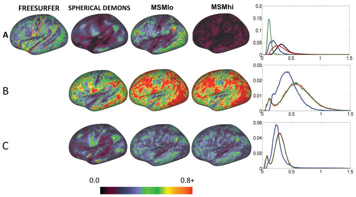
Figure 3 and Table 1 show the results of univariate alignment, compared in terms of inter-subject averages (Figure 3 rows 1,3,5) and variances (rows 2,4,6) for the left hemisphere. Figure 3A represents sulc alignments and is comparable for three methods (FreeSurfer, Spherical Demons and MSMlo), insofar as each method achieves a close match to the group average target and shows little difference in the variance maps for the algorithm parameters selected. However, MSMhi shows a clearly higher residual variance indicating that the sulcal maps are less well aligned when using high regularization. By contrast, Figure 3B displays the results of curvature alignment; in this instance FreeSurfer results were driven by sulc only (as enforced by the algorithm) and these transformations were applied to the curvature data. Spherical Demons and both MSM results were initialised by their respective sulc-driven alignments (from rows A), followed by a stage that was driven by curvature data. The regularization for the curvature-driven stage was the same for both MSM methods, with different regularizations only used in the initialisation. All three algorithms (SD, MSMlo and MSMhi) demonstrate reduced variance relative to the FreeSurfer result, with Spherical Demons having the least variance by a small margin. In both cases MSM generates a sharper and more detailed cross-subject average, possibly indicative of the high cross-subject variability in the more detailed and finer folds. Interestingly, the average and variance maps for MSMlo and MSMhi are very similar, indicating that the quality of the alignment in this case is not heavily dependent on the initialisation (difference images for these results, showing the small changes, can be found in the supplementary material). Results for myelin (Figure 3C) for the FreeSurfer method simply use the sulc-driven alignments and apply these transformations to the myelin data. The myelin-driven alignments for the other methods are only initialised by their respective sulc-driven alignments, and are completely independent of the curvature-driven alignments described previously. Regularization of the two MSM methods was the same for the myelin-driven stage. These results again show that both MSM methods are very similar, and therefore are not very dependent on the initialisation, while showing sharper delineation of features in the average maps, such as the frontal eye fields (FEF, yellow arrows) and in the area of the intra-parietal sulcus (IPS, white arrow).
Figure 3.

Results of univariate feature alignment using 25 subjects. The algorithms used are: FreeSurfer, Spherical Demons, MSM with low regularization (MSMlo) and MSM with high regularization (MSMhi). Panel A) show results of sulc-driven alignments: cross subject averages (first row) and variances (second row) across subjects. Panel B) shows curvature alignments. Panel C) shows myelin alignments. See text (section 5.2) for details of how the methods are run and initialised. Note that the cross-subject myelin average shows more structure at the positions of the frontal eye fields (yellow arrow) and intra-parietal sulcus (white arrow) for the MSM results.
Table 1.
Numeric summary of the inter-subject variance results shown in Figure 3. Mean variance for each for the three features: sulc, curv, myelin; registered using: FreeSurfer, Spherical Demons and MSM (with high and low regularization), are summarised for the left hemisphere only. In this ± stands for standard deviation (across space).
| FREESURFER | SPHERICAL DEMONS | MSMlo | MSMhi | |
|---|---|---|---|---|
| SULC | 0.207±0.108 | 0.236 ±0.097 | 0.232±0.103 | 0.278 ± 0.131 |
| CURV | 0.106±0.051 | 0.078±0.042 | 0.086±0.045 | 0.086±0.045 |
| MYELIN | 0.062±0.036 | 0.055±0.030 | 0.056±0.031 | 0.056±0.031 |
MSM and Spherical Demons tend to generate smoother distortion fields than FreeSurfer, as shown from sulc-based alignment of subjects to the Conte69 population average convexity template (Figure 4A). For each subject an areal distortion value for each vertex is calculated by averaging the distortion for all triangles adjacent to the vertex p as: , where AOi is the area of triangle i in the original mesh and ADi is the area of the corresponding triangle in the distorted mesh and Ntp is the number of triangles adjacent to vertex p. Each areal distortion map is transformed to an average template and the absolute values of distortion are averaged across subjects. Much of the difference is related to the multiresolution approach used by MSM and Spherical Demons. By contrast, FreeSurfer estimates a dense displacement field for all vertices only in the high resolution mesh where regularization is only imposed from neighbouring vertices. This analysis does not reveal which of these deformations is biologically more correct, since it did not include an independent estimate of ground truth, and the mean and variance maps are quite similar. We suspect that smoother deformations are likely to be closer to the biological truth, but this remains to be tested rigorously. Both MSM and Spherical Demons are more tuneable than FreeSurfer, providing control of the regularization weighting, and so the level of smoothness can be controlled by the user.
Figure 4.
Areal distortions from univariate alignment, across the four methods shown in figure 3: FreeSurfer, Spherical Demons, MSMlo, and MSMhi. Rows A to C correspond to panels A to C in the previous figure: registrations driven by Sulc, Curvature or Myelin. Areal distortion maps are averages across subjects, after being transformed to the population average target, and the absolute values of log2 of the area ratio is used (see text). FreeSurfer generates maps with localised distortion, particularly along gyral crowns, whereas MSMhi and Spherical Demons generate a much smoother pattern of mean distortions for Sulc- and Myelin-driven alignments. Note that MSMlo and MSMhi have substantially different distortions when driven by Sulc data, but very similar distortions for Curvature-driven or Myelin-driven cases, indicating that the differences in initialisation have little effect in these cases. Histograms (rightmost column) show all methods in each row, colour-coded as: black (FreeSurfer), blue (Spherical Demons), red (MSMlo), and green (MSMhi).
It can also be seen in these results that even though the sulc-driven results from the two MSM settings are very different in the amount of areal distortion, the effect of this as an initialisation on subsequent stages (curvature or myelin) is minimal.
6.2. Resting State fMRI driven alignment
Figure 5 shows the results of using resting-state-driven registrations to bring task fMRI data into alignment. The MSM-RSN results are compared to FreeSurfer (with drift relative to MSM-sulc removed), MSM-sulc (low regularization), MSM-sulc (high regularization), and MSM-myelin (initialised by MSM-sulc with the high regularization). In this instance, cluster mass values were calculated for data with |z| > 10, across 86 contrasts (drawn from the set of 7 independent task fMRI experiments).
Figure 5.

Task fMRI alignment driven by RSN features. The maps show group activation results from 196 subjects, thresholded at |z| > 10 for the Gambling task: reward contrast. Results are shown using a range of registration methods: FS (FreeSurfer), SulcLo (MSM-sulc with low regularization), SulcHi (MSM-sulc with high regularization), Myelin (MSM-myelin) and RSN (MSM-RSN). In the bottom left the boxplots show percentage improvement in cluster mass, across 86 task contrasts, using a threshold of |z| > 10. Median values are: 0.8%, 4.0%, 6.9% and 21.5% for SulcLo, SulcHi, Myelin and RSN respectively (and for comparison, the values for the gambling reward contrast are −0.3%, 3.0%, 5.7% and 20.5% respectively). The equivalent unthresholded maps can be found in the supplementary material.
The results show strong increases in the cluster mass index for almost all task contrasts, except when using the MSMlo-sulc method. Relative to FreeSurfer, the results from MSMlo-sulc are extremely similar on average (median change of 0.8%), as to be expected given their similar performance at aligning sulc data. The MSMhi-sulc and MSM-myelin methods show modest improvements in cluster mass (median changes of 4.0% and 6.9% respectively). Interestingly, MSMhi-sulc performs better than MSMlo-sulc, suggesting that minimizing variance of sulcal features does not yield better functional alignment, and that the lower distortions of MSMhi-sulc may be better for initialisation purposes. The biggest improvement is shown by MSM-RSN (median increase of 21.5% – see caption of Figure 5), which can clearly be attributed to the use of the resting-state data, especially since MSM-myelin is used to initialise MSM-RSN and therefore all the differences must be due to the final RSN stage.
In addition to the quantitative evaluations on the thresholded task activations, the results produced by MSM-RSN visually appear to have sharper features, suggesting that improved alignment reduces the blurring normally inherent in group averages. This can be seen in the thresholded results shown in Figure 5 as well as in the unthresholded results, shown in the supplementary material. Because the resting state features provide comprehensive coverage of the brain, they provide a robust and general functional alignment for the task data.
6.3. Multi-modal alignment of curvature and myelin
The quality of the multimodal alignments for different cost function weightings is compared by observing the sharpness of the inter-subject averages of curv and myelin features, as compared to the result obtained by univariate alignment of each feature individually. The strongest contrasts are seen for curvature features highlighted in the frontal (light blue arrow) and temporal lobes (white circles/arrows) and for myelin in the frontal eye fields (yellow arrow) and IPS (pink circle), as shown in Figure 6.
As mentioned previously, registration driven by cortical folds can lead to suboptimal alignment of brain function in many regions of the brain (Fischl et al., 2008). Since changes in myelination are often related to the position of functional boundaries (Glasser and Van Essen, 2011) this also means that it is not straightforward to combine myelin and folding features within a single registration. For example, when registration is run using curvature and myelin data but with no costfunction weighting, the alignment of myelin (Figure 6B) is poor and resembles the results obtained using FreeSurfer in Figure 3. Nevertheless, applying no costfunction weighting also leads to reduced overall alignment of the curvature within the frontal lobe where the myelin features are most unreliable (light blue arrow). By contrast, upweighting the contribution of the cortical folds to the alignment (Figure 6C) improves the alignment of the cortical folds (light blue arrow), but further degrades the alignment of the myelin. Upweighting myelin at all points in the image improves the alignment of the myelin particularly within the IPS (pink circle) and frontal eye fields but degrades inter-subject alignments of the curvature data, particularly within the temporal lobe (white arrow). Finally, applying a regional upweighting of the myelin, in areas with higher myelin map intensities (as shown by mask in top row Figure 6E) simultaneously generates strong contrast for the IPS within the group myelin (pink circle), whilst recovering some of the curvature structure in the temporal lobe (white arrow) relative to the result shown in D. Unfortunately, it is unable to recover the curvature structure within the frontal cortex (green arrow). This highlights the complexity of the problem and suggests that optimal results are unlikely to be achieved by choosing arbitrary costfunction weightings. Areal distortions, as shown in the supplementary material, should also be considered and in this case show additional benefits (i.e., less distortion) for the regional weighting. Improved results are likely to be achieved by learning the appropriate weightings from the data. This is considered further in the discussion.
7. Discussion
This paper has presented a new approach to surface registration that offers significant flexibility with regards to the set of features that are used to drive the registration. The framework is implemented using a fast, mul-tiresolution, discrete optimisation scheme, which offers significant speed-ups relative to the widely-used FreeSurfer surface registration method, while not restricting choice of similarity metric. We have shown that the algorithm not only compares well to the current state-of-the-art methods, for the alignment of geometric features, but also is capable of generating significant improvements when utilising multivariate data from different MRI modalities and shows initially promising results when using multimodal features. These preliminary results strongly suggest that simultaneous alignment of a wide range of features mapped to the cortical surface will be possible using this method.
The flexibility of the proposed MSM framework derives from the use of a discrete optimisation framework. One advantage offered by this approach is reduced sensitivity to local minima. Provided the scope of the label space is large enough to sample beyond the local minima, discrete approaches are able to overstep these locations, whereas continuous approaches can more easily become trapped. This has been shown previously to improve the robustness of the framework to artefacts and large deformations (Glocker et al., 2008).
Another advantage of the discrete framework is significant freedom with regards to choice of similarity measure. This is important because much remains unclear about how multimodal feature sets spatially co-vary across individuals. In fact, image intensities as well as functional and structural connectivity patterns would be expected to differ from healthy subjects in the region of a lesion. Furthermore, there is also evidence that functional correspondences may not, in all instances, be topographically consistent (Conroy et al., 2013; Haxby et al., 2011) even in healthy individuals. With this in mind, our MSM framework incorporates a multivariate mutual-information measure, which may offer some robustness to variations in functional connectivity patterns across subjects.
We have demonstrated the utility of the α-mutual information measure through multimodal alignment of myelin and curvature features. In this a fixed alpha of 0.5 was chosen based on evidence that this value can be considered optimal when the probability distributions being compared are similar. Further improvements may be attainable by optimising over the choice of alpha, or even modifying alpha regionally.
There are also some limitations to the discrete optimisation approach. Despite being one of the fastest schemes, Fast-PD is known to scale unfavourably with increases in the size of the label space. This enforces the use of a multi-resolution setting that, together with the constraint on the maximum displacement (of 0.4 MV D), requires an iterative solution and thus cannot guarantee a globally optimal solution. Alternative methods that do ensure global solutions, based on belief propagation (Heinrich et al., 2012), are obtained at the cost of significantly simplifying the MRF model.
Another limitation imposed by the use of the MRF approach is the restriction placed on the regularization term. Many popular optimisation schemes assume first-order MRF models with pairwise edge potentials. Consequently, MRF-based volumetric registration approaches typically penalise the Euclidean distances between deformations proposed for neighbouring control points. However, these are not invariant to linear transformations, such as rotations. Thus, alternative approaches have been proposed which include pairwise approximations of curvature penalties (Glocker et al., 2009; Kwon et al., 2011). By contrast, our MSM framework invokes a rotational penalty term which is relatively insensitive to rotations by design. Nevertheless, the framework does not directly penalise areal distortion. To date, efforts to design an areal penalty term based on pairwise interactions have not yielded a method that preserves the desired rotational invariance. One alternative may be to locally weight the regularization potential based on the current estimates of areal distortion at each vertex.
Overall, considering that the surface registration is only a two-dimensional problem, we believe that the current labelling framework more than adequately samples the space, and that the Fast-PD method provides an excellent compromise between speed, flexibility and accuracy. Although there is no guarantee of finding the global optimum (a limitation also common to continuous registration methods), we have found the method to perform well in practice, as demonstrated by the results presented here. In particular, we find the improvements in group fMRI statistics to be very encouraging.
Future work will focus on optimising the framework for comprehensive and simultaneous alignment of multimodal MRI data sets that could include any combination of geometric (shape-based), myelin, task activation, retinotopy (Abdollahi et al., in preparation, 2014), and functional and structural connectivity features. These represent a very high dimensional feature set, where each feature is likely to vary in information content and intersubject consistency, sensitivity and bias across the cortical sheet. For example, sulcal features are often inconsistent, and myelin measures have limited contrast to noise in many regions. How best to align neurobiological features of greatest functional relevance (e.g. resting-state functional connectivity) while making appropriately limited use of more indirect measures (e.g. folding-related measures) is a complex problem that warrants careful evaluation. Therefore, learning the appropriate set of features will represent a complicated machine learning challenge informed by accumulated neuroscientific knowledge.
Another aspect of the challenge is the lack of a well-defined ‘ground truth’ for evaluating the quality of alignment. However, we have demonstrated the utility of the HCP datasets, which provide exceptionally high quality data from multiple modalities, consistently acquired from a large and growing number of subjects. Such a large number of subjects allows different alignments to be compared objectively based on their ability to predict different phenotypic markers such as sex (Smith et al. (2013b)) or to yield improved group statistics in alternative datasets (e.g. tfMRI aligned using rfMRI, section 6.2 above).
In conclusion, this paper has demonstrated that the proposed multimodal matching framework is capable of aligning cortical surfaces using a wide variety of features. These registrations have been shown to be stable under different combinations of driving features versus test data, and generate results that are meaningful in terms of improved alignment of functional sub-regions of the cortex. Many of these features provide complementary information, and improved alignment based on learned multimodal feature sets may generate even stronger results. This goal will be the focus of the future development of the framework.
Supplementary Material
Highlights.
Proposes new method for cortical alignment that utilizes discrete optimization.
Allows alignment of a wide variety of multivariate and multimodal.
Improves upon state-of-the-art methods: FreeSurfer and Spherical Demons
We align task and resting-state functional imaging data.
Results show significant improvements in functional alignment.
Acknowledgments
Data were provided [in part] by the Human Connectome Project, WU-Minn Consortium (Principal Investigators: David Van Essen and Kamil Ugurbil; 1U54MH091657) funded by the 16 NIH Institutes and Centers that support the NIH Blueprint for Neuroscience Research; and by the McDonnell Center for Systems Neuroscience at Washington University. M.G. is supported by an individual fellowship F30-MH097312 (NIH).
Appendix A
A caveat to the proposed label representation, and one that is extremely relevant to the choice of optimisation method, is that there will not be complete equivalence in the relative positioning of labels between control points. As the label points are generated by placement of a sampling grid, the rotations defined for the same label at neighbouring control points will differ. In most cases this modification will be slight however there will be an orientational flip at the poles. Note this is not a problem for the chosen optimisation framework (Fast-PD, section 3.3) as this does not enforce metric regularization penalties and therefore does not require one-to-one equivalence of the labels, i.e., there is no requirement that the penalty for assigning the same label (i.e., a=17) be zero (V (a, a) ≠ 0) nor that two labels (i.e., a=17, b=5) are symmetric (V (a, b) ≠ V (b, a)).
Footnotes
not to be confused with segmentation or ROI indices, as used in FreeSurfer and other packages
Note that this is a forward mapping implementation, and that a backward mapping implementation could equally well be formulated.
Publisher's Disclaimer: This is a PDF file of an unedited manuscript that has been accepted for publication. As a service to our customers we are providing this early version of the manuscript. The manuscript will undergo copyediting, typesetting, and review of the resulting proof before it is published in its final citable form. Please note that during the production process errors may be discovered which could affect the content, and all legal disclaimers that apply to the journal pertain.
References
- Abdollahi R, Kolster H, Glasser MF, Robinson EC, Coalson TS, Dierker D, Jenkinson M, Van Essen DC, Orban GA. Correspondences between retinotopic areas and myelin maps in human visual cortex. 2014 doi: 10.1016/j.neuroimage.2014.06.042. in preparation. [DOI] [PMC free article] [PubMed] [Google Scholar]
- Amunts K, Schleicher A, Zilles K. Cytoarchitecture of the cerebral cortex - more than localization. NeuroImage. 2007;37 (4):1061–1065. doi: 10.1016/j.neuroimage.2007.02.037. [DOI] [PubMed] [Google Scholar]
- Andersson JLR, Jenkinson M, Smith SM. Tech rep. FMRIB, University of Oxford; 2007. Non-linear registration aka spatial normalisation. [Google Scholar]
- Auzias G, Lefevre J, Le Troter A, Fisher C, Perrot M, Régis J, Coulon O. Model-driven harmonic parameterization of the cortical surface: HIP - HOP. Medical Imaging, IEEE Transactions on. 2013;35 (5):873–887. doi: 10.1109/TMI.2013.2241651. [DOI] [PubMed] [Google Scholar]
- Barch DM, Burgess GC, Harms MP, Petersen SE, Schlaggar BL, Corbetta M, Glasser MF, Curtiss S, Dixit S, Feldt C, et al. Function in the human connectome: Task-fMRI and individual differences in behavior. NeuroImage. 2013;80:169–189. doi: 10.1016/j.neuroimage.2013.05.033. [DOI] [PMC free article] [PubMed] [Google Scholar]
- Beckmann CF, Smith SM. Probabilistic independent component analysis for functional magnetic resonance imaging. Medical Imaging, IEEE Transactions on. 2004;23 (2):137–152. doi: 10.1109/TMI.2003.822821. [DOI] [PubMed] [Google Scholar]
- Bookstein FL. Principal warps: Thin-plate splines and the decomposition of deformations. Pattern Analysis and Machine Intelligence, IEEE Transactions on. 1989;11 (6):567–585. [Google Scholar]
- Boykov Y, Veksler O, Zabih R. Fast approximate energy minimization via graph cuts. Pattern Analysis and Machine Intelligence, IEEE Transactions on. 2001;23 (11):1222–1239. [Google Scholar]
- Conroy BR, Singer BD, Guntupalli JS, Ramadge PJ, Haxby JV. Inter-subject alignment of human cortical anatomy using functional connectivity. NeuroImage. 2013;81:400–411. doi: 10.1016/j.neuroimage.2013.05.009. [DOI] [PMC free article] [PubMed] [Google Scholar]
- Felzenszwalb PF, Huttenlocher DP. Efficient graph-based image segmentation. International Journal of Computer Vision. 2004;59 (2):167–181. [Google Scholar]
- Fischl B. FreeSurfer. NeuroImage. 2012;62 (2):774–781. doi: 10.1016/j.neuroimage.2012.01.021. [DOI] [PMC free article] [PubMed] [Google Scholar]
- Fischl B, Rajendran N, Busa E, Augustinack J, Hinds O, Yeo BT, Mohlberg H, Amunts K, Zilles K. Cortical folding patterns and predicting cytoarchitecture. Cerebral Cortex. 2008;18 (8):1973–1980. doi: 10.1093/cercor/bhm225. [DOI] [PMC free article] [PubMed] [Google Scholar]
- Fischl B, Sereno MI, Dale AM. Cortical surface-based analysis II: Inflation, flattening, and a surface-based coordinate system. NeuroImage. 1999a;9 (2):195–207. doi: 10.1006/nimg.1998.0396. [DOI] [PubMed] [Google Scholar]
- Fischl B, Sereno MI, Tootell RB, Dale AM, et al. High-resolution intersubject averaging and a coordinate system for the cortical surface. Human brain mapping. 1999b;8 (4):272–284. doi: 10.1002/(SICI)1097-0193(1999)8:4<272::AID-HBM10>3.0.CO;2-4. [DOI] [PMC free article] [PubMed] [Google Scholar]
- Ghosh SS, Kakunoori S, Augustinack J, Nieto-Castanon A, Kovelman I, Gaab N, Christodoulou JA, Triantafyllou C, Gabrieli JD, Fischl B. Evaluating the validity of volume-based and surface-based brain image registration for developmental cognitive neuroscience studies in children 4 to 11years of age. NeuroImage. 2010;53 (1):85–93. doi: 10.1016/j.neuroimage.2010.05.075. [DOI] [PMC free article] [PubMed] [Google Scholar]
- Glasser MF, Sotiropoulos SN, Wilson JA, Coalson TS, Fischl B, Andersson JL, Xu J, Jbabdi S, Webster M, Polimeni JR, et al. The minimal preprocessing pipelines for the Human Connectome Project. NeuroImage. 2013 doi: 10.1016/j.neuroimage.2013.04.127. [DOI] [PMC free article] [PubMed] [Google Scholar]
- Glasser MF, Van Essen DC. Mapping human cortical areas in vivo based on myelin content as revealed by T1-and T2-weighted MRI. The Journal of Neuroscience. 2011;31 (32):11597–11616. doi: 10.1523/JNEUROSCI.2180-11.2011. [DOI] [PMC free article] [PubMed] [Google Scholar]
- Glocker B, Komodakis N, Paragios N, Navab N. Advances in Visual Computing. Springer; 2009. Approximated curvature penalty in non-rigid registration using pairwise mrfs; pp. 1101–1109. [Google Scholar]
- Glocker B, Komodakis N, Tziritas G, Navab N, Paragios N. Dense image registration through MRFs and efficient linear programming. Medical image analysis. 2008;12 (6):731–741. doi: 10.1016/j.media.2008.03.006. [DOI] [PubMed] [Google Scholar]
- Glocker B, Sotiras A, Komodakis N, Paragios N. Deformable medical image registration: Setting the state of the art with discrete methods*. Annual review of biomedical engineering. 2011;13:219–244. doi: 10.1146/annurev-bioeng-071910-124649. [DOI] [PubMed] [Google Scholar]
- Haxby JV, Guntupalli JS, Connolly AC, Halchenko YO, Conroy BR, Gobbini MI, Hanke M, Ramadge PJ. A common, high-dimensional model of the representational space in human ventral temporal cortex. Neuron. 2011;72 (2):404–416. doi: 10.1016/j.neuron.2011.08.026. [DOI] [PMC free article] [PubMed] [Google Scholar]
- Heinrich MP, Jenkinson M, Brady M, Schnabel JA. Medical Image Computing and Computer-Assisted Intervention–MICCAI 2012. Springer; 2012. Globally optimal deformable registration on a minimum spanning tree using dense displacement sampling; pp. 115–122. [DOI] [PubMed] [Google Scholar]
- Hero A, Ma B, Michel OJ, Gorman J. Applications of entropic spanning graphs. Signal Processing Magazine, IEEE. 2002;19 (5):85–95. [Google Scholar]
- Hero AO, Michel OJ. Asymptotic theory of greedy approximations to minimal k-point random graphs. Information Theory, IEEE Transactions on. 1999;45 (6):1921–1938. [Google Scholar]
- Huynh DQ. Metrics for 3D rotations: Comparison and analysis. Journal of Mathematical Imaging and Vision. 2009;35 (2):155–164. [Google Scholar]
- Jenkinson M, Beckmann CF, Behrens TE, Woolrich MW, Smith SM. Fsl. NeuroImage. 2012;62 (2):782–790. doi: 10.1016/j.neuroimage.2011.09.015. [DOI] [PubMed] [Google Scholar]
- Kolmogorov V. Convergent tree-reweighted message passing for energy minimization. Pattern Analysis and Machine Intelligence, IEEE Transactions on. 2006;28 (10):1568–1583. doi: 10.1109/TPAMI.2006.200. [DOI] [PubMed] [Google Scholar]
- Komodakis N, Tziritas G. Approximate labeling via graph cuts based on linear programming. Pattern Analysis and Machine Intelligence, IEEE Transactions on. 2007;29 (8):1436–1453. doi: 10.1109/TPAMI.2007.1061. [DOI] [PubMed] [Google Scholar]
- Komodakis N, Tziritas G, Paragios N. Performance vs computational efficiency for optimizing single and dynamic MRFs: Setting the state of the art with primal-dual strategies. Computer Vision and Image Understanding. 2008;112 (1):14–29. [Google Scholar]
- Kwon D, Lee KJ, Yun ID, Lee SU. Nonrigid image registration using higher-order MRF model with dense local descriptor. Computer Vision and Pattern Recognition Workshop 2011 [Google Scholar]
- Moakher M. Means and averaging in the group of rotations. SIAM journal on matrix analysis and applications. 2002;24 (1):1–16. [Google Scholar]
- Moeller S, Yacoub E, Olman CA, Auerbach E, Strupp J, Harel N, Uğurbil K. Multiband multislice GE-EPI at 7 tesla, with 16-fold acceleration using partial parallel imaging with application to high spatial and temporal whole-brain fMRI. Magnetic Resonance in Medicine. 2010;63 (5):1144–1153. doi: 10.1002/mrm.22361. [DOI] [PMC free article] [PubMed] [Google Scholar]
- Neemuchwala HF. PhD thesis. The University of Michigan; 2005. Entropic graphs for image registration. [Google Scholar]
- Ou Y, Sotiras A, Paragios N, Davatzikos C. Dramms: Deformable registration via attribute matching and mutual-saliency weighting. Medical image analysis. 2011;15 (4):622–639. doi: 10.1016/j.media.2010.07.002. [DOI] [PMC free article] [PubMed] [Google Scholar]
- Robinson EC, Jbabdi S, Andersson J, Smith S, Glasser MF, Van Essen DC, Burgess G, Harms MP, Barch DM, Jenkinson M. Information Processing in Medical Imaging. Springer; 2013. Multimodal surface matching: fast and generalisable cortical registration using discrete optimisation; pp. 475–486. [DOI] [PubMed] [Google Scholar]
- Rueckert D, Aljabar P, Heckemann RA, Hajnal JV, Hammers A. Medical Image Computing and Computer-Assisted Intervention–MICCAI 2006. Springer; 2006. Diffeomorphic registration using B-splines; pp. 702–709. [DOI] [PubMed] [Google Scholar]
- Rueckert D, Sonoda LI, Hayes C, Hill DL, Leach MO, Hawkes DJ. Nonrigid registration using free-form deformations: application to breast MR images. Medical Imaging, IEEE Transactions on. 1999;18 (8):712–721. doi: 10.1109/42.796284. [DOI] [PubMed] [Google Scholar]
- Sabuncu MR, Singer BD, Conroy B, Bryan RE, Ramadge PJ, Haxby JV. Function-based intersubject alignment of human cortical anatomy. Cerebral Cortex. 2010;20 (1):130–140. doi: 10.1093/cercor/bhp085. [DOI] [PMC free article] [PubMed] [Google Scholar]
- Shekhovtsov A, Kovtun I, Hlaváč V. Efficient MRF deformation model for non-rigid image matching. Computer Vision and Image Understanding. 2008;112 (1):91–99. [Google Scholar]
- Smith SM, Beckmann CF, Andersson J, Auerbach EJ, Bijsterbosch J, Douaud G, Duff E, Feinberg DA, Griffanti L, Harms MP, et al. Resting-state fMRI in the Human Connectome Project. NeuroImage. 2013a;80:144–168. doi: 10.1016/j.neuroimage.2013.05.039. [DOI] [PMC free article] [PubMed] [Google Scholar]
- Smith SM, Jenkinson M, Woolrich MW, Beckmann CF, Behrens TE, Johansen-Berg H, Bannister PR, De Luca M, Drobnjak I, Flitney DE, et al. Advances in functional and structural MR image analysis and implementation as FSL. NeuroImage. 2004;23:S208–S219. doi: 10.1016/j.neuroimage.2004.07.051. [DOI] [PubMed] [Google Scholar]
- Smith SM, Vidaurre D, Beckmann CF, Glasser MF, Jenkinson M, Miller KL, Nichols TE, Robinson EC, Salimi-Khorshidi G, Woolrich MW, et al. Functional connectomics from resting-state fMRI. Trends in cognitive sciences. 2013b;17 (12):666–682. doi: 10.1016/j.tics.2013.09.016. [DOI] [PMC free article] [PubMed] [Google Scholar]
- Sotiras A, Davatzikos C, Paragios N. Deformable medical image registration: A survey. Medical Imaging, IEEE Transactions on. 2013;32 (7):1153–1190. doi: 10.1109/TMI.2013.2265603. [DOI] [PMC free article] [PubMed] [Google Scholar]
- Sporns O. Small-world connectivity, motif composition, and complexity of fractal neuronal connections. Biosystems. 2006;85 (1):55–64. doi: 10.1016/j.biosystems.2006.02.008. [DOI] [PubMed] [Google Scholar]
- Staring M, van der Heide UA, Klein S, Viergever MA, Pluim JP. Registration of cervical MRI using multifeature mutual information. Medical Imaging, IEEE Transactions on. 2009;28 (9):1412–1421. doi: 10.1109/TMI.2009.2016560. [DOI] [PubMed] [Google Scholar]
- Van Essen DC. A population-average, landmark-and surface-based (PALS) atlas of human cerebral cortex. NeuroImage. 2005;28 (3):635–662. doi: 10.1016/j.neuroimage.2005.06.058. [DOI] [PubMed] [Google Scholar]
- Van Essen DC. Cortical cartography and caret software. NeuroImage. 2012;62 (2):757–764. doi: 10.1016/j.neuroimage.2011.10.077. [DOI] [PMC free article] [PubMed] [Google Scholar]
- Van Essen DC, Glasser MF, Dierker DL, Harwell J, Coalson T. Parcellations and hemispheric asymmetries of human cerebral cortex analyzed on surface-based atlases. Cerebral Cortex. 2012;22 (10):2241–2262. doi: 10.1093/cercor/bhr291. [DOI] [PMC free article] [PubMed] [Google Scholar]
- Van Essen DC, Smith SM, Barch DM, Behrens TE, Yacoub E, Ugurbil K. The WU-Minn human connectome project: an overview. NeuroImage. 2013;80:62–79. doi: 10.1016/j.neuroimage.2013.05.041. [DOI] [PMC free article] [PubMed] [Google Scholar]
- Veksler O. 2005. Stereo correspondence by dynamic programming on a tree. In: Computer Vision and Pattern Recognition, 2005. CVPR 2005. IEEE Computer Society Conference; IEEE; pp. 384–390. [Google Scholar]
- Wainwright M, Jaakkola T, Willsky A. MAP estimation via agreement on (hyper) trees: Message-passing and linear programming approaches. PROCEEDINGS OF THE ANNUAL ALLERTON CONFERENCE ON COMMUNICATION CONTROL AND COMPUTING; The University; 2002. pp. 1565–1575. 1998. [Google Scholar]
- Wang C, Komodakis N, Paragios N. Markov random field modeling, inference & learning in computer vision & image understanding: A survey. Computer Vision and Image Understanding. 2013;117 (11):1610–1627. [Google Scholar]
- Woolrich MW, Jbabdi S, Patenaude B, Chappell M, Makni S, Behrens T, Beckmann C, Jenkinson M, Smith SM. Bayesian analysis of neuroimaging data in FSL. NeuroImage. 2009;45 (1):S173–S186. doi: 10.1016/j.neuroimage.2008.10.055. [DOI] [PubMed] [Google Scholar]
- Yeo BT, Sabuncu MR, Vercauteren T, Ayache N, Fischl B, Golland P. Spherical demons: fast diffeomorphic landmark-free surface registration. Medical Imaging, IEEE Transactions on. 2010;29 (3):650–668. doi: 10.1109/TMI.2009.2030797. [DOI] [PMC free article] [PubMed] [Google Scholar]
Associated Data
This section collects any data citations, data availability statements, or supplementary materials included in this article.