Vascular homeostasis and the concept of mechanobiological stability

Abstract

Vascular mechanics has been studied in depth since the early 1970s mainly following classical concepts from continuum mechanics. Yet, an important distinction of blood vessels, in contrast to typical engineering materials, is the continuous degradation and deposition of material in these living tissues. In this paper we examine mechanical consequences of such mass turnover. Motivated by Lyapunov’s stability theory, we introduce the new concepts of mechanobiological equilibrium and stability and demonstrate that blood vessels can maintain their structure and function under physiological conditions only if new material is deposited at a certain prestress and the vessels are both mechanically and mechanobiologically stable. Moreover, we introduce the concept of mechanobiological adaptivity as a third corner stone to understand vascular behavior on a continuum level. We demonstrate that adaptivity represents a key difference between the stability of mechanobiological and typical human-made systems. Based on these ideas, we suggest a change of paradigm that can be illustrated by considering a common arterial pathology. We suggest that aneurysms can be interpreted as mechanobiological instabilities and that predictions of their rupture risk should not only consider the maximal diameter or wall stress, but also the mechanobiological stability. A mathematical analysis of the impact of the different model parameters on the so-called mechanobiological stability margin, a single scalar used to characterize mechanobiological stability, reveals that this stability increases with the characteristic time constant of mass turnover, material stiffness, and capacity for stress-dependent changes in mass production. As each of these parameters may be modified by appropriate drugs, the theory developed in this paper may guide both prognosis and the development of new therapies for arterial pathologies such as aneurysms.

1 Introduction

Arteries exhibit dramatic changes in composition, structure, and function during development as well as during disease progression and responses to injury. In a seminal study, Wolinsky and Glagov [1] showed that the aorta in mammals, ranging from mice to men, develops such that the tension per medial lamellar unit is nearly the same, which implies a target value of medial stress ~10² kPa. Noting that the nonlinear material behavior of arteries [2] renders the material stiffness proportional to wall stress [3], Shadwick [4] reported the equally striking finding that the stiffness at mean blood pressure also tends to be nearly the same across invertebrates and vertebrates. Indeed, Wolinsky [5] showed further that the target value of stress tends to be preserved in hypertension, primarily via a thickening of the arterial wall in response to the increased blood pressure. Continued findings support these general observations while suggesting that arteries similarly adapt to diverse changes in mechanical loading so as to restore a target biomechanical state [6].

Given the discovery that arterial smooth muscle cells and fibroblasts are highly mechanosensitive [7, 8], it is now clear that these cells work to establish and restore a preferred mechanical state at the tissue level that correlates well with a target stress or material stiffness under diverse circumstances [9]. Notwithstanding this dramatic capacity for adaptation in development and maturity, a fundamental and yet often ignored characteristic of arteries is their ability to maintain their composition, geometry, and function over long periods despite the continual turnover of cells and extracellular matrix. Although such vascular homeostasis can be simulated computationally by ensuring a balanced removal and production of stressed constituents within unchanging configurations [10], a more fundamental question is: how can such maintenance be achieved despite the small perturbations in material composition and loading that arise during normal life, as, for example, due to acute changes in blood pressure, posture, physical activity, or emotional stress?

In this paper, we introduce the new concept of mechanobiological stability that melds classical ideas of Lyapunov stability from mechanics and control engineering with recent ideas of soft tissue growth and remodeling (G&R) from biomechanics and mechanobiology. We then show that blood vessels must be both mechanically and mechanobiologically stable to maintain their geometry and properties over time under physiological conditions. If they are not, small perturbations common in the vasculature could initiate unstable G&R leading to losses of geometric or structural integrity that could manifest over weeks, months, or years. As an extreme example, aneurysms may be understood within this theoretical framework as mechanobiological instabilities, which motivates consideration of their mechanobiological stability in future predictions of rupture risk.

To introduce this change of paradigm, we generalize the mechanical concepts of equilibrium and stability to mechanobiological equilibrium (section 3) and mechanobiological stability (section 4). We demonstrate that mechanobiological systems are based on a different concept of stability than most human-made systems, namely neutral rather than asymptotic stability. We then introduce in section 5 the notion of mechanobiological adaptivity as a third corner stone complementing equilibrium and stability, which is motivated by the desire to see how this different concept of stability helps living organisms adapt to a changing environment. Finally, in section 6 we illustrate these ideas by two idealized examples. First, however, we collect in section 3 basic ideas from continuum biomechanics that will serve as the foundation of this discussion. Toward that end, we use boldface for vectors and higher order tensors. No difference in notation is made between a tensor field and its value at a specific point. For example T denotes both the membrane stress T(x) at a point x and the field assigning to each point x such a membrane stress T(x). Single contraction products such as scalar products between two vectors or matrix-vector products are denoted without an operator, whereas double contraction products are denoted by colons and tensor products by ⊗. Variations and functional derivatives are denoted by the δ-symbol, second order identity tensors by 𝕀, and the Kronecker symbol by δ_ij. Time derivatives are written by over-dots, as, for example, ẋ = dx/dt.

2 Continuum Biomechanics of Growth and Remodeling

2.1 Mechanical Foundations

In this and the next section we briefly recall essential equations and assumptions of the continuum biomechanics of vascular G&R as described in [11, 12]. Because of the existence of residual stresses, which tend to homogenize the transmural distribution of stress in adapted arteries [3], we can model the vascular wall as an elastic membrane - represented by domain Ω - composed of n different material species. These species constitute a constrained mixture and typically include elastic fibers, smooth muscle cells, and multiple families of collagen fibers, each modeled individually. The areal mass densities of the different species are denoted by Mⁱ and the total areal mass density by $M={\sum }_{i=1}^n{M}^i$. In the following, these areal mass densities are referred to a fixed reference configuration so that current areal mass densities are Mⁱ/J with J the Jacobi determinant of the in-plane deformation gradient that relates the reference and current configurations. Like any mechanical continuum, blood vessels can be characterized at each time t by the spatial position assigned to each material point X, namely,

$$\mathit{x}:ℝ\times {ℝ}^3\to {ℝ}^3,(t,\mathit{X})\mapsto \mathit{x}(t,\mathit{X}).$$ (1)

In the following we assume Dirichlet boundary conditions on all boundaries of domain Ω, which define the ends of the vessels under study. Let Hⁱ be the contribution of the i-th species to the total membrane thickness $H={\sum }_{i=1}^n{H}^i$, and σⁱ the average Cauchy stress tensor of the i-th species across Hⁱ. Thus, the total Cauchy membrane stress (having units of N/m) is

$$\mathit{T}=\sum _{i=1}^n{H}^i{\mathit{\sigma }}^i=\sum _{i=1}^n\frac{M^i}{J\varrho }{\mathit{\sigma }}^i,$$ (2)

where ϱ is the volumetric mass density, which is assumed to be the same for all species and constant (i.e., all species are considered incompressible). Note that σⁱ denotes herein only the in-plane Cauchy stress tensor (without components related to the thickness direction) as all other components are negligible due to the plane stress assumption. Both σⁱ and T can be represented by 2 × 2 matrices, and strains will be treated similarly.

The essential basis of the stability theory developed herein is a linearization of the nonlinear equations that characterize the mechanics and G&R of the blood vessel in its in vivo state. To this end, we consider variations δx of a given spatial (homeostatic in vivo) configuration x. As is usual in the constrained mixture theory, we assume that all species deform together, that is, δxⁱ = δx despite allowing both the areal mass density and the stress-free reference configuration of certain species to change independently with G&R. All species subject to G&R are further assumed to exhibit a uniaxial stiffness and Cauchy stress in some direction aⁱ. This assumption is in agreement with observations that only the smooth muscle and collagen fibers are subject to G&R and that both can be modeled by one or several families of fibers oriented in a direction aⁱ. For species subject to G&R, the total deformation

$$\delta {\mathit{x}}^i=\delta {\mathit{x}}_{el}^i+\delta {\mathit{x}}_{gr}^i$$ (3)

where $\delta {\mathit{x}}_{el}^i$ is an elastic deformation (i.e., recoverable in the classical sense) and $\delta {\mathit{x}}_{gr}^i$ an inelastic deformation due to G&R (which enables a change of geometry without changing the strain energy of the i-th species). For species not subject to G&R at each time, $\delta {\mathit{x}}^i=\delta {\mathit{x}}_{el}^i$, that is, their deformation is solely elastic. Nevertheless, for these species we can consider virtual displacements δxⁱ under the constraint $\delta {\mathit{x}}_{el}^i=\mathbf{0}$ (i.e., assuming constant strain energy) to define their geometric stiffness (cf. (22)). To linearize the mechanical equations, one can employ the theory of small on large [13] according to which the change δσⁱ in the stress field of the i-th species caused by a variation δx of the spatial configuration x can be written

$$\delta {\mathit{\sigma }}^i={\mathit{C}}_{el}^i:\delta {\mathit{\epsilon }}_{el}^i+{\mathit{C}}_{\mathit{\text{geo}}}^i:\delta {\mathit{\epsilon }}^i+{\mathit{D}}_{\mathit{\text{geo}}}^i:\delta {\mathit{\omega }}^i$$ (4)

with variations in engineering strain and rotation given by

$$\delta {\mathit{\epsilon }}^i=\frac{1}{2}[\frac{\partial (\delta {\mathit{x}}^i)}{\partial \mathit{x}}+{\left(\frac{\partial (\delta {\mathit{x}}^i)}{\partial \mathit{x}}\right)}^T],\delta {\mathit{\omega }}^{\mathit{i}}=\frac{1}{2}[\frac{\partial (\delta {\mathit{x}}^i)}{\partial \mathit{x}}-{\left(\frac{\partial (\delta {\mathit{x}}^i)}{\partial \mathit{x}}\right)}^T],$$ (5)

with $\delta {\mathit{\epsilon }}_{el}^i$ defined as δεⁱ in (5) but based on $\delta {\mathit{x}}_{el}^i$ rather than δxⁱ. Note that, similar to the total deformations, the total strain and rotation variations are equal for all species, that is, δεⁱ = δε and δωⁱ = δω.

Remark 1: In general ${\mathit{D}}_{\mathit{\text{geo}}}^{\mathit{i}}$ in (4) is equivalent to 𝒟_ijkl in eq. (13) of [13], and ${\mathit{C}}_{\mathit{e}\mathit{l}}^{\mathit{i}}$ and ${\mathit{C}}_{\mathit{\text{geo}}}^{\mathit{i}}$ relate to the tensor 𝒞 with elements 𝒞_ijkl in eq. (12) of [13] for a uniaxial species in direction aⁱ via

$${\mathit{C}}_{el}^i=\mathit{𝒞}-({\mathit{a}}^i\otimes {\mathit{a}}^i)\otimes {\mathit{\sigma }}^i,{\mathit{C}}_{\mathit{\text{geo}}}^i=\mathit{𝒞}-{\mathit{C}}_{el}^i,$$ (6)

that is, ${\mathit{C}}_{el}^i$ is the part of 𝒞 describing the (elastic) stiffness in the fiber direction and ${\mathit{C}}_{\mathit{\text{geo}}}^i$ is its complement (describing together with ${\mathit{D}}_{\mathit{\text{geo}}}^i$ changes in the Cauchy stress field due to changes in the fiber orientation). Note that [13] does not distinguish between elastic and inelastic incremental deformation. However, that ${\mathit{C}}_{el}^i$ refers to the elastic deformation and ${\mathit{C}}_{\mathit{\text{geo}}}^i$ and ${\mathit{D}}_{\mathit{\text{geo}}}^i$ refer to the total deformation follows from a simple calculation similar to [13] for a uniaxial fibrous material subject to an inelastic incremental deformation (under which strain energy remains constant).

2.2 Growth and Remodeling

Certain material species - smooth muscle and collagen fiber families herein - are subject to continuous turnover, namely, existing material is removed and new material is produced at a prestress ${\sigma }_{\mathit{\text{pre}}}^i$ [12]. The net rate of change of the areal mass density Mⁱ of the i-th species (having units of kg/m²) is

$${Ṁ}^i={Ṁ}_{+}^i-{Ṁ}_{-}^i$$ (7)

with ${Ṁ}_{+}^i$ the production (e.g., deposition) rate and ${Ṁ}_{-}^i$ the removal (e.g., degradation) rate. For simplicity, we assume an age-independent loss via a Poisson process with time constant τⁱ, which leads to a total removal rate

$${Ṁ}_{-}^i=\frac{M^i}{{\tau }^i}.$$ (8)

In contrast, the stress-mediated production rate is assumed to be

$${Ṁ}_{+}^i=\frac{M^i}{{\tau }^i}+M^i{k}_{\sigma }^i\frac{[({\mathit{a}}^i\otimes {\mathit{a}}^i):{\mathit{\sigma }}^i]-{\sigma }_h^i}{{\sigma }_h^i}$$ (9)

where, on the right-hand side, the first term is a basal mass production rate that balances removal in cases where the current Cauchy stress equals the so-called homeostatic (scalar) value ${\sigma }_h^i$, and the second term describes deviations from the basal rate in cases where the Cauchy stress deviates from the homeostatic value. The gain factor $k_{\sigma }^i$ (having units of s⁻¹) weights the impact of deviations from the homeostatic stress state on mass production. For the purposes herein, production and removal of the material will always affect thickness without squeezing existing material in lateral directions and thus directly change the areal mass density Mⁱ. Note, too, that the assumption that all species subjected to G&R feature a unidirectional stiffness and stress in direction aⁱ allows us to treat the prestress ${\sigma }_{\mathit{\text{pre}}}^i$ and homeostatic stress ${\sigma }_h^i$ as scalar values in direction aⁱ.

Remark 2: Given our focus on tissue maintenance, not development or disease progression, we focus on G&R in the neighborhood of homeostatic stress states. Thus equations (8) and (9) reflect only three assumptions: first, that G&R occurs independently in different species, such as different families of collagen fibers; second, that removal occurs according to a Poisson process; third, that there is an average homeostatic level of stress or strain for each species at which mass production balances mass removal. Note, too, that within a linearized regime around such a homeostatic state, stress-dependent production and removal would differ in all calculations only by negligible higher order terms so that we can neglect the latter in (8) without a loss of generality. Similarly, the stress-dependent term in (9) captures, neglecting higher order terms, any stress-dependent G&R in the neighborhood of the homeostatic state. Finally, as a homeostatic average strain state can equivalently be expressed by a homeostatic average stress ${\sigma }_h^i$, and the same is true for small perturbations from this state, (8) and (9) can capture either stress- or strain-mediated G&R.

It is convenient to subdivide the n constituent species into N + 1 material groups, each of which gathers all species with a specific turnover time constant τ^I, respectively. Formally, these groups can be defined as index sets

$${𝕊}_I=\{i=1,2,\dots n:{\tau }^i={\tau }^I\},0\le I\le N$$ (10)

where τ^I are the N + 1 different turnover time constants. Without a loss of generality, we define 𝕊₀ to be the material group of all species not subject to G&R, that is, without material turnover. For these species we assume τⁱ → ∞ and $k_{\sigma }^i=0$. For example, elastin can be modeled in maturity as a species in 𝕊₀ for its production largely ceases after early childhood so that it is not subject to regular turnover. Its slow degradation is not modeled using (7), (8) and (9), but, if relevant, separately by way of a perturbation of its mass density. If there are no species without turnover in the system, then 𝕊₀ = Ø.

To ensure the existence of the inverse for certain operators we assume (the under practically reasonable conditions always applicable)

Hypothesis 1: The sum of the elastic stiffnesses of all species subject to G&R (i.e., ${\sum }_{i\notin {𝕊}_0}{\mathit{C}}_{el}^i$) is positive definite everywhere.

While mechanical deformations induced in vivo by changing loads, as, for example, during the cardiac cycle, typically happen on the scale of less than a second, G&R occurs on the time scale of days to months – the normal turnover time constant for collagen is, for example, usually around 70 days. We thus assume that on the time scale of G&R, which we refer to by the time parameter herein, mechanical equilibrium is always satisfied. That is, we will consider G&R as a mechanically quasi-static process.

In a system with multiple material species, different gain parameters $k_{\sigma }^i$, prestresses ${\sigma }_{\mathit{\text{pre}}}^i$, turnover time constants τⁱ, and elastic stiffnesses ${\mathit{C}}_{el}^i$ may coexist. To discuss general consequences of a decrease or increase of these parameters, it is useful to express these quantities using a characteristic scalar gain parameter k_σ, prestress σ_pre, turnover time τ, and elastic stiffness C_el to which the parameters of the different species are related by a fixed, perhaps different, constant. Increasing the characteristic quantities thus means increasing the respective parameter for all species by the same factor.

3 Mechanobiological equilibrium

The state of a system is mechanically static if and only if

$$\mathit{ẋ}\equiv \mathbf{0},$$ (11)

where “≡” emphasizes that ẋ not only takes on the value zero at some specific time, it is also the zero function such that all higher time derivatives are zero. Equivalently, statics can be expressed by the requirement of a zero initial velocity and balance of linear and angular momentum everywhere. This balance is ensured in a domain Ω subject to Dirichlet boundary conditions if and only if the membrane stress tensor T is symmetric, and everywhere in the interior

$${\mathit{f}}_{\mathit{\text{tot}}}(\mathit{T},\mathit{x})={\mathit{f}}_{\mathit{\text{int}}}(\mathit{T},\mathit{x})+{\mathit{f}}_{\mathit{\text{ext}}}(\mathit{x})=\mathbf{0}$$ (12)

where the generalized total force f_tot consists of an internal force f_int incorporating the response of the system to deformation according to its constitutive properties and an external force f_ext representing the applied loads within the domain. In the Appendix A we briefly point out how f_int and f_ext are defined for membranes, in which transverse loads are supported by in-plane membrane stresses in the presence of appropriate curvature.

Perhaps the most important difference between living tissues and classical engineering materials is that living tissues are inherently open systems and conservation of mass need not be satisfied locally. The system can therefore not be characterized simply by the current position x of each material point. Rather, one also requires (for each time t) information about the areal mass density (wall thickness) at this point given by the field

$$\mathit{M}(t,\mathit{X}):ℝ\times {ℝ}^3\to {ℝ}^n,(t,\mathit{X})\mapsto \mathit{M}(t,\mathit{X}),$$ (13)

where M is a vector having n elements Mⁱ, hence living tissue can be characterized by the generalized state vector

$$\mathbf{y}:ℝ\times {ℝ}^3\to {ℝ}^3\times {ℝ}^n,(t,\mathit{X})\mapsto \mathbf{y}(t,\mathit{X})=\left[\begin{array}{c}\hfill \mathit{x}(t,\mathit{X})\hfill \\ \hfill \mathit{M}(t,\mathit{X})\hfill \end{array}\right].$$ (14)

The notion of statics from engineering mechanics can now be generalized by the requirement that both the geometric configuration and mass density have to remain constant in time, which leads to

Definition 1: A state is said to be mechanobiologically static, or equivalently to be in mechanobiological equilibrium, if and only if

$$\mathit{ẏ}=\left[\begin{array}{c}\hfill \mathit{ẋ}\hfill \\ \hfill \mathit{Ṁ}\hfill \end{array}\right]\equiv \mathbf{0},$$ (15)

and additionally, for any species with finite τⁱ, the Cauchy stress during all its mass increments at a given point in space is the same (that is, equals the average value σⁱ(t, X) at this point).

To better understand Definition 1, note that at a given point in space the mass (per unit area) Mⁱ of each species can be decomposed into arbitrary increments (ΔMⁱ)_I > 0 that sum to Mⁱ = Σ_I(ΔMⁱ)_I. Without the additional condition at the end of Definition 1, the total mass of a species may consist of two or more such mass increments with different levels of Cauchy stress such that only the average Cauchy stress of all increments equals the homeostatic value ${\sigma }_h^i$ and ensures in sum Ṁⁱ = 0. In this case, relevant internal system properties such as the stretch in mass increments could change over time by mass turnover even if (15) is satisfied. The additional condition of uniform stress in all mass increments of a species at a certain point is due to the natural mass turnover (i.e., degradation of existing material and deposition of new material at a constant prestress) satisfied automatically once a system has remained long enough in a given configuration x or has evolved asymptotically into such a configuration so that this condition typically does not need to be taken into consideration explicitly.

Note that if the rate of change Ṁ of areal mass density referred to a fixed reference configuration is zero, then the additional condition ẋ ≡ 0 ensures that the rate of change of mass density in the current configuration also equals zero. In addition, it is only because all mass can be assumed to have been deposited in the same spatial configuration in a mechanobiologically static state that x and M are sufficient to characterize such states. In contrast, in general systems subjected to G&R both the areal mass density and the stress-free reference configuration have to be defined for each mass increment.

An immediate consequence of Definition 1 is

Proposition 1: A necessary condition for a mechanobiologically static state to exist is, for all species with finite τⁱ,

$${\sigma }_h^i={\sigma }_{\mathit{\text{pre}}}^i.$$ (16)

If (16) holds, a state is mechanobiologically static if and only if it is mechanically static (i.e., (11) holds) and additionally, for all species with finite τⁱ, the Cauchy stress in each mass increment equals ${\sigma }_h^i$.

Proof: From (8) and (9) we see that Ṁ ≡ 0 implies that the average Cauchy stress (and in a mechanobiologically static state thus also the Cauchy stress in each mass increment) equals ${\sigma }_h^i$. If this is true at some time t and ${\sigma }_h^i\ne {\sigma }_{\mathit{\text{pre}}}^i$, the stress level exhibits by mass turnover (e.g., degradation of mass at stress ${\sigma }_h^i$ and deposition of new mass with stress ${\sigma }_{\mathit{\text{pre}}}^i\ne {\sigma }_h^i$) a non-zero time derivative and so also Ṁ and thus Ṁ ≢ 0. If, however, (16) holds, (15) is satisfied if and only if both (11) is satisfied and Ṁ ≡ 0, which requires according to (8) and (9) a Cauchy stress ${\sigma }_h^i$.

A remarkable consequence of Proposition 1 is

Corollary 1 (“Prestress Corollary”): A loaded material (i.e., with σⁱ ≠ 0) subject to mass turnover can form part of a mechanobiological equilibrium state only if it is deposited at a non-zero prestress, namely ${\sigma }_{\mathit{\text{pre}}}^i\ne 0$.

In other words, prestress is an essential feature of any biomechanical system that has to support load statically in the presence of continuous material turnover. Moreover, the higher the prestress, the greater the load that can be supported by the material. In mechanobiological systems, prestress thus plays a role similar to tensile strength in classical systems within engineering mechanics in that it defines the limit for the statically sustainable load. It has long been known [1], and now is understood increasingly better [14], that blood vessels typically grow and remodel such that wall stress is maintained at nearly the same value even in cases of sustained changes in internal pressure. With Proposition 1, we understand that this is a natural consequence of the presence of mass turnover and a (at least roughly) constant prestress upon material deposition.

4 Mechanobiological Stability

4.1 Lyapunov Stability

To classify equilibrium states, the mathematical theory of dynamical systems provides the general

Definition 2: An equilibrium state y̅ of a system is called Lyapunov stable if and only if for each ε > 0 there is an η > 0 such that for all t ≥ 0 we have

$${\Vert \mathit{y}(0)-\mathit{y̅}\Vert }_2≔{\Vert \delta \mathit{y}(0)\Vert }_2<\eta \Rightarrow {\Vert \mathit{y}(t)-\mathit{y̅}\Vert }_2<\epsilon .$$ (17)

and

Definition 3: A Lyapunov stable system is called asymptotically stable if and only if

$$\underset{t\to \infty }{\text{lim}}{\Vert \mathit{y}(t)-\mathit{y̅}\Vert }_2\to 0,$$ (18)

otherwise it is called neutrally stable.

In other words, an equilibrium state is Lyapunov stable if any small perturbation remains forever small (or even decays to zero). If it always decays to zero, the state is called asymptotically stable.

4.2 Stability of mechanobiological systems

4.2.1 Definition

Neutral stability is usually sufficient for biomechanical systems for it prevents ongoing major changes following a small initial perturbation, which leads to

Definition 4: A mechanobiologically static state y̅ is called mechanobiologically stable if it is Lyapunov stable against arbitrary perturbations δy. More restrictively, it is called mechanically stable, if it is asymptotically Lyapunov stable against pure displacement perturbations δx.

Note: as the elements of the state vector y are actually functions, not scalars, the norm ‖…‖₂ is an L₂-rather than an l₂-norm. To check for mechanobiological stability of static states, we will essentially analyze the eigenvalues for a linearization around these states, which is commonly called Lyapunov’s first method.

4.2.2 Conditions

4.2.2.1 General

Let the system be in a mechanobiologically static state for t < 0 and let infinitesimal deviations of areal mass density, stress, or deformation from this mechanobiologically static state be marked by a preceding δ, as usual for variations. Hence, with (2), and neglecting higher order terms, the deviation of the membrane stress from that in the mechanobiologically static state is

$$\delta \mathbf{T}=\frac{1}{\varrho }[\sum _{i=1}^n\frac{({\mathrm{M̅}}^i+\delta M^i)({\mathit{\sigma ̅}}^i+\delta {\mathit{\sigma }}^i)}{\mathrm{J̅}+\delta J}-\sum _{i=1}^n\frac{{\mathrm{M̅}}^i{\mathit{\sigma ̅}}^i}{\mathrm{J̅}}]=\frac{1}{\mathrm{J̅}\varrho }\sum _{i=1}^n({\mathrm{M̅}}^i\delta {\mathit{\sigma }}^i+\delta M^i{\mathit{\sigma ̅}}^i-\frac{{\mathrm{M̅}}^i{\mathit{\sigma ̅}}^i}{\mathrm{J̅}}\delta J).$$ (19)

Deformations about the mechanobiologically static state are thus described by the variations $\delta {\mathit{x}}_{el}^i,\delta {\mathit{x}}_{gr}^i$, δx, $\delta {\mathit{\epsilon }}_{el}^i$ and δω as in section 2. In (19) and in the following, we assume that the areal mass density refers to the initial mechanobiologically static configuration with J̅ = 1 at t < 0. In the perturbed state we have

$$J(\delta \mathit{x})=\mathit{\text{tr}}(\delta \mathit{\epsilon })+1,\delta J=J(\delta \mathit{x})-\mathrm{J̅}=\mathit{\text{tr}}(\delta \mathit{\epsilon }).$$ (20)

with the trace tr(δε) of the engineering strain δε, due to the linearization. In the following we will check for mechanobiological stability of an equilibrium state y̅ via its Lyapunov stability against perturbations of the displacement and density fields. We assume that changes in reference configuration can occur only via G&R processes, not instantaneously, hence for perturbations at time t = 0 we yet have $\delta {\mathit{x}}_{gr}^i(t=0^{-})=\delta {\mathit{x}}_{gr}^i(t=0^{+})=\mathbf{0}$.

Recalling that mechanical responses to transient loads and G&R occur on vastly different time scales, we posit that mechanical equilibrium (12) is preserved at any time on the G&R time scale, which means with (4) and (19) that

$$\mathbf{0}=\frac{d{\mathit{f}}_{\mathit{\text{tot}}}}{dt}(\delta \mathit{T},\delta \mathit{x})={\mathit{K}}_M\mathit{Ṁ}+\sum _{i=1}^n{\mathit{K}}_{el}^i\delta {\mathit{ẋ}}_{el}^i+{\mathit{K}}_{\mathit{\text{geo}}}\delta \mathit{ẋ}$$ (21)

where

$${\mathit{K}}_{\mathit{\text{geo}}}≔-{\frac{\delta {\mathit{f}}_{\mathit{\text{tot}}}}{\delta \mathit{x}}|}_{\delta {\mathit{x}}_{el}^i=0}=-{\frac{\delta {\mathit{f}}_{\mathit{\text{ext}}}}{\delta \mathit{x}}-\frac{\delta {\mathit{f}}_{\mathit{\text{int}}}}{\delta \mathit{x}}|}_{\delta \mathit{T}=\mathbf{0}}-\frac{\delta {\mathit{f}}_{\mathit{\text{int}}}}{\delta \mathit{T}}:[\sum _{i=1}^n\frac{{\mathrm{M̅}}^i}{\varrho }({\mathit{D}}_{\mathit{\text{geo}}}^i:\frac{\delta \mathit{\omega }}{\delta \mathit{x}}+{\mathit{C}}_{\mathit{\text{geo}}}^i:\frac{\delta \mathit{\epsilon }}{\delta \mathit{x}})+\frac{\delta \mathbf{T}}{\delta J}\otimes \frac{\delta J}{\delta \mathit{x}}],{\mathit{K}}_{el}^i≔-\frac{\delta {\mathit{f}}_{\mathit{\text{int}}}^i}{\delta {\mathbf{T}}^i}:\frac{\delta {\mathbf{T}}^i}{\delta {\mathit{\epsilon }}_{el}^i}:\frac{\delta \mathit{\epsilon }}{\delta \mathit{x}}\underset{\mathrm{J̅}=1}{\underbrace{=}}-\frac{\delta {\mathit{f}}_{\mathit{\text{int}}}^i}{\delta {\mathbf{T}}^i}:\frac{{\mathrm{M̅}}^i}{\varrho }{\mathit{C̅}}_{el}^i:\frac{\delta \mathit{\epsilon }}{\delta \mathit{x}},{\mathit{K}}_{el}={\sum }_{i=1}^n{\mathit{K}}_{el}^i,{\mathit{K}}_{\mathit{\text{tot}}}≔{\mathit{K}}_{el}+{\mathit{K}}_{\mathit{\text{geo}}}{\mathit{K}}_M^i≔-\frac{\delta {\mathit{f}}_{\mathit{\text{int}}}}{\delta M^i}=-\frac{\delta {\mathit{f}}_{\mathit{\text{int}}}}{\delta {\mathbf{T}}^i}:\frac{\delta {\mathbf{T}}^i}{\delta M^i}=-\frac{\delta {\mathit{f}}_{\mathit{\text{int}}}}{\delta {\mathbf{T}}^i}:\frac{{\mathit{\sigma ̅}}^i}{\mathrm{J̅}\varrho }\underset{\mathrm{J̅}=1}{\underbrace{=}}-\frac{\delta {\mathit{f}}_{\mathit{\text{int}}}}{\delta \mathit{T}}:\frac{{\mathit{\sigma ̅}}^i}{\varrho },{\mathit{K}}_M={\sum }_{i=1}^n{\mathit{K}}_M^i.$$ (22)

Here, the geometric stiffness K_geo describes how the total force f_tot is affected by (elastic or inelastic) changes in geometry. Note that the internal forces depend on geometry directly via the shape operator in (A2) (cf. Appendix A) and indirectly via the membrane stress T. Membrane stress depends on geometry via the strain increment δε and rigid body rotation δω (cf. (19) and (4)) and the Jacobi determinant J (cf. (19) and (20)). ${\mathit{K}}_{el}^i$ is the elastic stiffness due to the internal force ${\mathit{f}}_{\mathit{\text{int}}}^i$ of the i-th species, K_el the sum of these contributions, and K_tot the sum of all stiffnesses, which in a discrete setting is equivalent to the tangent stiffness matrix, as is δx to the nodal displacement vector. ${\mathit{K}}_M^i$ describes changes in the internal forces under a mass variation of the i-th species. Although this definition suggests a stiffness operator, the domain and image of this operator do not, in general, have the same dimension (i.e., in a discrete setting ${\mathit{K}}_M^i$ and K_M are in general not square matrices). Note that we employed (2) for the derivation of (22), thus δTⁱ/δσⁱ = M̅ⁱ/J̅ϱ, as well as (4). In (21), as well as in the following, functional derivatives are used, for which we write δ(․) instead of ∂(․).

At t = 0⁻ the system is by definition mechanobiologically static so that the net mass production rate by growth processes is zero and the time dependent change of the areal mass density is the time derivative of the Heaviside mass perturbation δM(t = 0⁺), namely, Ṁ = 𝒟(t)δM(t = 0⁺), where 𝒟(t) is the Dirac-Delta function so that (21) gives by time integration near t = 0

$${\mathit{K}}_M\delta \mathit{M}(t=0^{+})+{\mathit{K}}_{el}\delta \mathit{x}(t=0^{+})+{\mathit{K}}_{\mathit{\text{geo}}}\delta \mathit{x}(t=0^{+})=\mathbf{0}$$ (23)

because, as discussed above, $\delta {\mathit{x}}_{gr}^i(t=0)=\mathbf{0}$ and thus $\delta {\mathit{x}}_{el}^i(t=0)=\delta \mathit{x}\forall i$. Solving (23) for δx gives

$$\delta \mathit{x}(t=0^{+})=\delta {\mathit{x}}_{el}^i(t=0^{+})=-{{\mathit{K}}_{\mathit{\text{tot}}}}^{-1}{\mathit{K}}_M\delta \mathit{M}(t=0^{+}).$$ (24)

After the initial damage-like mass perturbation δM(t = 0⁺), the mass production rate is assumed to be determined by G&R processes alone and is according to (4), (8), (9) and (16) for i ∉ 𝕊₀ (i.e., all species subject to G&R)

$${Ṁ}^i=({\mathrm{M̅}}^i+\delta M^i)\frac{k_{\sigma }^i}{{\sigma }_{\mathit{\text{pre}}}^i}({\mathit{a}}^i\otimes {\mathit{a}}^i):\delta {\mathit{\sigma }}^i\underset{\delta M^i\ll {\mathrm{M̅}}^i}{\underbrace{=}}{\mathrm{M̅}}^i\frac{k_{\sigma }^i}{{\sigma }_{\mathit{\text{pre}}}^i}({\mathit{a}}^i\otimes {\mathit{a}}^i):({\mathit{C̅}}_{el}^i\delta {\mathit{\epsilon }}_{el}^i),$$ (25)

because the stress (aⁱ⊗aⁱ): δσⁱ in direction aⁱ changes only with the elastic strain. The rate of change of the membrane stress due to stress-mediated mass production in (25) is, neglecting higher order terms due to changes of the spatial configuration of aⁱ,

$$\frac{\delta \mathit{T}}{\delta \mathit{M}}\mathit{Ṁ}=\sum _{i\notin {𝕊}_0}{\mathit{a}}^i\otimes {\mathit{a}}^i\frac{{\sigma }_{\mathit{\text{pre}}}^i}{\varrho }[{\mathrm{M̅}}^i\frac{k_{\sigma }^i}{{\sigma }_{\mathit{\text{pre}}}^i}({\mathit{a}}^i\otimes {\mathit{a}}^i):({\mathit{C̅}}_{el}^i:\delta {\mathit{\epsilon }}_{el}^i)]=\sum _{i\notin {𝕊}_0}\left({\mathrm{M̅}}^i\frac{k_{\sigma }^i}{\varrho }\right){\mathit{C̅}}_{el}^i:\delta {\mathit{\epsilon }}_{el}^i,$$ (26)

where we used δT / δMⁱ = σⁱ / Jϱ (cf. (2)) with J = J̅ = 1 in the mechanobiological equilibrium state and stress ${\mathit{\sigma }}^i={\sigma }_{\mathit{\text{pre}}}^i{\mathit{a}}^i\otimes {\mathit{a}}^i$ of the deposited mass. By the continuous degradation of existing mass and deposition of new mass in the current configuration (with a stress-free configuration shifted by the deposition prestretch relative to the current configuration), the average stress-free configuration of each species changes over time. Its rate of change can be calculated in a linearized model simply by a mass-based average. Among the total mass M̅ⁱ + δMⁱ at time t, in the subsequent time interval of duration dt, the mass (M̅ⁱ + δMⁱ)dt / τⁱ is according to (8) and (9) removed and produced in the current configuration. The stress-free reference configuration of the produced material differs from that of the removed material by the current elastic deformation $\delta {\mathit{x}}_{el}^i$. Note that the second term on the right-hand side in (9) is small compared to the first for small deviations δσⁱ from the homeostatic state so that stress-dependent mass production can be neglected when compared with basal turnover. The change in the stress-free reference configuration is $\delta {\mathit{x}}_{el}^i$ for mass (M̅ⁱ + δMⁱ)dt / τⁱ and zero for the rest of the mass (during dt), which leads to a mass-averaged change of the stress-free reference configuration

$$d(\delta {\mathit{x}}_{gr}^i)=\frac{\delta {\mathit{x}}_{el}^i\frac{({\mathrm{M̅}}^i+\delta M^i)dt}{{\tau }^i}+0·({\mathrm{M̅}}^i-\frac{({\mathrm{M̅}}^i+\delta M^i)dt}{{\tau }^i})}{{\mathrm{M̅}}^i+\delta M^i}$$ (27)

or simply,

$$\delta {\mathit{ẋ}}_{gr}^i=\frac{1}{{\tau }^i}\delta {\mathit{x}}_{el}^i.$$ (28)

Note that in the derivation of (28) we assumed implicitly that the stress-free configuration of the removed material equaled the average stress-free configuration of the species at that time; this holds only for the Poisson process assumed herein. Indeed only for (27) – and associated equations – this assumption is essential. Analogously to the elastic stiffness, a so-called G&R stiffness

$${\mathit{K}}_{G\&R}^i≔-\frac{\delta {\mathit{f}}_{\mathit{\text{int}}}^i}{\delta {\mathit{T}}^i}:\frac{{\mathrm{M̅}}^i}{\varrho }{k}_{\sigma }^i{\mathit{C̅}}_{el}^i:\frac{\delta \mathit{\epsilon }}{\delta \mathit{x}}{\tau }^i,$$ (29)

describes the (linearized) change of the internal force contribution ${\mathit{f}}_{\mathit{\text{int}}}^i$ of the i-th species due to a given elastic deformation and consequent mass deposition during a time interval of duration τⁱ. With (26), (22) and (29), we can rewrite (21) as

$$0=\frac{d{\mathit{f}}_{\mathit{\text{tot}}}}{dt}(\delta \mathit{T},\delta \mathit{x})={\sum }_{i=1}^n{\mathit{K}}_{G\&R}^i\frac{1}{{\tau }^i}\delta {\mathit{x}}_{el}^i+{\sum }_{i=1}^n{\mathit{K}}_{el}^i\delta {\mathit{ẋ}}_{el}^i+{\mathit{K}}_{\mathit{\text{geo}}}\delta \mathit{ẋ},$$ (30)

where for $i\in {𝕊}_0{\text{lim}}_{{\tau }^i\to \infty }{\mathit{K}}_{G\&R}^i/{\tau }^i=\mathbf{0}$, and from (3) and (28), we infer

$$\delta {\mathit{ẋ}}_{el}^i=\delta \mathit{ẋ}-\frac{1}{{\tau }^i}\delta {\mathit{x}}_{el}^i.$$ (31)

(30) and (31) form a system of n + 1 differential equations with n + 1 unknown variables δx and $\delta {\mathit{x}}_{el}^i$. To eliminate δx from this system of equations, we first use (31) in (30) to replace $\delta {\mathit{ẋ}}_{el}^i$ by δẋ and $\delta {\mathit{x}}_{el}^i$, which gives

$$\mathbf{0}={\sum }_{j=1}^n{\mathit{K}}_{G\&R}^j\frac{1}{{\tau }^j}\delta {\mathit{x}}_{el}^j-{\sum }_{j=1}^n{\mathit{K}}_{el}^j\frac{1}{{\tau }^j}\delta {\mathit{x}}_{el}^j+{\mathit{K}}_{el}\delta \mathit{ẋ}+{\mathit{K}}_{\mathit{\text{geo}}}\delta \mathit{ẋ}.$$ (32)

Solving this equation for δẋ and using it in (31), we obtain with (22) for all i, j ∉ 𝕊₀

$$\delta {\mathit{ẋ}}_{el}^i=\sum _{j\notin {𝕊}_0}[{{\mathit{K}}_{\mathit{\text{tot}}}}^{-1}(-{\mathit{K}}_{G\&R}^j+{\mathit{K}}_{el}^j)\frac{1}{{\tau }^j}-𝕀\frac{{\delta }_{ij}}{{\tau }^i}]\delta {\mathit{x}}_{el}^j,$$ (33)

with the 2^nd order identity tensor 𝕀 and the Kronecker symbol δ_ij. Note that for j ∈ 𝕊₀ the summands in (33) would be zero due to τⁱ → ∞ and $k_{\sigma }^j=0$ and thus cancel out. As can be seen in (33), the different $\delta {\mathit{ẋ}}_{el}^i$ are distinguished only by the term 𝕀δ_ij/τⁱ. Recalling that $\delta {\mathit{x}}_{el}^i(t=0)=\delta \mathit{x}(t=0)$, this means that all $\delta {\mathit{x}}_{el}^i$ with the same τⁱ will be identical all the time. This result is consistent with physical intuition for a constrained mixture: the displacement δx must be the same for all species all the time. The reason why the elastic displacements $\delta {\mathit{x}}_{el}^j$ are in general different for different species despite the same initial value $\delta {\mathit{x}}_{el}^j(t=0^{+})=\delta \mathit{x}(t=0^{+})$ is obviously the G&R. Yet, according to (28), G&R is governed (for a given elastic deformation) by τⁱ, which means that it is the same for all species with the same τⁱ, and, as a consequence, $\delta {\mathit{x}}_{el}^i$ are identical for all of these species at any time. Thus, each of the material groups in (10) is characterized by one $\delta {\mathit{x}}_{el}^I$ which allows (33) to be expressed by the N equations

$$\delta {\mathit{ẋ}}_{el}^I=-{\mathit{K}}_{\mathit{\text{tot}}}^{-1}\sum _J\underset{{\mathit{𝒟}}^{IJ}}{\underbrace{[\sum _{j\in {𝕊}_J}({\mathit{K}}_{G\&R}^j-{\mathit{K}}_{el}^j)\frac{1}{{\tau }^J}+{\mathit{K}}_{\mathit{\text{tot}}}\frac{{\delta }_{IJ}}{{\tau }^I}]}}\delta {\mathit{x}}_{el}^J$$ (34)

for 1 < I, J ≤ N. Concatenating the N variations $\delta {\mathit{x}}_{el}^J$ and $\delta {\mathit{x}}_{gr}^J$ of the different material groups subject to turnover into vectors

$$\delta {\mathit{x}}_{\mathit{e}\mathit{l}}=\left(\begin{array}{c}\hfill \delta {\mathit{x}}_{el}^1\hfill \\ \hfill ⋮\hfill \\ \hfill \delta {\mathit{x}}_{el}^N\hfill \end{array}\right),\delta {\mathit{x}}_{\mathit{g}\mathit{r}}=\left(\begin{array}{c}\hfill \delta {\mathit{x}}_{gr}^1\hfill \\ \hfill ⋮\hfill \\ \hfill \delta {\mathit{x}}_{gr}^N\hfill \end{array}\right)$$ (35)

we rewrite (34) as

$$\delta {\mathit{ẋ}}_{\mathit{e}\mathit{l}}=-\underset{\mathit{\text{diag}}({\mathit{K}}_{\mathit{\text{tot}}}^{-1})}{\underbrace{{\left(\begin{array}{ccc}\hfill {\mathit{K}}_{\mathit{\text{tot}}}\hfill & \hfill 0\hfill & \hfill \ddots \hfill \\ \hfill 0\hfill & \hfill \ddots \hfill & \hfill 0\hfill \\ \hfill \ddots \hfill & \hfill 0\hfill & \hfill {\mathit{K}}_{\mathit{\text{tot}}}\hfill \end{array}\right)}^{-1}}}\underset{\mathit{𝒟}}{\underbrace{\left(\begin{array}{ccc}\hfill {\mathit{𝒟}}^{11}\hfill & \hfill \cdots \hfill & \hfill {\mathit{𝒟}}^{1N}\hfill \\ \hfill ⋮\hfill & \hfill \ddots \hfill & \hfill ⋮\hfill \\ \hfill {\mathit{𝒟}}^{N1}\hfill & \hfill \cdots \hfill & \hfill {\mathit{𝒟}}^{NN}\hfill \end{array}\right)}}\delta {\mathit{x}}_{\mathit{e}\mathit{l}}≔-\mathit{ℒ}\delta {\mathit{x}}_{\mathit{e}\mathit{l}}$$ (36)

where diag $\mathit{\text{diag}}({\mathit{K}}_{\mathit{\text{tot}}}^{-1})$ is a block diagonal matrix consisting of the blocks ${\mathit{K}}_{\mathit{\text{tot}}}^{-1}$, the 𝒟^IJ are defined in (34), and $\mathit{ℒ}:=\mathit{\text{diag}}({\mathit{K}}_{\mathit{\text{tot}}}^{-1})\mathit{𝒟}$. Note that G&R dynamics of the material groups subjected to turnover is affected by the material properties of those species not subject to turnover (i.e., those in the material group 𝕊₀) only by way of their stiffness contribution in K_tot.

For the given boundary conditions, arbitrary perturbations δx(t = 0⁺) are possible in mechanically stable systems for the following reasons. As arbitrary mass perturbations δMⁱ(t = 0⁺) are allowed, by Hypothesis 1 arbitrary perturbations of the stress field and thus f_int are also possible. In mechanically stable systems K_tot has full rank such that this allows arbitrary δx(t = 0⁺) for the given boundary conditions. Nevertheless, an important property of the dynamic system (36) is that the initial perturbation cannot, in general, excite all eigenmodes since the elements $\delta {\mathit{x}}_{el}^I(t=0^{+})$ in δx_el cannot be chosen independently. Rather, all are equal to δx(t = 0⁺), which leads to

Definition 5: Let δx be a displacement variation satisfying given boundary conditions and let the eigenvectors of ℒ be ν_i. Then we call

$$𝒱=\{{\mathit{\nu }}_i:[\left(\begin{array}{c}\hfill 𝕀\hfill \\ \hfill ⋮\hfill \\ \hfill 𝕀\hfill \end{array}\right)\delta \mathit{x}]{\mathit{\nu }}_i\ne 0\}.$$ (37)

the set of the controllable eigenvectors of ℒ.

Any eigenvector of ν_i which is not orthogonal to all possible initial elastic displacements δx_el forms part of 𝒱, that is, 𝒱 is the space of all eigenmodes that can be excited by any allowed initial value δx_el. All other eigenmodes remain unaffected by any system perturbation and thus need not be considered in the following stability analysis. The reason the term “controllable” is used will become clear in Remark 4. With Definition 5 we arrive at the most important

Theorem on Vascular Mechanobiological Stability: A mechanobiologically static state ȳ is mechanobiologically stable if and only if it is mechanically stable (i.e., the real parts of all eigenvalues of Ktot in (22) are strictly positive) and the real parts of all controllable eigenvalues of ℒ in (36) are strictly positive.

Proof: If ȳ is not mechanically stable, K_tot has eigenvalues with negative or zero real parts. Negative real parts would render the system Lyapunov unstable; following certain pure displacement perturbations δx the system would not return to a mechanical equilibrium (12) close to the initial state. Zero real parts would allow an infinite initial elongation δx(t = 0⁺) of the system for certain δM(t = 0⁺) because of the inverse of K_tot in (24). Thus, strictly positive eigenvalues of K_tot (i.e., mechanical stability) are necessary for mechanobiological stability. Mechanobiological stability is Lyapunov stability against arbitrary perturbations δy. If the system is mechanically stable (i.e., stable against arbitrary displacement perturbations δx), it is mechanobiologically stable if and only if it is additionally Lyapunov stable against arbitrary mass perturbations δM(t = 0⁺). The elastic perturbation δx_el(t = 0⁺) caused by δM(t = 0⁺) according to (24) can be decomposed into the controllable generalized eigenvectors ν_i of ℒ by

$$\delta {\mathit{x}}_{el}(t=0^{+})=\sum _i{\alpha }_i{\mathit{\nu }}_i,{\alpha }_i\in ℝ,{\mathit{\nu }}_i\in 𝒱.$$ (38)

The solution to (36) can be written in the form

$$\delta {\mathit{x}}_{el}(t)=\mathit{\text{exp}}(-\mathit{ℒ}t)\delta {\mathit{x}}_{el}(t=0^{+})$$ (39)

which will decay to zero if and only if all eigenvalues of ℒ related to eigenvectors represented in δx_el (i.e., all controllable eigenvalues) have positive real parts. Taking the time integral of (28) from zero to infinity, we see that an exponential decay of δx_el to zero ensures that δx_gr will remain for all t ≥ 0 below a saturation value directly proportional to δx_el(t = 0⁺) and thus δM(t = 0⁺); the same can be seen from (25) for mass perturbations δMⁱ. Moreover, from (3), the exponential decay of the elastic deformation and the bound for the inelastic deformation δx_gr reveal that the total deformation δx remains below a bound proportional to δM(t = 0⁺). Positive controllable eigenvalues of ℒ thus ensure Lyapunov stability. On the other hand, if ℒ has at least one controllable eigenvalue smaller than or equal to zero, its eigenvector represents an initial elastic deformation that according to (39) will remain constant or even increase. Both would cause an unbounded growth of δx_gr according to (28) and the system would be mechanobiologically unstable.

Remark 3: The main purpose of the preceding discussion was the derivation of (36), which forms the basis for the Theorem on Vascular Mechanobiological Stability and reveals that G&R dynamics around any mechanobiologically stable state is governed exclusively by the linear operator ℒ. The discussion in the remainder of this paper will examine practical consequences of this theorem and properties of ℒ.

Remark 4: From a control engineering perspective, we can rewrite (36) with (24) as a linear time-invariant MIMO (multiple input multiple output) system

$$\delta {\mathit{ẋ}}_{\mathit{e}\mathit{l}}=-\mathit{ℒ}\delta {\mathit{x}}_{\mathit{e}\mathit{l}}+\mathit{ℬ}\delta \mathit{Ṁ},\mathit{ℬ}≔-\left(\begin{array}{c}\hfill 𝕀\hfill \\ \hfill ⋮\hfill \\ \hfill 𝕀\hfill \end{array}\right){{\mathit{K}}_{\mathit{\text{tot}}}}^{-1}{\mathit{K}}_M$$ (40)

with state matrix ℒ, state variable δx_el, input matrix ℬ, and input signal δṀ. At t = 0, the system is subjected to Heaviside jump δM, that is, a Dirac-type input δṀ. The Fourier transform of a Dirac-function is constant in the frequency domain. Thus, this input can excite all eigenmodes in the system that are not orthogonal to the image of ℬ. According to Gilbert’s controllability criterion (for diagonalizable ℒ), the dynamics of these eigenmodes can be controlled, that is, arranged arbitrarily by appropriate input signals. Comparing (37) and (40) reveals, with (24), that 𝒱 is but the space of controllable eigenmodes. Only if these are stable (i.e., have strictly positive eigenvalues) will the system dynamics be stable under all allowed input signals. This interpretation suggests that the Theorem on Vascular Mechanobiological Stability might be simplified in future work using, for example, different controllability criteria such as the one of Hautus.

4.2.2.2 Symmetric equal-turnover-time systems

Blood vessels consist of three primary structural constituents: collagen fibers, smooth muscle, and elastic fibers, the last of which do not turnover under normal conditions in maturity. The turnover time constants of smooth muscle and collagen are not known precisely, but they appear to be similar. Assuming for simplicity that they are equal, we arrive at a system with only one material group with a finite turnover time, which without loss of generality equals to the characteristic turnover time constant τ. Systems of this type can be classified by

Definition 6: A system composed of only two material groups (cf. (10)), namely the group 𝕊₀ not subjected to material turnover and one other group whose species exhibit a turnover time constant τ, is called an equal-turnover-time (ETT) system. If the stiffness K_ext = −δf_ext/δx due to the external load on the ETT system is symmetric, the system is called a symmetric equal-turnover-time (SETT) system.

If the external load is a uniform blood pressure p, which is often a good approximation, the tangent stiffness of the external forces K_ext = −δf_ext/δx is symmetric in case of Dirichlet boundary conditions [15]. SETT systems can thus be expected to form a reasonable model for blood vessels under particular conditions. The special mathematical properties of SETT systems can be examined largely on the basis of

Lemma 1: Consider two real symmetric linear operators A. and B, with A positive definite. Then AB has real eigenvalues and has the same number of negative eigenvalues as B.

Proof: As A is symmetric positive definite, there exists a square root A^1/2 with A^1/2A^1/2 = A and inverse A^−1/2. Since AB = A^1/2(A^1/2BA^1/2)A^−1/2 and similarity transformations do not change the eigenvalue spectrum, AB and A^1/2BA^1/2 have the same eigenvalue spectrum. As B is real symmetric, A^1/2BA^1/2 is as well; as real symmetric linear operators always have real eigenvalues, A^1/2BA^1/2 and thus also AB do. Moreover, from Sylvester’s law of inertia we know that B has the same number of positive, negative, and zero eigenvalues as A^1/2BA^1/2 and thus also as AB.

In SETT systems, not only are the elastic stiffness operators ${\mathit{K}}_{el}^i$ and related G&R stiffness operators ${\mathit{K}}_{G\&R}^i$ real symmetric, but so too the external stiffness operator K_ext and thus the total tangent stiffness K_tot and 𝒟, which consists of only one block 𝒟¹¹ in ETT systems, in ℒ. They all thus have real eigenvalues in SETT systems, and from Lemma 1 we conclude that $\mathit{ℒ}={\mathit{K}}_{\mathit{\text{tot}}}^{-1}\mathit{𝒟}$ also does. With Lemma 1, the Theorem on Vascular Mechanobiological Stability simplifies for SETT systems to

Corollary 2: A SETT system is mechanobiologically stable if and only if it is mechanically stable and 𝒟 is positive definite.

Proof: In SETT systems, 𝒟 in (36) consists of only one block 𝒟¹¹ and δx_el(t = 0) can take on arbitrary values without the limitation that all $\delta {\mathit{x}}_{el}^I$ have to be equal, for it consists of only one such $\delta {\mathit{x}}_{el}^I$. Then all eigenmodes of $\mathit{ℒ}={\mathit{K}}_{\mathit{\text{tot}}}^{-1}\mathit{𝒟}$ are controllable. Recalling the positive definiteness of K_tot in mechanically stable systems and using Lemma 1, we arrive at Corollary 2.

Remark 5: The symmetry property of SETT systems is only required to ensure applicability of Lemma 1. In future work it should be possible to derive a practically equivalent but generalized version of Lemma 1 that includes not only a symmetric, but also a nearly symmetric external stiffness K_ext. This would allow statements derived herein for SETT systems to apply also to ETT systems with minor fluid dynamical loads in a rigorous manner.

4.2.3 Impact of model parameters on stability

4.2.3.1 General

Not only is it critical to know whether a system is stable or not, it is also important to study the influence of parameter values on the stability. To this end, we introduce

Definition 7: The smallest real part of any controllable eigenvalue of ℒ is called the mechanobiological stability margin 𝓂_G&R.

If 𝓂_G&R is zero or negative, the system is mechanobiologically unstable, and there is at least one perturbation mode that will never decay to zero or at the least remain small. In general, a larger stability margin improves the system’s stability: for 𝓂_G&R ≤ 0 a higher margin slows down instabilities and for 𝓂_G&R > 0 it makes the system more robust against parameter uncertainties or perturbations that might spoil the system’s stability when exceeding a certain limit. In control engineering, the stability margin is a widely used heuristic criterion for classifying stability and robustness of dynamic systems.

As can be seen in (34), all terms in ℒ are weighted inversely with turnover time constants (although one has to keep in mind that ${\mathit{K}}_{G\&R}^j$ comprises at the same time a proportionality to the turnover time constant, cf. (29)). In this sense, the characteristic turnover time τ establishes a natural time scale for G&R, and it is thus often convenient to examine G&R with respect to a normalized time t/τ using a normalized stability margin

$${𝓂}_{G\&R}^{\tau }={𝓂}_{G\&R}\tau ,$$ (41)

which is the smallest eigenvalue of the time-normalized operator ${\mathit{ℒ}}^{\tau }=\mathit{ℒ}\tau =\tau {\mathit{K}}_{\mathit{\text{tot}}}^{-1}\mathit{𝒟}$. Next we will study the impact of different model parameters on the stability margin. The one of prestress is described by

Proposition 2: The operator ℒ, characterizing G&R in the neighborhood of a mechanobiologically static state y̅ and thus also the stability margin 𝓂_G&R, is determined uniquely by the elastic stiffnesses ${\mathit{K}}_{el}^i$, gain factors $k_{\sigma }^i$, turnover time constants τ^J, and external loading in the interior and on the boundary of the domain. It does not depend directly on the prestress σ̅ⁱ, but only indirectly via these quantities.

Proof: From (22), (29) and (34) we see that, for given geometry and constant k_σ, τ^J and ${\mathit{K}}_{el}^i$, the operator ℒ depends only on K_geo. According to [13], ${\mathit{D}}_{\mathit{\text{geo}}}^i$ and ${\mathit{C}}_{\mathit{\text{geo}}}^i$ are determined by the Cauchy stress of the i-th species on which they depend linearly. Thus the sums of ${\mathrm{M̅}}^i{\mathit{D}}_{\mathit{\text{geo}}}^i$ and ${\mathrm{M̅}}^i{\mathit{C}}_{\mathit{\text{geo}}}^i$ in K_geo depend only on the total membrane stress T̅. The same is true for all other terms in K_geo except for K_ext = δf_ext/δx. K_ext is determined by the external loading f_ext in the interior of the domain. At the same time, it is well-known that the membrane stress field T̅ is uniquely determined everywhere in the domain by the load f_ext in the interior of the domain and the traction on the boundary. Thus ${\mathit{K}}_{el}^i,k_{\sigma }^i$, τ^J and the external loading uniquely determine the G&R around a mechanobiologically static state.

Physically, Proposition 2 can be understood in the sense that the prestress σ̅ⁱ does not appear in ℒ directly, but only as a part of the membrane stress T̅. Loading and geometry determine T̅ so that in a given static state any change of σ̅ⁱ must be accompanied by an opposing change of M̅ⁱ so that no net effect remains on ℒ. Nevertheless, σ̅ⁱ can indirectly affect the mechanobiological stability of the system, as, for example, via ${\mathit{K}}_{el}^i$ in cases of strain stiffening. This indirect impact can be understood from separate statements such as Proposition 5 for the elastic stiffness. Note, too, that Proposition 2 is applicable only for examining mechanobiological stability around a given equilibrium state when assuming that the prestress remains the same during G&R. A mathematical analysis beyond the scope of this paper reveals that increases of prestress after the perturbation of a given homeostatic state may have strongly stabilizing effects.

Besides prestress, another important system parameter is the characteristic gain factor, whose impact on mechanobiological stability can be understood from

Proposition 3: A mechanically stable system, satisfying Hypothesis 1 and subject to external loading with symmetric tangent stiffness, can always be stabilized by a sufficiently high product of characteristic turnover time τ and gain factor k_σ.

Proof: From (34) and (29) we know

$$\underset{\tau k_{\sigma }\to \infty }{\text{lim}}{\mathit{𝒟}}^{IJ}=\sum _{j\in {𝕊}_J}{\mathit{K}}_{G\&R}^j\frac{1}{{\tau }^J}$$ (42)

which means that the N block lines in 𝒟 become identical and so too the G&R of all material groups. The situation is then comparable to that in ETT systems, which means that in the limit as τk_τ → ∞

$$\delta {\mathit{ẋ}}_{el}^I=-{\mathit{K}}_{\mathit{\text{tot}}}^{-1}\sum _{j\notin {𝕊}_0}{\mathit{K}}_{G\&R}^j\frac{1}{{\tau }^j}\delta {\mathit{x}}_{el}^I\forall I\ne 0.$$ (43)

As ${\mathit{K}}_{G\&R}^j$ differs from ${\mathit{K}}_{el}^j$ only by the positive scalar factors $k_{\sigma }^j$ and τ^j (cf. (29)), the sum of the ${\mathit{K}}_{G\&R}^j/{\tau }^j$ in this equation inherits the essential properties of the sum of the elastic stiffnesses of the species subject to G&R, especially its positive definiteness if Hypothesis 1 is satisfied. Finally, in each mechanically stable system subject to external loading with symmetric tangent stiffness, ${\mathit{K}}_{\mathit{\text{tot}}}^{-1}$ is symmetric positive definite and using Lemma 1 we arrive at the given proposition.

A further general discussion of the impact of other model parameters on the stability margin is intricate for one reason: the Theorem on Vascular Mechanobiological Stability provides a stability condition on the basis of controllable eigenvalues alone as all other eigenvalues are unaffected by the initial perturbation. Discussing the impact of changes in model parameters on these eigenvalues would be possible to a certain extent using standard methods. It would not be sufficient for practical purposes, however, because small parameter changes may turn previously uncontrollable eigenmodes into controllable eigenmodes such that uncontrollable eigenmodes should not be totally neglected. This issue is intrinsically tied to the question of robust stability and should be discussed in more detail in future work. Here, we concentrate on SETT systems, where this problem does not arise.

4.2.3.2 Symmetric equal-turnover-time systems

In SETT systems, the system matrix 𝒟 consists only of one block 𝒟¹¹. To benefit from this special property, we first state

Lemma 2: Consider two linear operators A and B where ${\lambda }_{\mathit{\text{min}}}^A$ is the smallest eigenvalue of A and ${\lambda }_{\mathit{\text{min}}}^{A+B}$ the smallest one of A + B. If all eigenvalues of B are strictly positive, then ${\lambda }_{\mathit{\text{min}}}^{A+B}>{\lambda }_{\mathit{\text{min}}}^A$.

Proof: Let ν be a unit eigenvector of A + B related to ${\lambda }_{\mathit{\text{min}}}^{A+B}$. Then ${\lambda }_{\mathit{\text{min}}}^{A+B}=\mathit{\nu }(\mathit{A}+\mathit{B})\mathit{\nu }=\mathit{\nu }\mathit{A}\mathit{\nu }+\mathit{\nu }\mathit{B}\mathit{\nu }\ge {\lambda }_{\mathit{\text{min}}}^A+\mathit{\nu }\mathit{B}\mathit{\nu }>{\lambda }_{\mathit{\text{min}}}^A$ if all eigenvalues of B are strictly positive.

From Lemma 2 and (34) and (36) we conclude

Proposition 4: In a mechanically stable SETT system satisfying Hypothesis 1, the (normalized) stability margin ${𝓂}_{G\&R}^{\tau }$ increases with the product of the characteristic turnover time τ and gain factor k_σ.

Proof: In a SETT system, all eigenvalues of 𝒟 are real and controllable. Thus, the smallest eigenvalue ${𝓂}_{G\&R}^{\tau }$ of ${\mathit{ℒ}}^{\tau }=\tau \mathit{ℒ}=\tau {\mathit{K}}_{\mathit{\text{tot}}}^{-1}\mathit{𝒟}$ is the system’s normalized stability reserve. Increasing τk_σ by a factor c > 1 is equivalent to adding the increment $(1-c){\sum }_{j\notin {𝕊}_0}{\mathit{K}}_{G\&R}^j$ to τ𝒟. If Hypothesis 1 is satisfied, this increment inherits positive definiteness from ${\sum }_{j\notin {𝕊}_0}{\mathit{K}}_{el}^j$ as discussed in the proof of Proposition 3. Adding this increment to τ𝒟 is equivalent to adding to ℒ^τ the increment $(1-c){\mathit{K}}_{\mathit{\text{tot}}}^{-1}{\sum }_{j\in {𝕊}_1}{\mathit{K}}_{G\&R}^j$, which has strictly positive eigenvalues because of the assumed mechanical stability (i.e., positive definiteness of K_tot) and Lemma 1. From Lemma 2 we infer then that the smallest eigenvalue ${𝓂}_{G\&R}^{\tau }$ of ℒ^τ will increase if we add this latter increment to ℒ^τ.

In short, Proposition 4 is a slightly improved version of Proposition 3 for the limited subclass of SETT systems, establishing (compared to Proposition 3) even a monotonicity of the positive effect of turnover time and gain factor on the stability margin. Proposition 4 reveals the two-fold effect of the characteristic turnover time: on the one hand it sets a characteristic time scale for G&R as discussed in the context of (41) and on the other hand it also stabilizes the system.

The influence of the characteristic material stiffness is captured by

Proposition 5: Provided the system is mechanically stable and Hypothesis 1 is satisfied, then increasing the characteristic elastic stiffness C_el sufficiently can always stabilize a SETT system. If the geometric stiffness K_geo of the system has at least one negative eigenvalue, the system can always be destabilized by a sufficiently small characteristic material stiffness.

Proof: The first part of the proposition can be proven along the same lines as Proposition 4. The second part is a trivial consequence of setting the characteristic elastic stiffness to zero so that K_tot = K_geo.

As will be seen from the example discussed in section 6.2, in practice, K_geo typically has at least one negative eigenvalue, which underlines the importance of Proposition 5 to understand the mechanobiological stability of blood vessels.

5 Mechanobiological adaptivity

5.1 Definition

Within the context of Lyapunov stability, where stability need not automatically mean asymptotic stability, it is essential to consider possible residual perturbations. To this end, we first calculate the inelastic deformation due to G&R as a function of time. From (28) and (39) we conclude

$$\delta {\mathit{x}}_{gr}(t)={\underset{\mathit{\text{diag}}({\tau }^I)}{\underbrace{\left[\begin{array}{ccc}\hfill {\tau }^1\hfill & \hfill 0\hfill & \hfill \ddots \hfill \\ \hfill 0\hfill & \hfill \ddots \hfill & \hfill 0\hfill \\ \hfill \ddots \hfill & \hfill 0\hfill & \hfill {\tau }^N\hfill \end{array}\right]}}}^{-1}{\int }_0^t\mathit{\text{exp}}(-\mathit{ℒ}\mathrm{t̂})d\mathrm{t̂}\delta {\mathit{x}}_{el}(t=0^{+})$$ (44)

where diag (τ^I) is the diagonal matrix formed by the turnover time constants τ^I of the different material groups in (10). Since all elastic strains have to be zero in a stable system at t → ∞ and the sum of elastic and inelastic deformation must equal the total deformation δx for all material groups, stability implies the same residual inelastic deformation $\delta {\mathit{x}}_{gr}^I(t\to \infty )=\delta \mathit{x}(t\to \infty )$ for all material groups. In stable systems, the time integral in (44), and thus δx (t → ∞), is due to the exponential decay function remaining finite but non-zero for at least some possible δx_el (t = 0⁺). Mechanobiologically stable systems following the modeling equations considered herein are therefore always neutrally (Lyapunov) stable, never asymptotically stable. To quantify the adaptation of a neutrally stable system under perturbations, it is instructive to examine the ratio of residual to initial perturbations. To this end, we define the displacement adaptivity

$${𝒜}_x=\underset{\delta \mathit{x}(t=0^{+})}{\mathit{\text{max}}}\frac{{\Vert \delta \mathit{x}(t\to \infty )\Vert }_2}{{\Vert \delta \mathit{x}(t=0^{+})\Vert }_2},$$ (45)

and mass adaptivities

$${𝒜}_M^{ij}=\underset{\delta M^j(t=0^{+})}{\text{max}}\frac{{\Vert \delta M^i(t\to \infty )\Vert }_2}{{\Vert \delta M^j(t=0^{+})\Vert }_2},i,j=1,2,\dots ,n$$ (46)

where we use a direction for the initial mass perturbation δM^j (t = 0⁺) of the j-th species that maximizes the residual mass perturbation δM^j (t → ∞) of the i-th species. In general, the larger the adaptivities 𝒜_x and ${𝒜}_M^{ij}$, the greater the permanent changes in the system after perturbations.

5.2 Symmetric equal-turnover-time systems

For SETT systems we can state

Proposition 6: The displacement adaptivity of a mechanobiologically stable SETT system is ${𝒜}_x=1/{𝓂}_{G\&R}^{\tau }$.

Proof: For stable SETT systems, (44) can be rewritten as

$$\delta \mathit{x}(t\to \infty )=\delta {\mathit{x}}_{gr}(t\to \infty )=\frac{1}{\tau }{\mathit{ℒ}}^{-1}\delta \mathit{x}(t=0^{+}).$$ (47)

All eigenvalues of ℒ are real in SETT systems, thus (45) becomes

$${𝒜}_x=\underset{\delta x(t=0^{+})}{\text{max}}\frac{{\Vert {\mathit{ℒ}}^{-1}\delta \mathit{x}(t=0^{+})/\tau \Vert }_2}{{\Vert \delta \mathit{x}(t=0^{+})\Vert }_2}=\frac{1}{\tau {𝓂}_{G\&R}}=\frac{1}{{𝓂}_{G\&R}^{\tau }},$$ (48)

which proves the proposition.

Recalling Proposition 4, Proposition 6 establishes an inverse relation between the gain factor and turnover time on one hand and adaptivity on the other hand, and is complemented by

Proposition 7: The mass adaptivity of a mechanobiologically stable SETT system is

$${𝒜}_M^{ij}={\Vert {\delta }_{ij}𝕀-{({\mathit{K}}_M^i)}^{-1}{\mathit{K}}_{G\&R}^i\frac{1}{{\tau }^i}{\mathit{𝒟}}^{-1}{\mathit{K}}_M^j\Vert }_2,$$ (49)

where ‖․‖₂ is the spectral norm.

Proof: For the species in 𝕊₀, $k_{\sigma }^i=0$. Then (49) simplifies to ${𝒜}_M^{ij}={\delta }_{ij}$, which shows that the mass of these species is either changed by the mass perturbation at t = 0 itself or not at all since no G&R occurs. For all other species, we conclude from (25) and (36) for t > 0 that

$${Ṁ}^i=\frac{{\mathrm{M̅}}^i{k}_{\sigma }^i}{{\sigma }_{\mathit{\text{pre}}}^i}({\mathit{a}}^i\otimes {\mathit{a}}^i):{\mathit{C̅}}_{el}^i:\frac{\delta \mathit{\epsilon }}{\delta \mathit{x}}\mathit{\text{exp}}[-{\mathit{K}}_{\mathit{\text{tot}}}^{-1}\mathit{𝒟}t]\delta \mathit{x}(t=0),$$ (50)

or, with (22) and (29) and the pseudo-inverse ${({\mathit{K}}_M^i)}^{-1}$,

$${Ṁ}^i={({\mathit{K}}_M^i)}^{-1}{\mathit{K}}_{G\&R}^i\frac{1}{{\tau }^i}\mathit{\text{exp}}[-{\mathit{K}}_{\mathit{\text{tot}}}^{-1}\mathit{𝒟}t]\delta \mathit{x}(t=0).$$ (51)

Using (24) in (51), we arrive at

$${Ṁ}^i=-{({\mathit{K}}_M^i)}^{-1}{\mathit{K}}_{G\&R}^i\frac{1}{{\tau }^i}\mathit{\text{exp}}[-{\mathit{K}}_{\mathit{\text{tot}}}^{-1}\mathit{𝒟}t]{{\mathit{K}}_{\mathit{\text{tot}}}}^{-1}{\mathit{K}}_M^j\delta M^j(t=0^{+}),$$ (52)

and after time integration at

$$\delta M^i(t\to \infty )=[{\delta }_{ij}𝕀-{({\mathit{K}}_M^i)}^{-1}{\mathit{K}}_{G\&R}^i\frac{1}{{\tau }^i}{\mathit{𝒟}}^{-1}{\mathit{K}}_M^j]\delta M^j(t=0^{+}).$$ (53)

With (46)

$${𝒜}_M^{ij}=\underset{\delta M^j(t=0^{+})}{\text{max}}\frac{{\Vert [{\delta }_{ij}𝕀-{({\mathit{K}}_M^i)}^{-1}{\mathit{K}}_{G\&R}^i\frac{1}{{\tau }^i}{\mathit{𝒟}}^{-1}{\mathit{K}}_M^j]\delta M^j(t=0^{+})\Vert }_2}{{\Vert \delta M^j(t=0^{+})\Vert }_2},$$ (54)

which can be expressed, using the spectral norm, as (49)

5.3 Adaptivity: a corner stone of the design of mechanobiological systems?

Neutral Lyapunov stability is an inevitable consequence of the equations modeling the systems studied herein. As discussed in section 4.2.2, both the spatial configuration and the material density are, in general, neutrally, not asymptotically, stable. This suggests that stability in mechanobiological systems is profoundly different from stability in most human-made mechanical systems, where asymptotic stability is often a major design criterion. A fundamental question is therefore: why does nature prefer a different approach to stability than do humans? The obvious advantage of asymptotically stable systems is they return reliably to a well-defined operating point whose well-known properties can be exploited to perform certain tasks efficiently. These benefits are enjoyed, however, at the cost of flexibility. An asymptotically stable system can hardly or even not at all adapt to a changing environment. For human-made systems this seems to be an acceptable trade-off since many function in carefully controlled environments. In contrast, mechanobiological systems are typically exposed to strongly varying conditions, thus adaptivity is important and asymptotic stability seems unfavorable. Neutral Lyapunov stability is a natural way to combine a general form of stability, as required for equipping biological systems with sufficient robustness against minor perturbations, with a capacity to adapt on a slow time scale to changing conditions. In neutrally Lyapunov stable systems, the residual effects of repeating small perturbations can accumulate in general on a slow time scale to become large changes. Thus on such a slow time scale, vessels are expected to preserve their state only if there is a temporal equilibrium of density perturbations, namely

$$\langle \delta \mathit{M}(t)\rangle =\mathbf{0}$$ (55)

where 〈․〉 denotes a time average. Interestingly, (55) provides an interface for information exchange from the micro- to the macro-scale: microscopic perturbations can shape the system on a macroscopic level when applied over a sufficiently long period if (55) is not satisfied. By contrast, no such obvious interface exists in classical asymptotically stable solid mechanical systems, perhaps suggesting that mechanobiological systems are designed to be particularly sensitive to microscopic cues.

6 Examples

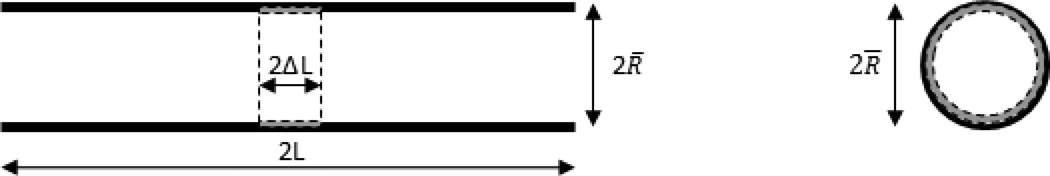
In the following we consider two idealized examples that allow all relevant quantities to be determined analytically and thus to be compared easily with numerical simulations. A homogeneous, thin-walled, axisymmetric cylindrical vessel of radius R̅ and length 2L is fixed in the axial direction on both ends. The vessel consists of one axial and one circumferential collagen fiber family, circumferential smooth muscle, and an isotropic elastin matrix. Elastin is assumed to exhibit no mass turnover and thus belongs to material group 𝕊₀. In contrast, smooth muscle and collagen fibers are assumed to exhibit the same turnover time constant τ and thus to form a second material group 𝕊₁. The mechanical behavior of elastin is modeled as neo-Hookean and that of collagen and smooth muscle as Fung exponentials (cf. equations (2.6) – (2.8) in [16] with material parameters and prestresses according to table 1 there), with a mass density ϱ = 1050 kg/m³ for all species. The initial areal mass density M̅ is uniform all over the vessel. Note that the parameters taken from [16] resemble the situation in the human abdominal aorta whereas the chosen collagen fiber families, an orthogonal grid of axial and circumferential fibers, rather mimic collagen alignment in muscular arteries and veins [17]. This idealized (hybrid) situation was chosen because the present theory of mechanobiological stability neglects the effects of wall shear stress on G&R and thus seems more applicable to elastic arteries (like the aorta) than to muscular arteries, whereas the choice of only one axial and one circumferential fiber family (rather than a helical fiber reinforcement as typical for elastic arteries) allows a simple, analytical treatment of both axial and circumferential instability in section 6.1 and section 6.2. A discussion of mechanobiological stability on the basis of more realistic vessel models will be presented in future work.

All quantities in the following example are expressed in (axial, radial, and circumferential) cylindrical coordinates (z, r, φ), which denote as subscripts components of vectors or tensors. The vessel domain in the initial configuration is the surface

$$\mathrm{\Omega }=\{(z,r,\phi ):z\epsilon [-L/2,L/2],r=\mathrm{R̅},\phi \epsilon [0,2\pi [\}.$$ (56)

The vessel is subject to a constant internal pressure p. Thus, generalized internal and external force vectors in (12) become with (A2) in Appendix A

$${\mathit{f}}_{\mathit{\text{int}}}=\left(\begin{array}{c}\hfill \partial T_{zz}/\partial z+\partial T_{z\phi }/\partial \phi \hfill \\ \hfill \partial T_{\phi z}/\partial z+T_{\phi \phi }/\partial \phi \hfill \\ \hfill -T_{\phi \phi }/R\hfill \end{array}\right)=\left(\begin{array}{c}\hfill \partial T_{zz}/\partial z\hfill \\ \hfill 0\hfill \\ \hfill -T_{\phi \phi }/R\hfill \end{array}\right),{\mathit{f}}_{\mathit{\text{ext}}}=\left(\begin{array}{c}\hfill 0\hfill \\ \hfill 0\hfill \\ \hfill p\hfill \end{array}\right),$$ (57)

because curvature in the axial direction equals zero. Here, T_zz, T_zφ, and T_φφ are components of the membrane stress tensor, with T_zφ = T_φz = 0 and ∂T_φφ/∂φ = 0 because of the assumed axisymmetry.

6.1 Axial G&R of a homogeneous vessel after a small lesion

In the first example, areal mass density is assumed to be zero for elastin, but greater than zero and initially uniform all over the vessel for axial collagen fibers. At time t = 0, the areal mass density of the axial collagen fibers is reduced in the region z ε[−ΔL, ΔL], with ΔL ≪ L, by a uniform small perturbation δM(0)(cf. Figure 1), which initiates axial G&R governed by the axial collagen fibers as there is no other species in this direction and all other directions remain unaffected. We thus focus on the axial direction and drop indices for species referring always to axial collagen for the remainder of this example. The (axial) generalized internal and external forces from (12) become

$${(f_{\mathit{\text{int}}})}_z=\partial T_{zz}/\partial z,{(f_{\mathit{\text{ext}}})}_z=0.$$ (58)

Figure 1.

Illustration of examples in section 6.1 and 6.2: Cross section through a vessel parallel to its long axis with axial collagen fibers removed in the central region as in example 6.1 (left). Cross section perpendicular to the long axis with circumferential elastin damage as described in example 6.2 (right). The perturbed regions are delimited by dashed lines, with the removed mass denoted by grey and the mass after perturbation denoted by black.

Thus T_zz is constant over the domain and the Cauchy stress (and also strain) is therefore constant in the two subdomains |z̅| < ΔL and ΔL < |z̅| < L (within which mass density is uniform), respectively. Due to symmetry with respect to z̅ = 0, we focus on the half-domain 0 ≤ z̅ ≤ ΔL. There, the displacement variation in z-direction is

$$\delta x_z=\{\begin{array}{cc}\hfill \mathrm{z̅}<\mathrm{\Delta }L:\hfill & \hfill \mathrm{\delta }ẑ\frac{\mathrm{z̅}}{\mathrm{\Delta }L}\hfill \\ \hfill \mathrm{\Delta }L<\mathrm{z̅}<L:\hfill & \hfill \delta ẑ\frac{L-\mathrm{z̅}}{\mathrm{L}-\mathrm{\Delta }L}\hfill \end{array},\delta {\epsilon }_{zz}=\{\begin{array}{cc}\hfill \mathrm{z̅}<\mathrm{\Delta }L:\hfill & \hfill \delta ẑ\frac{1}{\mathrm{\Delta }L}\hfill \\ \hfill \mathrm{\Delta }L<\mathrm{z̅}<L:\hfill & \hfill -\delta ẑ\frac{1}{\mathrm{L}-\mathrm{\Delta }L}\hfill \end{array},$$ (59)

where δẑ is the displacement variation at z̅ = ΔL and the only relevant displacement degree of freedom in the system. With ΔL ≪ L, we can neglect variations in strain, and thus stress, within the subdomain ΔL < |z̅| < L and therefore neglect too the G&R processes in this subdomain. Hence, we can focus on the subdomain |z̅| < ΔL. There (axial) displacement, strain, and thus stress depend only on δẑ and can be treated as simple scalar functions rather than scalar fields with

$$\frac{\delta T_{zz}}{\delta {\epsilon }_{zz}}=\frac{1}{\varrho }(\mathrm{M̅}\frac{\delta {\sigma }_{zz}}{\delta {\epsilon }_{zz}}-\mathrm{M̅}{\mathrm{\sigma ̅}}_{zz}\frac{\delta J}{\delta {\epsilon }_{zz}})=\frac{\mathrm{M̅}}{\varrho }[{({\mathrm{C̅}}_{el})}_{zz}-{\mathrm{\sigma ̅}}_{zz}],\frac{\delta {\epsilon }_{zz}}{\delta ẑ}=1/\mathrm{\Delta }L$$ (60)

so that we can infer from (22)

$${(K_{\mathit{\text{tot}}})}_{zz}^{-1}\frac{\delta {(f_{\mathit{\text{int}}})}_z}{\delta T_{zz}}=-\frac{\delta ẑ}{\delta {(f_{\mathit{\text{int}}})}_z}\frac{\delta {(f_{\mathit{\text{int}}})}_z}{\delta T_{zz}}=-\frac{\delta ẑ}{\delta T_{zz}}=-\frac{\delta ẑ}{\delta {\epsilon }_{zz}}\frac{\delta {\epsilon }_{zz}}{\delta T_{zz}}=-\frac{\mathrm{\Delta }L\varrho }{\mathrm{M̅}[{({\mathrm{C̅}}_{el})}_{zz}-{\mathrm{\sigma ̅}}_{zz}]}$$ (61)

and with J = 1 + δε_zz, and thus δJ/δẑ = δε_zz/δẑ, as well as δT_zz/δJ = −T_zz additionally

$${(K_{\mathit{\text{tot}}})}_{zz}^{-1}{(K_{el})}_{zz}=\frac{-\frac{\delta {(f_{\mathit{\text{int}}})}_z}{\delta T_{zz}}\frac{\delta T_{zz}}{{(\delta {\epsilon }_{el})}_{zz}}\frac{\delta {\epsilon }_{zz}}{\delta ẑ}}{-\frac{\delta {(f_{\mathit{\text{int}}})}_z}{\delta T_{zz}}\frac{\delta T_{zz}}{{(\delta {\epsilon }_{el})}_{zz}}\frac{\delta {\epsilon }_{zz}}{\delta ẑ}-\frac{\delta {(f_{\mathit{\text{int}}})}_z}{\delta T_{zz}}\frac{\delta T_{zz}}{\delta J}\frac{\delta J}{\delta ẑ}}=\frac{{({\mathrm{C̅}}_{el})}_{zz}}{{({\mathrm{C̅}}_{el})}_{zz}-{\mathrm{\sigma ̅}}_{zz}}.$$ (62)

With (61) and δT_zz/δM = σ̅_zz/ϱ we can rewrite (24) as

$$\delta {ẑ}_{el}(t=0^{+})=-\frac{\mathrm{\Delta }L{\mathrm{\sigma ̅}}_{zz}}{\mathrm{M̅}[{({\mathrm{C̅}}_{el})}_{zz}-{\mathrm{\sigma ̅}}_{zz}]}\delta M(t=0^{+})$$ (63)

and with (62) we conclude from (34) that

$$\delta {ẑ}_{el}(t)=\mathit{\text{exp}}(-{𝓂}_{G\&R}^{\tau }t/\tau )\delta {ẑ}_{el}(t=0^{+})$$ (64)

with the normalized stability margin

$${𝓂}_{G\&R}^{\tau }=\frac{\tau k_{\sigma }\mathrm{M̅}{({\mathrm{C̅}}_{el})}_{zz}-\mathrm{M̅}{\mathrm{\sigma ̅}}_{zz}}{\mathrm{M̅}{({\mathrm{C̅}}_{el})}_{zz}-\mathrm{M̅}{\mathrm{\sigma ̅}}_{zz}}.$$ (65)

Thus, with (28) and (48)

$$\delta {ẑ}_{gr}(t)=\frac{1}{{𝓂}_{G\&R}^{\tau }}[1-\mathit{\text{exp}}(-{𝓂}_{G\&R}^{\tau }t/\tau )]\delta {ẑ}_{el}(t=0^{+})$$ (66)

$$\delta {ẑ}_{gr}(t\to \infty )=\frac{1}{{𝓂}_{G\&R}^{\tau }}\delta {ẑ}_{el}(t=0^{+})$$ (67)

$${𝒜}_x=\frac{1}{{𝓂}_{G\&R}^{\tau }}$$ (68)

And, with (25), (60), (63) and (64), the (scalar) axial collagen areal mass density

$$\delta M(t)=\frac{1}{\tau k_{\sigma }{({\mathrm{C̅}}_{el})}_{zz}-{\mathrm{\sigma ̅}}_{zz}}[\tau k_{\sigma }{({\mathrm{C̅}}_{el})}_{zz}\mathit{\text{exp}}(-{𝓂}_{G\&R}^{\tau }t/\tau )-{\mathrm{\sigma ̅}}_{zz}]\delta M(t=0^{+})$$ (69)

$$\delta M(t\to \infty )=-\frac{{\mathrm{\sigma ̅}}_{zz}}{\tau k_{\sigma }{({\mathrm{C̅}}_{el})}_{zz}-{\mathrm{\sigma ̅}}_{zz}}\delta M(t=0^{+})$$ (70)

$${𝒜}_M=\frac{{\Vert \delta M(t\to \infty )\Vert }_2}{{\Vert \delta M(t=0^{+})\Vert }_2}=\left|\frac{{\mathrm{\sigma ̅}}_{zz}}{\tau k_{\sigma }{({\mathrm{C̅}}_{el})}_{zz}-{\mathrm{\sigma ̅}}_{zz}}\right|$$ (71)

The normalized stability margin ${𝓂}_{G\&R}^{\tau }$ obviously increases monotonically with τk_σ, which is consistent with Proposition 4. Moreover, (68) is consistent with Proposition 6 and (71) with Proposition 7.

This analytical solution was compared with numerical simulations in MATLAB. To this end, G&R and deformation after an initial perturbation of 0.01% of the axial collagen areal mass density was simulated similarly to [16] but without a finite element discretization in space as there was only one spatial degree of freedom δẑ in our example. Using a time step size Δt = 10⁻²τ, results in Figure 2 show an excellent agreement between the simulation and the above derived analytical solution. Note in the lower right plot of Figure 2 that even for a positive stability margin there remains a residual deformation, which becomes larger for smaller values of 𝓂_G&R, as expected from (48). For ${𝓂}_{G\&R}^{\tau }=3.4\times {10}^{-3}\approx 0$ we observe a nearly linear increase of the total deformation as expected because in this case the elastic deformation remains almost constant over time giving rise to a nearly constantly growing inelastic deformation according to (28). For negative 𝓂_G&R unstable exponential deformation is observed as expected.

Figure 2.

Comparison between simulation (crosses) and analytical solution (continued lines) for example in section 6.1: elastic (upper left) and inelastic (upper right) deformations and areal mass density (lower left) after perturbation for τk_σ = 1.5, 𝓂_G&R = 1.5/τ, total deformation for different stability margins (lower right)

6.2 Uniform circumferential G&R of a homogeneous vessel

In this second example, R̅ = 1.25 cm and the a real mass densities were assumed to be 0.34 kg/m², 0.22 kg/m², 0.60 kg/m² and 0.30 kg/m² for elastin, circumferential smooth muscle, circumferential and axial collagen fibers, similar to the human aorta studied in [16], with mean blood pressure p = 93 mmHg. At time t = 0, a small fraction of the elastin layer was uniformly removed throughout the vessel as a perturbation of the mass field so that the whole vessel experienced a uniform dilation δR of the radius without axial deformation. This situation mimics aging. The only non-zero variation in strain is

$$\delta {\epsilon }_{\phi \phi }=\frac{\delta R}{\mathrm{R̅}}$$ (72)

and the only relevant components in (57) are

$${(f_{\mathit{\text{int}}})}_r=-\frac{{\mathrm{T}}_{\phi \phi }}{R},{(f_{\mathit{\text{ext}}})}_r=p=\frac{{\sum }_{i=1}^n{\mathrm{M̅}}^i{\mathrm{\sigma ̅}}^i}{\mathrm{J̅}\mathrm{R̅}\varrho }.$$ (73)

From (57) and (72), and noting that δ(f_ext)_r/δR = 0 and δJ/δR = 1/R̅, we find around the initial mechanobiologically static state,

$${\left(K_{\mathit{\text{geo}}}\right)}_{rr}=-{\frac{\delta {(f_{\mathit{\text{int}}})}_r}{\delta R}|}_{\delta R_{el}=0}=-2\frac{{\sum }_{i=1}^n{\mathrm{M̅}}^i{\mathrm{\sigma ̅}}^i}{{\mathrm{R̅}}^2\varrho }$$ (74)

where the factor of two comes from adding contributions of decreased curvature and decreased wall thickness during dilation δR. In (74) we dropped the lower indices φφ on σ̅ⁱ and will similarly do so in the following for the elastic stiffnesses ${\mathrm{C̅}}_{el}^i$ since only the circumferential component matters. With δ(f_int)_r/δT_φφ = −1/R̅ and δε_φφ/δR = 1/R̅, we arrive at

$${(K_{el})}_{rr}=\frac{{\sum }_{i=1}^n{\mathrm{M̅}}^i{\mathrm{C̅}}_{el}^i}{{\mathrm{R̅}}^2\varrho },{(K_{\mathit{\text{tot}}})}_{rr}=\frac{{\sum }_{i=1}^n{\mathrm{M̅}}^i({\mathrm{C̅}}_{el}^i-2{\mathrm{\sigma ̅}}^i)}{{\mathrm{R̅}}^2\varrho }.$$ (75)

Note that δ(f_ext)_r/δR = 0 because (12) refers to the (respective current) spatial configuration in which the out-of-plane pressure load on the membrane remains constant. The system studied is an SETT system, hence the sum in (34) runs over only one index value J = 1. Then with (73), (74) and (75) we can rewrite (24), (34) and (36) as

$$\delta R(t=0^{+})=\delta R_{el}(t=0^{+})=-\frac{\mathrm{R̅}}{{\sum }_{i=1}^n{\mathrm{M̅}}^i({\mathrm{C̅}}_{el}^i-2{\mathrm{\sigma ̅}}^i)}\sum _{i=1}^n{\mathrm{\sigma ̅}}^i\delta M^i(t=0^{+}),$$ (76)

$$\delta {Ṙ}_{el}=-\frac{\tau {\sum }_{j\in {𝕊}_1}{\mathrm{M̅}}^j{k}_{\sigma }^j{\mathrm{C̅}}_{el}^j+{\mathrm{M̅}}^e{\mathrm{C̅}}_{el}^e-2{\sum }_{i=1}^n{\mathrm{M̅}}^i{\mathrm{\sigma ̅}}^i}{\tau {\sum }_{i=1}^n{\mathrm{M̅}}^i({\mathrm{C̅}}_{el}^i-2{\mathrm{\sigma ̅}}^i)}\delta R_{el},$$ (77)

and thus

$$\delta R_{el}(t)=\mathit{\text{exp}}(-{𝓂}_{G\&R}^{\tau }t/\tau )\delta R_{el}(t=0^{+})$$ (78)

with the (radial) stability margin

$${𝓂}_{G\&R}^{\tau }=\frac{\tau {\sum }_{j\in {𝕊}_1}{\mathrm{M̅}}^j{k}_{\sigma }^j{\mathrm{C̅}}_{el}^j+{\mathrm{M̅}}^e{\mathrm{C̅}}_{el}^e-2{\sum }_{i=1}^n{\mathrm{M̅}}^i{\mathrm{\sigma ̅}}^i}{{\sum }_{i=1}^n{\mathrm{M̅}}^i({\mathrm{C̅}}_{el}^i-2{\mathrm{\sigma ̅}}^i)},$$ (79)

where the upper index “e” is in this section reserved for elastin. Time integration of (78) used in (28) yields

$$\delta R_{gr}(t)=\frac{1}{{𝓂}_{G\&R}^{\tau }}[1-\mathit{\text{exp}}(-{𝓂}_{G\&R}^{\tau }t/\tau )]\delta R_{el}(t=0^{+}),$$ (80)

$$\delta R_{gr}(t\to \infty )=\frac{1}{{𝓂}_{G\&R}^{\tau }}\delta R_{el}(t=0^{+}),$$ (81)

and (45), assuming the system is stable,

$${𝒜}_x=\left|\frac{1}{{𝓂}_{G\&R}^{\tau }}\right|.$$ (82)

Using (76), (78) and (79) in (25) gives

$$\delta {Ṁ}^j(t)=-\frac{{\mathrm{M̅}}^j{k}_{\sigma }^j{\mathrm{C̅}}_{el}^j}{{\mathrm{\sigma ̅}}^j{\sum }_{i=1}^n{\mathrm{M̅}}^i({\mathrm{C̅}}_{el}^i-2{\mathrm{\sigma ̅}}^i)}\mathit{\text{exp}}(-{𝓂}_{G\&R}t)\sum _{i=1}^n{\mathrm{\sigma ̅}}^i\delta M^i(t=0^{+}),$$ (83)

and after time integration

$$\delta M^j(t)=\frac{{\mathrm{M̅}}^j{k}_{\sigma }^j{\mathrm{C̅}}_{el}^j}{{𝓂}_{G\&R}{\mathrm{\sigma ̅}}^j{\sum }_{i=1}^n{\mathrm{M̅}}^i({\mathrm{C̅}}_{el}^i-2{\mathrm{\sigma ̅}}^i)}[\mathit{\text{exp}}(-{𝓂}_{G\&R}t)-1]\sum _{i=1}^n{\mathrm{\sigma ̅}}^i\delta M^i(0^{+})+\delta M^j(0^{+}).$$ (84)

The stability condition for the system is ${𝓂}_{G\&R}^{\tau }>0$, which under the physiologically reasonable assumption that ${\mathrm{C̅}}_{el}^i>{\mathrm{\sigma ̅}}^i$ is, according to (79), equivalent to

$$\tau \sum _{j\in {𝕊}_1}{\mathrm{M̅}}^j{k}_{\sigma }^j{\mathrm{C̅}}_{el}^j+{\mathrm{M̅}}^e{\mathrm{C̅}}_{el}^e-2\sum _{i=1}^n{\mathrm{M̅}}^i{\mathrm{\sigma ̅}}^i>0.$$ (85)

This result confirms the positive impacts of increased elastic stiffness ${\mathrm{C̅}}_{el}^j$, gain factor $k_{\sigma }^j$, and turnover time τ on the mechanobiological stability shown theoretically in Proposition 3, Proposition 4, and Proposition 5.

Blood vessels are typically assumed to be at least mechanically stable. Otherwise, they would incidentally rupture or deform significantly from their preferred cylindrical shape and preferred size. Nevertheless, they may lose their mechanobiological stability at some time. As seen from (79), this instability may result from a loss of elastin or a decreased capacity of collagen production (i.e., reduced k_σ) in our model. Once this happens, even minor perturbations that are common in the vasculature could lead to an unstable G&R process along with a potentially unbounded dilatation on the slow time scale defined by the characteristic time constant of mass turnover (cf. (78) and (80) in the case of ${𝓂}_{G\&R}^{\tau }<0$). It thus seems natural to study a neurysms as a potential consequence of such a mechanobiological instability. In fact, the stabilizing effects of an increased capacity of collagen production (i.e., increased $k_{\sigma }^j$) or increased elastic stiffness (i.e., increased ${\mathrm{C̅}}_{el}^j$) as predicted by our theory, and clearly visible in (79), has been observed clinically and experimentally in aneurysms [18, 19] and studied numerically using a G&R approach [16]. Our mechanobiological stability theory may serve as a theoretical basis to systematically harness and strengthen such observations in future therapies.

Remark 6: An interesting consequence of (85), given ${\mathrm{M̅}}^e{\mathrm{C̅}}_{el}^e-2{\sum }_{i=1}^n{\mathrm{M̅}}^i{\mathrm{\sigma ̅}}^i\approx -2\times {10}^{2}kPa<0$, is that mechanobiological stability is controlled by the parameters in the first term: if the gain factor, turnover time, or stiffnesses of the species subject to G&R processes decrease (increase) sufficiently, each system can be destabilized (stabilized). This insight may help us to understand better the initiation of aneurysms and may form a basis for future therapies as numerous interventions (e.g., inhibition of proteases or microRNAs) can affect the production rate and turnover time for collagen (i.e., k_σ and τ).

Remark 7: In (65) and (79), we see that prestress appears in the stability margin only in the sum over all M̅ⁱσ̅ⁱ, that is, indirectly via the membrane stress, which is consistent with Proposition 2. The membrane stress in (79) is determined by the external loading via (73) so that there is no way to change the stability margin for the given blood pressure by a modification of prestresses.

Remark 8: Perivascular support of blood vessels was neglected in the above examples. In general, this support can be modeled by a positive contribution K_peri to the external geometric stiffness −δf_ext/δx. The stability margin in (79) would then become

$${𝓂}_{G\&R}^{\tau }=\frac{\tau {\sum }_{j\in {𝕊}_1}{\mathrm{M̅}}^j{k}_{\sigma }^j{\mathrm{C̅}}_{el}^j+{\mathrm{M̅}}^e{\mathrm{C̅}}_{el}^e-2{\sum }_{i=1}^n{\mathrm{M̅}}^i{\mathrm{\sigma ̅}}^i+K_{\mathit{\text{peri}}}}{{\sum }_{i=1}^n{\mathrm{M̅}}^i({\mathrm{C̅}}_{el}^i-2{\mathrm{\sigma ̅}}^i)}.$$ (86)

That is, the stiffness arising from perivascular support has a stabilizing effect, which agrees with clinical experience and intuition.

Finally, for the example in this section we compared our theoretical predictions with numerical G&R simulations (in MATLAB) for various parameter combinations and found excellent agreement between theory and simulation as illustrated in Figure 3. Again, these biologically motivated but otherwise idealized examples were constructed primarily to enable numerical evaluations of the predictions of the current concepts. Future studies should now be pursued to consider (patho)physiological situations.

Figure 3.

Comparison between simulation (crosses) and analytical solution (continued lines) for example in section 6.2: elastic (upper left) and inelastic (upper right) deformations and areal mass density (lower left) after perturbation for τk_σ = 1.5, 𝓂_G&R = 1.5/τ, total deformation for different stability margins (lower right)

7 Conclusions

On the basis of Lyapunov’s stability theory, we generalized the concepts of equilibrium and stability from engineering mechanics to address mechanobiological systems subject to mass turnover, as, for example, blood vessels. We demonstrated in Corollary 1, the “Prestress Corollary”, that a generalized concept of mechanobiological equilibrium implies that new material must be deposited with a non-zero prestress during any turnover process, which explains its presence in the vasculature. Subsequently, we demonstrated in the Theorem on Vascular Mechanobiological Stability that blood vessels can maintain their geometry and properties over long periods despite small perturbations that are common in vivo if and only if they are stable both mechanically and mechanobiologically. While most human-made systems are designed to be asymptotically stable, and thus to return after minor perturbations to their operating point, we demonstrated in section 5 that mechanobiological stability in the vasculature follows the concept of neutral Lyapunov stability, which further allows vessels to adapt over time to a changing environment. Adaptivity is an essential feature of all living tissues.

On the basis of this conceptual framework we propose a change of paradigm: whereas aneurysms often appear to be mechanically stable [20], they may be understood in terms of mechanobiological instabilities. Future predictions of rupture risk should thus take into consideration not only geometry and wall stress, but also measures of mechanobiological stability. To derive such measures, we proposed a number of general propositions that reveal the impact of different parameters on the mechanobiological stability. In particular, we demonstrated that an increased characteristic gain factor k_σ (e.g., increased collagen production in dilated vessels), an increased characteristic time constant τ of mass turnover (e.g., decreased proteolytic insult), and an increased elastic stiffness (e.g., increased collagen cross-linking) all improve the mechanobiological stability. The characteristic time constant of mass turnover was furthermore shown to set a natural time scale for G&R. Although it must be non-zero, the exact magnitude of prestress had only an indirect impact on the mechanobiological stability if it remained constant during G&R. This does not exclude, however, a potential positive impact of increases in prestress in already perturbed systems.

It is hoped that these collective insights might help not only to understand the genesis of aneurysms, but also potentially to find new treatments focused on collagen production rate, turnover time, and stiffness, each of which one may be modified by appropriate interventions.

Appendix A

In (12), the mechanical balance equation for a membrane is given using generalized internal and external forces f_int and f_ext, which are defined in this appendix. The membrane is represented geometrically by a curved surface that can be parametrized by two (curvilinear) coordinates (u, ν). At each point of the membrane, a coordinate frame can be defined by the two in-plane tangent vectors along constant values of u and ν, and the cross product of these two vectors provides a third coordinate direction perpendicular on the membrane. Then

$${\mathit{f}}_{\mathit{\text{ext}}}=\left(\begin{array}{c}\hfill {\mathit{f}}_{\mathit{\text{ext}}}^{\Vert }\hfill \\ \hfill f_{\mathit{\text{ext}}}^{\perp }\hfill \end{array}\right)\epsilon {ℝ}^3,$$ (A1)

is simply the external force per unit membrane area consisting of the in-plane load vector ${\mathit{f}}_{\mathit{\text{ext}}}^{\Vert }\epsilon {ℝ}^2$ and the out-of-plane load $f_{\mathit{\text{ext}}}^{\perp }\epsilon ℝ$ perpendicular to the tangent vectors along constant values of u and ν. In membrane models of blood vessels, $f_{\mathit{\text{ext}}}^{\perp }$ typically equals the blood pressure and ${\mathit{f}}_{\mathit{\text{ext}}}^{\Vert }$ the wall shear stress. Equilibrium requires, according to eqs. (2.15) and (2.16) in [21], that

$$\underset{{\mathit{f}}_{\mathit{\text{int}}}}{\underbrace{\left(\begin{array}{c}\hfill \nabla \mathit{T}\hfill \\ \hfill -\mathbf{𝒮}:\mathit{T}\hfill \end{array}\right)}}+\left(\begin{array}{c}\hfill {\mathit{f}}_{\mathit{\text{ext}}}^{\Vert }\hfill \\ \hfill f_{\mathit{\text{ext}}}^{\perp }\hfill \end{array}\right)=(\begin{array}{c}\hfill \mathbf{0}\hfill \\ \hfill 0\hfill \end{array}).$$ (A2)

where ∇T is the divergence of the membrane stress tensor and 𝒮 the shape tensor (or second fundamental tensor) of the curved surface representing the membrane. Note that if w is a unit tangent vector to the membrane, then the curvature of the membrane in the section plane in which w lies is κ(t) = w𝒮w. The curvature computed with the shape operator will be positive if the angle between w and the third axis of the Cartesian frame is growing as w is convected along the curved surface in the direction it is pointing. Choosing u and ν such that the first two axes of the local coordinate frame are principal directions of the membrane stress tensor T, one understands that 𝒮: T is the sum of the products of the two principal membrane stresses times their respective principal curvatures, which has to counterbalance $f_{\mathit{\text{ext}}}^{\perp }$.

Note that, in general, not only does f_ext depend on the spatial configuration x, but via 𝒮 also f_int does, which has to be accounted for in variational calculations.

References

- 1.Wolinsky H, Glagov S. A lamellar unit of aortic medial structure and function in mammals. Circulation research. 1967;20:99–111. doi: 10.1161/01.res.20.1.99. [DOI] [PubMed] [Google Scholar]
- 2.Humphrey JD. Cardiovascular Solid Mechanics: Cells, issues, and Organs, Lightning Source, UKltd. 2002 [Google Scholar]
- 3.Fung YC. Biomechanics: Motion, Flow, Stress, and Growth, Springer. 1990 [Google Scholar]
- 4.Shadwick RE. Mechanical design in arteries. Journal of Experimental Biology. 1999;202:3305–3313. doi: 10.1242/jeb.202.23.3305. [DOI] [PubMed] [Google Scholar]
- 5.Wolinsky H. Long-term effects of hypertension on the rat aortic wall and their relation to concurrent aging changes: morphological and chemical studies. Circulation research. 1972;30:301–309. doi: 10.1161/01.res.30.3.301. [DOI] [PubMed] [Google Scholar]
- 6.Dajnowiec D, Langille BL. Arterial adaptations to chronic changes in haemodynamic function: coupling vasomotor tone to structural remodelling. Clin Sci (Lond) 2007;113:15–23. doi: 10.1042/CS20060337. [DOI] [PubMed] [Google Scholar]
- 7.Chiquet M, Gelman L, Lutz R, Maier S. From mechanotransduction to extracellular matrix gene expression in fibroblasts. Biochimica et biophysica acta. 2009;1793:911–920. doi: 10.1016/j.bbamcr.2009.01.012. [DOI] [PubMed] [Google Scholar]
- 8.Li C, Xu Q. Mechanical stress-initiated signal transduction in vascular smooth muscle cells in vitro and in vivo. Cellular signalling. 2007;19:881–891. doi: 10.1016/j.cellsig.2007.01.004. [DOI] [PubMed] [Google Scholar]
- 9.Bersi MR, Ferruzzi J, Eberth JF, Gleason RL, Jr, Humphrey JD. Consistent biomechanical phenotyping of common carotid arteries from seven genetic, pharmacological, and surgical mouse models. Ann Biomed Eng. 2014;42:1207–1223. doi: 10.1007/s10439-014-0988-6. [DOI] [PMC free article] [PubMed] [Google Scholar]
- 10.Valentin A, Cardamone L, Baek S, Humphrey JD. Complementary vasoactivity and matrix remodelling in arterial adaptations to altered flow and pressure. J R Soc Interface. 2009;6:293–306. doi: 10.1098/rsif.2008.0254. [DOI] [PMC free article] [PubMed] [Google Scholar]
- 11.Figueroa CA, Baek S, Taylor CA, Humphrey JD. A Computational Framework for Fluid-Solid-Growth Modeling in Cardiovascular Simulations. Comput Methods Appl Mech Eng. 2009;198:3583–3602. doi: 10.1016/j.cma.2008.09.013. [DOI] [PMC free article] [PubMed] [Google Scholar]
- 12.Humphrey JD, Rajagopal KR. A constrained mixture model for growth and remodeling of soft tissues. Mathematical Models and Methods in Applied Sciences. 2002;12:407–430. [Google Scholar]
- 13.Baek S, Gleason RL, Rajagopal KR, Humphrey JD. Theory of small on large: Potential utility in computations of fluid–solid interactions in arteries. Comput Methods Appl Mech Eng. 2007;196:3070–3078. [Google Scholar]
- 14.Humphrey JD. Vascular adaptation and mechanical homeostasis at tissue, cellular, and sub-cellular levels. Cell biochemistry and biophysics. 2008;50:53–78. doi: 10.1007/s12013-007-9002-3. [DOI] [PubMed] [Google Scholar]
- 15.Schweizerhof K, Ramm E. Displacement dependent pressure loads in nonlinear finite element analyses. Computers & Structures. 1984;18:1099–1114. [Google Scholar]
- 16.Wilson JS, Baek S, Humphrey JD. Parametric study of effects of collagen turnover on the natural history of abdominal aortic aneurysms. Proc. R. Soc. A. 2013;469 doi: 10.1098/rspa.2012.0556. 20120556. [DOI] [PMC free article] [PubMed] [Google Scholar]
- 17.Cyron CJ, Humphrey JD. Preferred fiber orientations in healthy arteries and veins understood from netting analysis. Mathematics and Mechanics of Solids. 2014 in press. [Google Scholar]
- 18.Maegdefessel L, Azuma J, Toh R, Merk DR, Deng A, Chin JT, Raaz U, Schoelmerich AM, Raiesdana A, Leeper NJ, McConnell MV, Dalman RL, Spin JM, Tsao PS. Inhibition of microRNA-29b reduces murine abdominal aortic aneurysm development. J Clin Invest. 2012;122:497–506. doi: 10.1172/JCI61598. [DOI] [PMC free article] [PubMed] [Google Scholar]
- 19.Shantikumar S, Ajjan R, Porter KE, Scott DJ. Diabetes and the abdominal aortic aneurysm. Eur J Vasc Endovasc Surg. 2010;39:200–207. doi: 10.1016/j.ejvs.2009.10.014. [DOI] [PubMed] [Google Scholar]
- 20.Shah AD, Humphrey JD. Finite strain elastodynamics of intracranial saccular aneurysms. J Biomech. 1999;32:593–599. doi: 10.1016/s0021-9290(99)00030-5. [DOI] [PubMed] [Google Scholar]
- 21.Jenkins JT. The equations of mechanical equilibrium of a model membrane. SIAM J APPL MATH. 1977;32:755–764. [Google Scholar]