Occurrence and persistence of future atmospheric stagnation events

Abstract

Poor air quality causes an estimated 2.6 to 4.4 million premature deaths per year^1–3. Hazardous conditions form when meteorological components allow the accumulation of pollutants in the near-surface atmosphere^4–8. Global warming-driven changes to atmospheric circulation and the hydrological cycle^9–13 are expected to alter the meteorological components that control pollutant build-up and dispersal^5–8,14, but the magnitude, direction, geographic footprint, and public health impact of this alteration remain unclear^7,8. We utilize an air stagnation index and an ensemble of bias-corrected climate model simulations to quantify the response of stagnation occurrence and persistence to global warming. Our analysis projects increases in stagnation occurrence that cover 55% of the current global population, with areas of increase affecting 10 times more people than areas of decrease. By the late-21^st century, robust increases of up to 40 days per year are projected throughout the majority of the tropics and subtropics, as well as within isolated mid-latitude regions. Potential impacts over India, Mexico, and the western U.S. are particularly acute due to the intersection of large populations and increases in the persistence of stagnation events, including those of extreme duration. These results indicate that anthropogenic climate change is likely to alter the level of pollutant management required to meet future air quality targets.

Strategies to improve air quality typically focus on the reduction of emitted pollutants such as particulate matter (PM) and the precursors of tropospheric ozone (O₃). However, changing climate dynamics are also likely to play a role in determining future air quality, though the magnitude and direction of this role is uncertain^7,8. A recent assessment⁸ of meteorological influences found more frequent air stagnation to be the only meteorological condition that consistently resulted in higher near-surface concentrations of both PM and O₃. Given strong negative correlation between cyclone frequency and observed stagnation and pollution events^5–6 investigations of the response of air stagnation to enhanced radiative forcing have primarily focused on changes in cyclone frequency over regional (particularly U.S.) domains^{e.g.,5–6,15–16}. However, understanding of the response of future air stagnation events to elevated global warming has been found deficient due to inaccuracies in the simulation of meteorological variables relevant to air quality (“model bias”)^14,17, uncertainties in the spatial pattern of projected changes in those variables due to internal climate variability and/or model formulation^8,13–15,18, and lack of investigation of changes in stagnation event duration^14,18.

We examine air stagnation directly by applying a modified version of the Air Stagnation Index (ASI) to the CMIP5 global climate model ensemble. The ASI follows the ingredients-based approach of weather forecasting wherein fundamental components of a meteorological phenomenon are identified and analyzed using numerical models and/or observational datasets¹⁹. The ASI uses thresholds of daily precipitation and upper- and lower-atmospheric winds to determine when the atmosphere is likely to lack contaminant scavenging, horizontal dispersion, and vertical escape capabilities⁴ (see Methods). The daily co-occurrences of these meteorological conditions show a robust correlation with observed PM and O₃ pollution days^5–6, underpin operational air quality forecasts, and when persistent, are associated with extreme air pollution episodes^8,18. We utilize historical and high-emission scenario (RCP8.5) CMIP5 simulations to create a multi-model ensemble projection of air stagnation occurrence (see Supplemental Discussion). Our analysis examines changes in stagnation event duration, corrects model biases with six unique observational and reanalysis dataset combinations, and applies objective statistical analyses in conjunction with multi-model agreement criteria to quantify robustness of air stagnation change. Grid cell changes are considered robust if 66% of bias-corrected members pass a non-parametric permutation test at the 95% confidence level²⁰ and 66% agree on the change direction (See Methods).

Stagnant conditions are most frequent in the current climate over the tropics and sub-tropics, with areas of the western U.S., north Africa, central Asia, and Siberian Russia exhibiting relatively high occurrence in the mid-latitudes (Figure 1a). Regions that experience frequent stagnation but infrequent hazardous air quality, such as Siberian Russia²¹, confirm that the ASI measures potential impact: in the absence of human inhabitants or natural and/or anthropogenic pollutants, even ideal pollutant-accumulating meteorological conditions do not pose an air quality risk.

Figure 1. Characteristic changes in air stagnation and human exposure.

a, Mean annual baseline (1986–2005) stagnation days from the bias-corrected historical ensemble. b–d, Change in mean annual stagnation days from baseline to future periods (b 2016–2035, c 2046–2065 & d 2080–2099). White indicates <66% of ensemble members demonstrate significant change. Gray indicates >66% of members demonstrate significant change, but <66% of members agree on change direction. Blue (decreasing) or red (increasing) shades represent ensemble-mean changes, and indicate >66% of members demonstrate significant change and >66% agree on change direction. Bar plots show logarithmic values of the Air Stagnation Exposure Index, a metric that captures the potential human exposure to changes in stagnant conditions (Table S1). Vertical axes range from 10⁶–10^11.5 people·days yr⁻¹; note that over populated western U.S. grid cells, no robust air stagnation decreases are projected in future periods (ASEI = 0).

Robust increases in stagnation occurrence substantially outnumber decreases (Figure 1b–d). Changes in stagnation occurrence emerge in the early-21^st century over the western U.S. and many tropical and subtropical regions (Figure 1b). This regional signal intensifies as GHG concentrations rise over the 21^st century, such that by the late-century large portions of Amazonia, Mexico, and India are projected to experience 40+ more stagnation days per year (Figure 1d).

Model agreement in the direction of stagnation change is high, with Sahel Africa and the central Arabian Peninsula the only geographic regions lacking multi-model agreement in the sign of statistically significant change (Figure 1b–d). In some regions, including Mediterranean Europe, south-central China, and northern Australia, robust changes do not emerge until the late-21^st century, suggesting that the level of radiative forcing required to robustly alter stagnation-relevant meteorological components varies by region and depends on the magnitude and rate of GHG emissions. Robust decreases are few and isolated in the late-21^st century, with pockets of more-frequent pollutant-dispersing conditions over the southern Arabian Peninsula, central Argentina, South Africa, and eastern China (Figure 1d). No robust signal emerges over high northern latitudes, Saharan Africa, or most of Australia.

Changes in stagnation occurrence result from the cumulative responses of individual stagnation components (Figures 1–2). Increases in dry day occurrence dominate low- to mid-latitudes, while decreases are projected for high northern latitudes (Figure 2a). Changes in near-surface wind occurrences vary globally, with the western U.S. and northern India exhibiting the largest increases (Figure 2b). Stagnant mid-tropospheric winds predominantly increase, with the exception of isolated mid-latitude bands in each hemisphere (Figure 2c). Of the three components, the geographic footprint of multi-model agreement in the direction of significant change is smallest for near-surface winds, with disagreement over substantial portions of the tropics and subtropics (Figure S3).

Figure 2. Characteristic change in air stagnation components.

Change in mean annual stagnation conditions, future (2080–2099) minus baseline (1986–2005), for each Air Stagnation Index component. Signal not screened for statistical significance or multi-model agreement (for robust component changes see Figure S3). ASI component changes correspond to the ASI changes presented in Figure 1d (for non-robust ASI changes, see Figure S1). For component occurrence in the baseline period, see Figure S2.

Changes in stagnation occurrence can be driven by alteration of one, two, or all three components independently, or contemporaneously (Figures 1–2). Component changes vary both regionally and seasonally, and result from changes in atmospheric circulation and the hydrological cycle driven by enhanced radiative forcing^9–13. We identify three regions that exhibit robust stagnation increases, and highlight seasonal atmospheric changes that help to explain ASI component changes. Increases in autumn stagnation over India result primarily from increased dry day occurrence associated with weakened atmospheric ascent in the south (Figure S4) and increased mid-tropospheric stagnant wind occurrences associated with decreased zonal wind speeds in the north (Figures 3a–c & S5a–d)^9–11. Increases in spring stagnation over the south of China result from increased occurrence of each component, with increased dry day occurrence associated with a strengthening and northward shift in the descending branch of the Hadley circulation (Figures 3d–f & S5e–h)^9–10,12. Increases in spring stagnation over the Mediterranean result from more frequent dry day and near-surface stagnant wind occurrences, with more frequent dry days associated with enhanced mid-tropospheric subsidence (Figures 3g–i & S5i–l)^9–10.

Figure 3. Regional seasonal air stagnation changes.

Change in seasonal stagnation occurrence from baseline (1986–2005) to late-21^st century (2080–2099) over India (a) in fall (SON), China (d) in spring (MAM), and the Mediterranean (g) in spring. Baseline mean and baseline to late-21^st century mean change in mean zonal wind speeds [m s⁻¹] over India (b,c), meridional mass transport [10¹¹ kg sec⁻¹] over China (e,f), and mid-tropospheric (500 mb) vertical velocity (ω) [mb day⁻¹] over the Mediterranean (h,i). e,f Clockwise (cw) and counterclockwise (ccw) circulations indicated by color. f Dashed and solid white lines are baseline and future null mass transport isopleths.

Alteration of stagnation components will have the greatest impact where populations are high and sources of pollutants are plentiful. We introduce an air stagnation exposure index (ASEI) that (1) quantifies human exposure to daily stagnation events, (2) independently considers increases and decreases in future stagnation occurrence, and (3) focuses on the exposure of current populations through spatially-explicit year-2000 population counts²². Our ASEI does not consider future changes in population size or geographic distribution. Globally, the mean annual baseline ASEI is 405bn people·days/year. For scale, mean baseline ASEI for Guangzhou, China, a city of 12.8mil, is 0.52bn people·days. Observations²³ indicate that air quality over Guangzhou exceeded the PM_2.5 threshold on 36 days in 2010, suggesting annual-scale PM_2.5-pollution exposure of 0.46bn people·days, despite only implicit consideration of stagnation.

Bar charts in Figures 1b–d show global and regional changes in the logarithmic ASEI value (see Table S1 for non-logarithmic values). Regions of interest were selected based on factors such as pre-existing air quality problems, potential for substantial public health impacts due to high population exposure, and robust change in projected stagnation occurrence. Increases in stagnation exposure far surpass decreases, such that by the late-21^st century, the global sum of increased ASEI (77.7bn people·days/year) is 28 times larger than the sum of decreased ASEI (2.8bn people·days/year). Over half of the global ASEI increase is contributed by India (40.3bn people·days/year), with China (6.4bn people·days/year) and Mexico (2.8bn people·days/year) contributing changes an order of magnitude smaller (Figure 1d). Although negative ASEI changes exceed positive ASEI changes over the Mediterranean and eastern China in the early-21^st century, exposure increases surpass decreases in both regions by the late-century. Of the regions highlighted, the largest late-21^st century decrease in ASEI occurs in China (0.9bn people·days/year), which accounts for approximately 32% of the global decrease.

The potential public health impact increases as the duration of stagnation events lengthens²⁴. Multi-day stagnation episodes can lead to prolonged hazardous air exposure associated with extreme air pollution, severe outbreaks of acute cardiovascular and respiratory illness, and increased incidence of mortality^8,24–25. To determine the response of stagnation persistence to enhanced radiative forcing, we analyze the regional grid-cell ensemble distributions of stagnation occurrence, multi-day stagnation events, and average stagnation event length from the baseline and late-21^st century periods (Figure 4; see Figure S7 for component duration). In the western U.S., Mexico, and India all quantiles shift toward longer duration stagnation events in the late-21^st century, with the exception of the 5^th percentile over Mexico (Figure 4c). India exhibits the longest-duration events and the largest shift in persistence (Figure 4c), with almost 75% of late-21^st century events lasting longer than the baseline median. Increases in extreme duration events are greatest over Mexico, where 95^th percentile events shift from 4.9 days in the historical period to 5.8 days by the late-21^st century. Extreme stagnation event duration decreases over China, although the median length shows no appreciable change.

Figure 4. Baseline and late-21^st century stagnation day occurrences, multi-day events, and episode duration distributions.

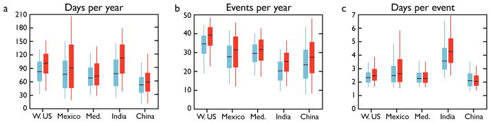
Ensemble distributions are created by compiling stagnation data from each grid cell within a region from each bias-corrected member. The baseline (1986–2005) period is depicted in blue and the future (2080–2099) in red. We conduct this analysis for each of the outlined regions in Figure 1 and indicate distribution medians (black lines), 25^th and 75^th percentiles (boxes), and 5^th and 95^th percentiles (line end-points).

Unlike air quality projections using Chemistry and Climate Models (CCMs)^e.g.,3,17,26, our stagnation projections do not explicitly account for pollutants. Rather, our results represent changes in the meteorological potential for the formation of hazardous air quality. Because GCMs are both more numerous and less computationally intensive than CCMs, our multi-GCM approach more fully captures the influence of natural atmospheric variability and model structural uncertainty²⁷. In addition, “off-line” analyses of stagnation conditions enables correction of systematic biases in the representation of meteorological variables that remain uncorrected in CCM air quality projections¹⁷. However, our focus on air quality meteorology without chemical transport does not quantify impacts on atmospheric pollutant concentrations, which are the ultimate determinant of air quality and associated health outcomes. A promising intermediate solution is to use bias-corrected fields from a large GCM ensemble to force offline Chemistry Transport Models, thereby quantifying transport, transformation, and capture of the spatial gradient of pollutants within the context of uncertainty in meteorological changes.

By quantifying the response of air quality meteorology to enhanced radiative forcing, our probabilistic analysis can provide important new information for efforts to protect public health by improving future air quality. This probabilistic analysis employs a rigorous climate change signal extraction process that corrects model biases, accounts for observational uncertainties, and tests for statistical significance and multi-model agreement. We find that continued global warming causes robust increases in the frequency and duration of air stagnation over several highly populated regions of the world, including multiple regions with severe pre-existing air quality problems. Our analysis highlights the importance of threshold-dependent impact metrics, such as the ASI and its constituent components, in quantifying uncertainty in the phenomena that most directly influence human systems²⁸. For example, analysis of events with similar/overlapping meteorological characteristics to stagnation episodes, including heat waves and droughts, suggests that an impact-focused examination of climatic processes within the multi-model framework can provide valuable – and distinct – information to those seeking to manage climate change risks²⁹.

Considering the strong links between air stagnation, air quality, and public health impacts, our results suggest that continued increases in GHG concentrations are likely to alter the atmosphere in ways that impact efforts to protect public health.

Methods

We apply a modified version of the National Climatic Data Center ASI. A grid cell day is considered stagnant when daily-mean near-surface (10-m) wind speeds are < 3.2 m s⁻¹, daily-mean mid-tropospheric (500 mb) wind speeds are <13 m s⁻¹, and daily-mean precipitation accumulation is <1 mm¹⁴. The ASI does not explicitly incorporate all meteorological factors known to influence air quality, including, relative humidity, temperature, turbulent mixing, and orographic barriers. Consequently, ASI component threshold sensitivities may vary locally/regionally and factors in addition to, or exclusive of, air stagnation may play a substantial role in determining local/regional air quality¹⁴.

Global warming-driven stagnation changes are explored using an ensemble of realizations from 15 modeling groups that provide requisite daily three-dimensional atmospheric fields from both Historical and RCP8.5 experiments of the Climate Model Intercomparison Project Phase 5 (Table S2). Because the ASI is reliant on absolute thresholds, systematic errors in CMIP5-simulated stagnation-relevant variables are bias corrected using an empirical quantile mapping technique^14,28,30. To account for observational uncertainties, we use a suite of six unique reanalysis and observational dataset combinations (see Supplemental Discussion). For wind correction, we use monthly NCEP-DOE R2 and ECMWF ERA-Interim reanalysis 500 mb and 10-m components. For precipitation, we use monthly University of Delaware v3.02 (UDel), Global Planetary Climatology Project v2.2 (GPCP), and Climate Prediction Center Merged Analysis of Precipitation (CMAP) data. Bias correction of the 15 CMIP5 models using six distinct combinations of observational standards forms what we refer to as the bias-corrected ensemble (90 members). For models with multiple realizations, we average all bias corrected realizations of each model prior to inclusion in the ensemble mean, such that each bias-corrected version of the model receives one vote (see Supplemental Discussion). All model, reanalysis, and observational data are interpolated to 0.5°×0.5°. To determine stagnation differences, the mean annual occurrence in three future RCP8.5 periods (2016–2035, 2046–2065, & 2080–2099) is compared to the baseline Historical period (1986–2005). Analysis of seasonal zonal wind speeds, meridional mass transport, and mid-tropospheric vertical velocity in Figures 3 and S4–6 utilize monthly-scale CMIP5 data and are not bias corrected.

Bias in native CMIP5 fields varies by component, magnitude, and location. Of the three ASI components, the magnitude of dry day (Figure S8a,e,i) and near-surface wind (Figure S8b,f,j) condition biases are greatest, while mid-tropospheric (500mb) wind conditions show both the least bias and greatest improvement from correction (Figure S8c,g,k). Baseline stagnation biases are greatest over high northern latitudes, northern Australia, and Amazonia, though our correction methodology substantially improves the mean occurrence (Figure S8d,h,l).

Extraction of a robust climate change signal from the bias-corrected ensemble follows a two-step process. First, statistical significance of the historic-to-future change in mean stagnation occurrence is assessed at each grid cell for each model using a non-parametric permutation test²⁰. For models with multiple realizations, statistical significance is assessed by comparing the combined population of historic realizations to that of the future. The permutation test makes no assumptions with regard to the data’s underlying distribution, thereby yielding greater confidence in the resulting conclusions. Following IPCC uncertainty guidance¹³, change is considered statistically robust if at least 66% of ensemble members demonstrate change at or above the 95% confidence level. Second, for those grid cells at which the simulated change is statistically robust, we assess ensemble member agreement in the direction of the simulated change.

If fewer than 66% of bias-corrected ensemble members exhibit change at or above the 95% confidence level, we plot the grid cell as white. If at least 66% of members exhibit change at or above the 95% confidence level, but fewer than 66% agree on the direction of the statistically significant changes, we plot the grid cell as gray. If at least 66% of members exhibit change at or above the 95% confidence level, and at least 66% agree on the direction of statistically significant changes, we consider the ASI-climate change signal robust, and plot ensemble-mean change in color (Figure 1). For comparison, late-century ensemble-mean air stagnation change without robustness screening is included as Figure S1. Stagnation changes presented in Figures 1 and S1 are largely in agreement with CMIP3-based results of Horton et al (14). Differences are attributable to added robustness screening, and changes in ensemble composition, model structure, emission scenarios, and reanalysis/observational datasets.

Use of multi-model ensembles to capture model design uncertainties and create probabilistic projections of future climate outcomes has become standard practice, due in part to the organizing efforts of CMIP. More recently, the air quality research community has adopted this protocol through independent efforts^e.g.,26 and under guidance from the Atmospheric Chemistry and Climate Model Intercomparison Project¹⁷. In our analysis, bias correction, consideration of the uncertainties inherent in observational standards, application of statistical rigor, and establishment of multi-model agreement thresholds all provide additional confidence in the multi-model probabilistic projection of the likelihood of future stagnation changes.

References

- 1.Anenberg SC, Horowitz LW, Tong DQ, West JJ. An estimate of the global burden of anthropogenic ozone and fine particulate matter on premature human mortality using atmospheric modeling. Environ Health Perspect. 2010;118:1189–1195. doi: 10.1289/ehp.0901220. [DOI] [PMC free article] [PubMed] [Google Scholar]
- 2.Lim SS, et al. A comparative risk assessment of burden of disease and injury attributable to 67 risk factors and risk factor clusters in 21 regions, 1990–2010: a systematic analysis for the Global Burden of Disease Study 2010. Lancet. 2012;380:2224–2260. doi: 10.1016/S0140-6736(12)61766-8. [DOI] [PMC free article] [PubMed] [Google Scholar]
- 3.Silva RA, et al. Global premature mortality due to anthropogenic outdoor air pollution and the contribution to past climate change. Environ Res Lett. 2013;8:034005. [Google Scholar]
- 4.Wang JXL, Angell JK. NOAA/Air Resources Laboratory ATLAS No 1. 1999. Air stagnation climatology for the United Sates (1948–1998) [Google Scholar]
- 5.Leibensperger EM, Mickley LJ, Jacob DJ. Sensitivity of US air quality to mid-latitude cyclone frequency and implications of 1980–2006 climate change. Atmos Chem Phys. 2008;8:7075–86. [Google Scholar]
- 6.Tai APK, Mickley LJ, Jacob DJ. Correlations between fine particulate matter (PM2.5) and meteorological variables in the United States: implications for the sensitivity of PM2.5 to climate change. Atmos Environ. 2010;44:3976–3984. [Google Scholar]
- 7.Jacob DJ, Winner DA. Effect of climate change on air quality. Atmos Environ. 2009;43:51–63. [Google Scholar]
- 8.Fiore AM, et al. Global air quality and climate. Chem Soc Rev. 2012;41:6663–6683. doi: 10.1039/c2cs35095e. [DOI] [PubMed] [Google Scholar]
- 9.Lu J, Vecchi GA, Reichler T. Expansion of the Hadley cell under global warming. Geophys Res Lett. 2007;34:L06805. [Google Scholar]
- 10.Held IM, Soden BJ. Robust responses of the hydrological cycle to global warming. J Clim. 2006;19:5686–5699. [Google Scholar]
- 11.Kripalani RH, Kumar P. Northeast monsoon rainfall variability over south peninsular India vis-à-vis the indian ocean dipole mode. Int J Clim. 2004;24:1267–1282. [Google Scholar]
- 12.Giorgi F, Lionello P. Climate change projections for the Mediterranean region. Glob Plan Ch. 2008;63:90–104. [Google Scholar]
- 13.Kirtman B, et al. Near-term Climate Change: Projections and Predictibility. In: Stocker TF, et al., editors. Climate Change 2013: The Physical Science Basis. IPCC, Cambridge Univ. Press; 2013. [Google Scholar]
- 14.Horton DE, Harshvardhan &, Diffenbaugh NS. Response of air stagnation frequency to anthropogenically enhanced radiative forcing. Environ Res Lett. 2012;7:044034. doi: 10.1088/1748-9326/7/4/044034. [DOI] [PMC free article] [PubMed] [Google Scholar]
- 15.Tai APK, et al. Meteorological modes of variability for fine particulate matter (PM2.5) air quality in the United States: implications for PM2.5 sensitivity to climate change. Atmos Chem Phys. 2012;12:3131–3145. [Google Scholar]
- 16.Turner AJ, Fiore AM, Horowitz LW, Bauer M. Summertime cyclones over the Great Lakes Storm Track from1860–2100: variability, trends, and association with ozone pollution. Atmos Chem Phys. 2013;13:565–578. [Google Scholar]
- 17.Lamarque JF, et al. The atmospheric chemistry and climate model Intercomparison project (ACCMIP): overview and description of models, simulations and climate diagnostics. Geosci Model Dev. 2013;6:179–206. [Google Scholar]
- 18.Dawson JP, Bloomer BJ, Winner DA, Weaver CP. Understanding the meteorological drivers of U.S. particulate matter. Bull Am Meteorol Soc. (in press) [Google Scholar]
- 19.Wetzel SW, Martin JE. An operational ingredient-based methodology for forecasting midlatitude winter season precipitation. Weather Forecast. 2001;16:156–167. [Google Scholar]
- 20.Singh D, Tsiang M, Rajaratnam B, Diffenbaugh NS. Observed changes in extreme wet and dry spells during the South Asian summer monsoon season. Nature Clim Change. (in press) [Google Scholar]
- 21.Brauer M, et al. Exposure assessment for estimation of the global burden of disease attributable to outdoor air pollution. Environ Sci Tech. 2011;46:652–660. doi: 10.1021/es2025752. [DOI] [PMC free article] [PubMed] [Google Scholar]
- 22.Center for International Earth Science Information Network (CIESIN) Socioeconomic Data and Applications Center (SEDAC): Gridded Population of the World, Version 3. Columbia University and Centro Internacional de Agricultura Tropical; Palisades, New York: 2005. available at http://sedac.ciesin.columbia.edu/ [Google Scholar]
- 23.Lui H, Wang XM, Pang JM, He KB. Feasibility and difficulties of China’s new air quality standard compliance: PRD case of PM2.5 and ozone from 2010 to 2025. Atmos Chem Phys. 2013;13:12013–12027. [Google Scholar]
- 24.Pope CA, III, Brook RD, Burnett RT, Dockery DW. How is cardiovascular disease mortality risk affected by duration and intensity of fine particulate matter exposure? An integration of the epidemiologic evidence. Air Qual Atmos Health. 2011;4:5–14. [Google Scholar]
- 25.Dockery DW, Pope CA., III Acute respiratory effects of particulate air pollution. Ann Rev Public Heath. 1994;15:107–132. doi: 10.1146/annurev.pu.15.050194.000543. [DOI] [PubMed] [Google Scholar]
- 26.Post ES, et al. Variation in estimated ozone-related health impacts of climate change due to modeling choices and assumptions. Environ Health Persp. 2012;120:1559–1564. doi: 10.1289/ehp.1104271. [DOI] [PMC free article] [PubMed] [Google Scholar]
- 27.Hawkins E, Sutton R. The potential to narrow uncertainty in regional climate predictions. Bull Am Meteorol Soc. 2009;90:1095–1107. [Google Scholar]
- 28.Diffenbaugh NS, Scherer M. Using climate impact indicators to evaluate climate model ensembles: temperature suitability of premium winegrape cultivation in the United States. Clim Dyn. 2013;40:709–729. [Google Scholar]
- 29.Seneviratne SI, et al. Changes in climate extremes and their impacts on the natural physical environment. In: Field CB, et al., editors. Managing the Risks of Extreme Events and Disasters to Advance Climate Change Adaptation. IPCC, Cambridge Univ. Press; 2012. [Google Scholar]
- 30.Ashfaq M, Bowling LC, Cherkauer K, Pal JS, Diffenbaugh NS. Influence of climate model biases and daily-scale temperature and precipitation events on hydrological impact assessments: a case study of the United States. J Geophys Res. 2010;115:D14116. [Google Scholar]
Associated Data
This section collects any data citations, data availability statements, or supplementary materials included in this article.