A Temporal Pattern Mining Approach for Classifying Electronic Health Record Data

Abstract

We study the problem of learning classification models from complex multivariate temporal data encountered in electronic health record systems. The challenge is to define a good set of features that are able to represent well the temporal aspect of the data. Our method relies on temporal abstractions and temporal pattern mining to extract the classification features. Temporal pattern mining usually returns a large number of temporal patterns, most of which may be irrelevant to the classification task. To address this problem, we present the Minimal Predictive Temporal Patterns framework to generate a small set of predictive and non-spurious patterns. We apply our approach to the real-world clinical task of predicting patients who are at risk of developing heparin induced thrombocytopenia. The results demonstrate the benefit of our approach in efficiently learning accurate classifiers, which is a key step for developing intelligent clinical monitoring systems.

1. INTRODUCTION

Advances in data collection and data storage technologies have led to the emergence of complex multivariate temporal datasets, where data instances are traces of complex behaviors characterized by multiple time series. Such data appear in a wide variety of domains, such as health care [Hauskrecht et al. 2010; Sacchi et al. 2007; Ho et al. 2003], sensor measurements [Jain et al. 2004], intrusion detection [Lee et al. 2000], motion capture [Li et al. 2009], environmental monitoring [Papadimitriou et al. 2005] and many more. Designing algorithms capable of learning from such complex data is one of the most challenging topics of data mining research.

This work primarily focuses on developing methods for analyzing electronic health records (EHRs). Each record in the data consists of multiple time series of clinical variables collected for a specific patient, such as laboratory test results, medication orders and physiological parameters. The record may also provide information about the patient’s diseases, surgical interventions and their outcomes. Learning classification models from this data is extremely useful for patient monitoring, outcome prediction and decision support.

The task of temporal modeling in EHR data is very challenging because the data is multivariate and the time series for clinical variables are acquired asynchronously, which means they are measured at different time moments and are irregularly sampled in time. Therefore, most times series classification methods (e.g, hidden Markov model [Rabiner 1989] or recurrent neural network [Rojas 1996]), time series similarity measures (e.g., Euclidean distance or dynamic time warping [Ratanamahatana and Keogh 2005]) and time series feature extraction methods (e.g., discrete Fourier transform, discrete wavelet transform [Batal and Hauskrecht 2009] or singular value decomposition [Weng and Shen 2008]) cannot be directly applied to EHR data.

This paper proposes a temporal pattern mining approach for analyzing EHR data. The key step is defining a language that can adequately represent the temporal dimension of the data. We rely on temporal abstractions [Shahar 1997] and temporal logic [Allen 1984] to define patterns able to describe temporal interactions among multiple time series. This allows us to define complex temporal patterns like “the administration of heparin precedes a decreasing trend in platelet counts”.

After defining temporal patterns, we need an algorithm for mining patterns that are important to describe and predict the studied medical condition. Our approach adopts the frequent pattern mining paradigm. Unlike the existing approaches that find all frequent temporal patterns in an unsupervised setting [Villafane et al. 2000; shan Kam and chee Fu 2000; Hoppner 2003; Papapetrou et al. 2005; Moerchen 2006; Winarko and Roddick 2007; Wu and Chen 2007; Sacchi et al. 2007; Moskovitch and Shahar 2009], we are interested in those patterns that are important for the classification task. We present the Minimal Predictive Temporal Patterns (MPTP) framework, which relies on a statistical test to effectively filter out non-predictive and spurious temporal patterns.

We demonstrate the usefulness of our framework on the real-world clinical task of predicting patients who are at risk of developing heparin induced thrombocytopenia (HIT), a life threatening condition that may develop in patients treated with heparin. We show that incorporating the temporal dimension is crucial for this task. In addition, we show that the MPTP framework provides useful features for classification and can be beneficial for knowledge discovery because it returns a small set of discriminative temporal patterns that are easy to analyze by a domain expert. Finally, we show that mining MPTPs is more efficient than mining all frequent temporal patterns.

Our main contributions are summarized as follows:

• —We propose a novel temporal pattern mining approach for classifying complex EHR data.
• —We extend our minimal predictive patterns framework [Batal and Hauskrecht 2010] to the temporal domain.
• —We present an efficient mining algorithm that integrates pattern selection and frequent pattern mining.

The rest of the paper is organized as follows. Section 2 describes the problem and briefly outlines our approach for solving it. Section 3 defines temporal abstraction and temporal patterns. Section 4 describes an algorithm for mining frequent temporal patterns and techniques we propose for improving its efficiency. Section 5 discusses the problem of pattern selection, its challenges and the deficiencies of the current methods. Section 6 introduces the concept of minimal predictive temporal patterns (MPTP) for selecting the classification patterns. Section 7 describes how to incorporate MPTP selection within frequent temporal pattern mining and introduces pruning techniques to speed up the mining. Section 8 illustrates how to obtain a feature-vector representation of the data. Section 9 compares our approach with several baselines on the clinical task of predicting patients who are at risk of heparin induced thrombocytopenia. Finally, Section 10 discusses related work and Section 11 concludes the paper.

2. PROBLEM DEFINITION

Let D = {<x_i, y_i >} be a dataset such that x_i ∈ X is the electronic health record for patient i up to some time t_i, and y_i ∈ Y is a class label associated 2 with a medical condition at time t_i. Figure 1 shows a graphical illustration of an EHR instance with 3 clinical temporal variables.

Fig. 1.

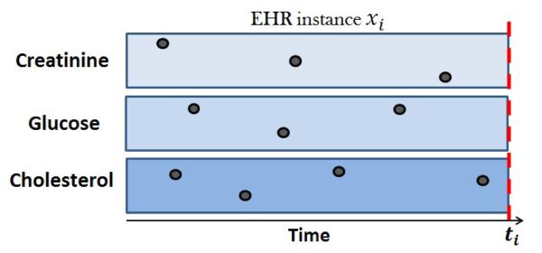
An example of an EHR data instance with three temporal variables. The black dots represent their values over time.

Our objective is to learn a function f: X → Y that can predict accurately the class labels for future patients. Learning f directly from X is very difficult because the instances consist of multiple irregularly sampled time series of different length. Therefore, we want to apply a transformation ψ : X → X′ that maps each EHR instance x_i to a fixed-size feature vector $x_i^{\prime }$ while preserving the predictive temporal characteristics of x_i as much as possible. One approach is to apply a static transformation and represent the data using a predefined set of features and their values as in [Hauskrecht et al. 2010]. Examples of such features are “most recent creatinine measurement”, “most recent creatinine trend”, “maximum cholesterol measurement”, etc. Our approach is different and we learn transformation ψ from the data using temporal pattern mining (dynamic transformation). This is done by applying the following steps:

1. Convert the time series variables into a higher level description using temporal abstraction.

2. Mine the minimal predictive temporal patterns Ω.

3. Transform each EHR instance x_i to a binary vector $x_i^{\prime }$, where every feature in $x_i^{\prime }$ corresponds to a specific pattern P ∈ Ω and its value is 1 if x_i contains P; and 0 otherwise.

After applying this transformation, we can use a standard machine learning method (e.g., SVM, decision tree, näive Bayes, or logistic regression) on {<$x_i^{\prime }$, y_i >} to learn function f.

3. TEMPORAL PATTERNS FROM ABSTRACTED DATA

3.1. Temporal Abstraction

The goal of temporal abstraction [Shahar 1997] is to transform the time series for all clinical variables to a high-level qualitative form. More specifically, each clinical variable (e.g., series of white blood cell counts) is transformed into an interval-based representation 〈v₁[b₁, e₁], …, v_n[b_n, e_n]〉, where v_i ∈ Σ is an abstraction that holds from time b_i to time e_i and Σ is the abstraction alphabet that represents a finite set of all permitted abstractions.

The most common types of clinical variables in EHR data are: medication administrations and laboratory results.

Medication variables are usually already represented in an interval-based format and specify the time interval during which a patient was taking a specific medication. For these variables, we simply use abstractions that indicate whether the patient is on the medication: Σ = {ON, OFF}.

Lab variables are usually numerical time series¹ that specify the patient’s laboratory results over time. For these variables, we use two types of temporal abstractions:

1. Trend abstraction that uses the following abstractions: Decreasing (D), Steady (S) and Increasing (I), i.e., Σ = {D, S, I}. In our work, we segment the lab series using the sliding window segmentation method [Keogh et al. 2003], which keeps expanding each segment until its interpolation error exceeds some error threshold. The abstractions are determined from the slopes of the fitted segments. For more information on trend segmentation, see [Keogh et al. 2003].

2. Value abstraction that uses the following abstractions: Very Low (VL), low (L), Normal (N), High (H) and Very High (VH), i.e., Σ = {VL, L, N, H, VH}. We use the 10th, 25th, 75th and 90th percentiles on the lab values to define these 5 states: a value below the 10th percentile is very low (VL), a value between the 10th and 25th percentiles is low (L), and so on.

Figure 2 shows the trend and value abstractions on a time series of platelet counts of a patient.

Fig. 2.

An example illustrating the trend and value abstractions. The blue dashed lines represent the 25th and 75th percentiles and the red solid lines represent the 10th and 90th percentiles.

3.2. State Sequence Representation

Let a state be an abstraction for a specific variable. For example, state E: V_i = D represents a decreasing trend in the values of temporal variable V_i. We sometimes use the shorthand notation D_i to denote this state, where the subscript indicates that D is abstracted from the i^th variable. Let a state interval be a state that holds during an interval. We denote by (E, b_i, e_i) the realization of state E in a data instance, where E starts at time b_i and ends at time e_i.

Definition 3.1. A state sequence is a series of state intervals, where the state intervals are ordered according to their start times²:

$$\langle (E_1,b_1,e_1),(E_2,b_2,e_2),\dots ,(E_l,b_l,e_l)\rangle :b_i\le e_i\wedge b_i\le b_{i+1}$$

Note that we do not require e_i to be less than b_i+1 because the states are obtained from multiple temporal variables and their intervals may overlap.

After abstracting all temporal variables, we represent every instance (i.e., patient) in the database as a state sequence. We will use the terms instance and state sequence interchangeably hereafter.

3.3. Temporal Relations

Allen’s temporal logic [Allen 1984] describes the relations for any pair of state intervals using 13 possible relations (see Figure 3). However, it suffices to use the following 7 relations: before, meets, overlaps, is-finished-by, contains, starts and equals because the other relations are simply their inverses. Allen’s relations have been used by most work on mining time interval data [shan Kam and chee Fu 2000; Hoppner 2003; Papapetrou et al. 2005; Winarko and Roddick 2007; Moskovitch and Shahar 2009].

Fig. 3.

Allen’s temporal relations.

Most of Allen’s relations require equality of one or two of the intervals end points. That is, there is only a slight difference between overlaps, is-finished-by, contains, starts and equals relations. Hence, when the time information in the data is noisy (not precise), which is the case in EHR data, using Allen’s relations may cause the problem of pattern fragmentation [Moerchen 2006]. Therefore we opt to use only two temporal relations, before (b) and co-occurs (c), which we define as follows: Given two state intervals E_i and E_j:

1. (E_i, b_i, e_i) before (E_j, b_j, e_j) if e_i < b_j, which is the same as Allen’s before relation.

2. (E_i, b_i, e_i) co-occurs with (E_j, b_j, e_j), if b_i ≤ b_j ≤ e_i, i.e. E_i starts before E_j and there is a nonempty time period where both E_i and E_j occur.

3.4. Temporal Patterns

In order to obtain temporal descriptions of the data, we combine basic states using temporal relations to form temporal patterns. Previously, we saw that the relation between two states can be either before (b) or co-occurs (c). In order to define relations between k states, we adopt Hoppner’s representation of temporal patterns [Hoppner 2003].

Definition 3.2. A temporal pattern is defined as P = (〈S₁, …, S_k〉, R), where S_i is the i^th state of the pattern and R is an upper triangular matrix that defines the temporal relations between each state and all of its following states:

$$R_{i,j}=S_{i}r{S}_j:i\in \{1,\dots ,k-1\}\wedge j\in \{i+1,\dots ,k\}\wedge r\in \{b,c\}$$

The size of pattern P is the number of states it contains. If size(P)=k, we say that P is a k-pattern. Hence, a single state is a 1-pattern (a singleton). We also denote the space of all temporal patterns of arbitrary size by TP.

Figure 4 graphically illustrates a 4-pattern with states 〈A₁, B₂, C₃, B₁, where the states are abstractions of temporal variables V₁, V₂ and V₃ using abstraction alphabet Σ = {A, B, C}. The half matrix on the right represents the temporal relations between every state and the states that follow it. For example, the second state B₂ is before the fourth state B₁: R_2,4 = b.

Fig. 4.

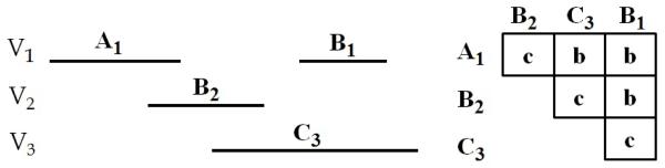
A temporal pattern with states 〈A₁, B₂, C₃, B₁〉 and temporal relations R_1,2 = c, R_1,3 = b, R_1,4 = b, R_2,3 = c, R_2,4 = b and R_3,4 = c.

Interesting patterns are usually limited in their temporal extensions, i.e., it would not be interesting to use the before relation to relate states that are temporally very far away from each other. Therefore, the definition of temporal patterns usually comes with a specification of a window size that defines the maximum pattern duration [Moerchen 2006; Hoppner 2003; Mannila et al. 1997].

In this paper, we are interested in the patient monitoring task, where we have the electronic health record for patient x_i up to time t_i and we want to decide whether or not patient x_i is developing a medical condition that we should alert physicians about. In this task, recent measurements of the clinical variables of x_i (close to t_i) are usually more predictive than distant measurements, as was shown by [Valko and Hauskrecht 2010]. The approach taken in this paper is to define windows of fixed width that end at t_i for every patient x_i and only mine temporal patterns that can be observed inside these windows.

Definition 3.3. Let T = 〈(E₁, b₁, e₁), …, (E_l, b_l, e_l)〉 be a state sequence that is visible within a specific window. We say that pattern P = (〈S₁, …, S_k〉, R) occurs in T (or that P covers T), denoted as P ∈ T, if there is an injective mapping π from the states of P to the state intervals of T such that:

$$(S_i=E_{\pi \left(i\right)})\wedge \left(\right(E_{\pi \left(i\right)},b_{\pi \left(i\right)},e_{\pi \left(i\right)}\left)R_{i,j}\right(E_{\pi \left(j\right)},b_{\pi \left(j\right)},e_{\pi \left(j\right)}\left)\right):\forall i\in \{1,\dots ,k\}\wedge j\in \{i+1,\dots ,k\}$$

Notice that checking the existence of a temporal pattern in a state sequence requires: (1) matching all k states of the patterns and (2) checking that all k(k − 1)/2 temporal relations are satisfied.

Definition 3.4. P = (〈S₁, …, S_k1〉, R) is a subpattern of $P^{\prime }=(\langle S_1^{\prime },\dots ,S_{k_2}^{\prime }\rangle ,R^{\prime })$, denoted as P ⊂ P′, if k₁ < k₂ and there is an injective mapping π from the states of P to the states of P′ such that:

$$S_i=S_{\pi \left(i\right)}^{\prime }\wedge R_{i,j}=R_{\pi \left(i\right),\pi \left(j\right)}^{\prime }\forall i\in \{1,\dots ,k_1\}\wedge j\in \{i+1,\dots ,k_1\}$$

For example, pattern (〈A₁, C₃〉,R_1,2 = b) is a subpattern of the pattern in Figure 4. If P is a subpattern of P′, we say that P′ is a superpattern of P.

Definition 3.5. The support of temporal pattern P in database D is the number of instances in D that contain P:

$$sup(P,D)=\mid \{T_i:T_i\in D\wedge P\in T_i\}\mid$$

Note that the support definition satisfies the Apriori property [Agrawal and Srikant 1994]:

$$\forall P,P^{\prime }\in TP\text{if}P\subset P^{\prime }\Rightarrow sup(P,D)\ge sup(P^{\prime },D)$$

We define a rule to be of the form P ⇒ y, where P is a temporal pattern and y is a specific value of the target class variable Y. We say that rule P ⇒ y is a subrule of rule P′ ⇒ y′ if P ⊂ P′ and y = y′.

Definition 3.6. The confidence of rule P ⇒ y is the proportion of instances from class y in all instances covered by P:

$$conf(P\Rightarrow y)=\frac{sup(P,D_y)}{sup(P,D)}$$

where D_y denotes all instances in D that belong to class y.

Note that the confidence of rule R:P ⇒ y is the maximum likelihood estimation of the probability that an instance covered by P belongs to)class y. If R is a predictive rule of class y, we expect its confidence to be larger than the prior probability of y in the data.

4. MINING FREQUENT TEMPORAL PATTERNS

In this section, we present our proposed algorithm for mining frequent temporal patterns. We chose to utilize the class information and mine frequent temporal patterns for each class label separately using local minimum supports as opposed to mining frequent temporal patterns from the entire data using a single global minimum support. The approach is reasonable when pattern mining is applied in the supervised setting because 1) for unbalanced data, mining frequent patterns using a global minimum support threshold may result in missing many important patterns in the rare classes and 2) mining patterns that are frequent in one of the classes (hence potentially predictive for that class) is more efficient than mining patterns that are globally frequent³.

The mining algorithm takes as input D_y: the state sequences from class y and σ_y: a user specified local minimum support threshold. It outputs all frequent temporal patterns in D_y:

$$\{P\in TP:sup(P,D_y)\ge {\sigma }_y\}$$

The mining algorithm performs an Apriori-like level-wise search [Agrawal and Srikant 1994]. It first scans the database to find all frequent 1-patterns. Then for each level k, the algorithm performs the following two phases to obtain the frequent (k+1)-patterns:

1. The candidate generation phase: Generate candidate (k+1)-patterns from the frequent k-patterns.

2. The counting phase: Obtain the frequent (k+1)-patterns by removing candidates with support less than σ_y.

This process repeats until no more frequent patterns can be found.

In the following, we describe in details the candidate generation algorithm and techniques we propose to improve the efficiency of candidate generation and counting.

4.1. Candidate Generation

We generate a candidate (k+1)-pattern by adding a new state (1-pattern) to the beginning of a frequent k-pattern⁴. Let us assume that we are extending pattern P = (〈S₁, …, S_k〉, R) with state S_new in order to generate candidates of the form ($(\langle S_1^{\prime },\dots ,S_{k_2}^{\prime }\rangle ,R^{\prime })$). First of all, we set $S_1^{\prime }=S_{new}$, $S_{i+1}^{\prime }=S_i$ for i ∈ {1, …, k} and $R_{i+1,j+1}^{\prime }=R_{i,j}$ for i ∈ {1, …, k − 1} ∧ j ∈ {i+1, …, k}. This way, we know that every candidate P′ of this form is a superpattern of P:P ⊂ P′.

In order to fully define a candidate, we still need to specify the temporal ˄ relations between the new state $S_1^{\prime }$ and states $S_2^{\prime },\dots ,S_{k+1}^{\prime }$, i.e., we should define $R_{1,i}^{\prime }$ for i ∈ {2, …, k + 1}. Since we have two possible temporal relations (before and co-occurs), there are 2^k possible ways to specify the missing relations. That is, 2^k possible candidates can be generated when adding a new state to a k-pattern. Let L denote all possible states (1-patterns) and let F_k denote the frequent k-patterns, generating the (k+1)-candidates naively in this fashion results in 2^k L F_k different candidates.

This large number of candidates makes the mining algorithm computationally very expensive and limits its scalability. Below, we describe the concept of incoherent patterns and introduce a method that smartly generates fewer candidates without missing any valid temporal pattern from the result.

4.2. Improving the Efficiency of Candidate Generation

Definition 4.1. A temporal pattern P is incoherent if there does not exist any valid state sequence that contains P.

Clearly, we do not have to generate and count incoherent candidates because we know that they will have zero support in the dataset. We introduce the following two propositions to avoid generating incoherent candidates when specifying the relations $R_{1,i}^{\prime }$ in candidates of the form $P^{\prime }=(\langle S_1^{\prime },\dots ,S_{k+1}^{\prime }\rangle ,R^{\prime })$.

Proposition 4.2. $P^{\prime }=(\langle S_1^{\prime },\dots ,S_{k+1}^{\prime }\rangle ,R^{\prime })$ is incoherent if $R_{1,i}^{\prime }=c$ and states $S_1^{\prime }$ and $S_i^{\prime }$ belong to the same temporal variable.

Two states from the same variable cannot co-occur because temporal abstraction segments each variable into non-overlapping state intervals.

Proposition 4.3. $P^{\prime }=(\langle S_1^{\prime },\langle ,S_{k+1}^{\prime }\rangle ,R^{\prime })$ is incoherent if $R_{1,j}^{\prime }=c\wedge \exists j<i:R_{1,j}^{\prime }=b$.

Proof. Let us assume that there exists a state sequence T = 〈(E₁, b₁, e₁), …, (E_l, b_l, e_l)〉 where P′ ∈ T. Let π be the mapping from the states of P′ to the state intervals of T. The definition of temporal patterns and the fact that state intervals in T are ordered by their start values implies that the matching state intervals 〈(E_π(1), b_π(1), e_π(1)), …, (E_π(k+1), b_π(k+1), e_π(k+1)) should also be ordered by their start times: b_π(1) ≤ … ≤ b_π(k+1). Hence, b_π(j) ≤ b_π(i). We also know that e_π(1) < b_π(j) because $R_{1,j}^{\prime }=b$. Therefore, e_π(1) < b_π(i). However, since $R_{1,i}^{\prime }=c$, then e_π(1) ≥ b_π(i), which is a contradiction. Therefore, there is no state sequence that contains P′.

Example 4.4. Assume we want to extend pattern P = (〈A₁, B₂, C₃, B₁〉, R) in Figure 4 with state C₂ to generate candidates of the form (〈C₂, A₁, B₂, C₃, B₁〉, R′). The relation between the new state C₂ and the first state A₁ is allowed to be either before or co-occurs: $R_{1,2}^{\prime }=b$ or $R_{1,2}^{\prime }=c$. However, according to proposition 4.2, C₂ cannot co-occur with B₂ because they both belong to temporal variable V₂ ($R_{1,3}^{\prime }\ne c$). Also, according to proposition 4.3, C₂ cannot co-occur with C₃ ($R_{1,4}^{\prime }\ne c$) because C₂ is before B₂ ($R_{1,3}^{\prime }=b$) and B₂ should start before C₃. For the same reason, C₂ cannot co-occur with B₁ ($R_{1,5}^{\prime }\ne c$). By removing incoherent patterns, we reduce the number of candidates that result from adding C₂ to 4-pattern P from 2⁴ =16 to only 2.

Theorem 4.5. There are at most k + 1 coherent candidates that result from extending a k-pattern with a new state.

Proof. We know that every candidate $P^{\prime }=(\langle S_1^{\prime },\dots ,S_{k+1}^{\prime }\rangle ,R^{\prime })$ corresponds to a specific assignment of $R_{1,i}^{\prime }\in \{b,c\}$. When we assign the temporal relations, once a relation before, all the following relations have to be before as well according to proposition 4.3. We can see that the relations can be co-occurs in the beginning of the pattern, but once we see a before relation at point q ∈ {2, …, k+1} in the pattern, all subsequent relations (i > q) should be before as well:

$$R_{1,i}^{\prime }=c:i\in \{2,\dots ,q-1\};R_{1,i}^{\prime }=b:i\in \{q,\dots ,k+1\}$$

Therefore, the total number of coherent candidates cannot be more than k +1, which is the total number of different combinations of consecutive co-occurs relations followed by consecutive before relations.

In some cases, the number of coherent candidates is less than k + 1. Assume that there are some states in P′ that belong to the same variable as state $S_1^{\prime }$. Let $S_j^{\prime }$ be the first such state (j ≤ k+1). According to proposition 4.2, $R_{1,j}^{\prime }\ne c$. In this case, the number of coherent candidates is j − 1 < k+1.

Corollary 4.6. Let L denote all possible states and let F_k denote all frequent k-patterns. The number of coherent (k+1)-candidates is always less or equal to (k + 1) × |L| × |F_k|.

So far we described how to generate coherent candidates by appending singletons to the beginning of frequent temporal patterns. However, we do not have to count all coherent candidates because some of them may be guaranteed not to be frequent. To filter out such candidates, we apply the Apriori pruning [Agrawal and Srikant 1994], which removes any candidate (k+1)-pattern if it contains an infrequent k-subpattern.

4.3. Improving the Efficiency of Counting

Even after eliminating incoherent candidates and applying the Apriori pruning, the mining algorithm is still computationally expensive because for every candidate, we need to scan the entire database in the counting phase to check whether or not it is a frequent pattern. The question we try to answer in this section is whether we can omit portions of the database that are guaranteed not to contain the candidate we want to count. The proposed solution is inspired by [Zaki 2000] that introduced the vertical format for itemset mining and later extended it to sequential pattern mining [Zaki 2001].

Let us associate every frequent pattern P with a list of identifiers for all state sequences in D_y that contain P:

$$P.id-list=\langle i_1,i_2,\dots ,i_n\rangle :T_{ij}\in D_y\wedge P\in T_{ij}$$

Clearly, sup(P, D_y) = {P.id-list}.

Definition 4.7. The potential id-list (pid-list) of pattern P is the intersection of the id-lists of its subpatterns:

$$P.pid-list={\cap }_{S\subset P}S.id-list$$

Proposition 4.8. ∀P ∈ TP: P.id-list ⊆ P.pid-list

Proof. Assume T_i is a state sequence in the database such that P ∈ T_i. By definition, i ∈ P.id-list. We know that T_i must contain all subpatterns of P according to the Apriori property: ∀S ⊂ P: S ∈ T_i. Therefore, ∀S ⊂ P: i ∈ S.id-list Ρ i ∈ ∩_S⊂P S.id-list = P.pid-list.

Note that for itemset mining, P.pid-list is always equal to P.id-list [Zaki 2000]. However, this is not true for time-interval temporal patterns. As an example, suppose P = (〈A₁, B₁, C₂〉, R_1,2 = b, R_1,3 = b, R_2,3 = c) and consider the state sequence T_i in Figure 5. T_i contains all subpatterns of P and hence i ∈ P.pid-list. However, T_i does not contain P (there is no mapping π that satisfies definition 3.3); hence i ≠ P.id-list.

Fig. 5.

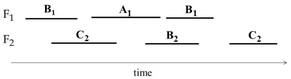
A state sequence that contains all subpatterns of pattern P = (〈A₁, B₁, C₂〉, R_1,2 = b, R_1,3 = b, R_2,3 = o), but does not contain P.

Putting it all together, we compute the id-lists in the counting phase (based on the true matches) and the pid-lists in the candidate generation phase. The key idea is that when we count a candidate, we only need to check the state sequences in its pid-list because:

$$i\notin P.pid-list\Rightarrow i\notin P.id-list\Rightarrow P\notin T_i,$$

This offers a lot of computational savings since the pid-lists get smaller as the size of the patterns increases, making the counting phase much faster.

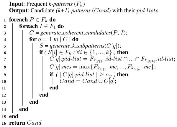
Algorithm 1 shows the candidate generation algorithm. After generating coherent candidates (line 3), we apply the Apriori pruning (lines 5 and 6). In our implementation, we hash all patterns in F_k, so that searching for the k-subpatterns of the candidate in F_k requires only k operations. Now that we found all k-subpatterns, we simply intersect their id-lists to compute the pid-list of the candidate (line 7). Note that the cost of the intersection is linear because the id-lists are always sorted according to the order of the instances in the database. Line 8 is used for mining the minimal predictive temporal patterns and will be explained later in Section 7. Finally, line 9 applies an additional pruning to remove candidates that are guaranteed not to be frequent according to the following implication of proposition 4.8:

$$\mid P.pid-list\mid <{\sigma }_y\Rightarrow \mid P.id-list\mid <{\sigma }_y\Rightarrow sup(P,D_y)<{\sigma }_y$$

ALGORITHM 1.

A high-level description of candidate generation.

5. SELECTING TEMPORAL PATTERNS FOR CLASSIFICATION

Applying frequent temporal pattern mining on data usually results in a very large number of patterns, most of which may be unimportant for the classification task. Using all of these patterns as features can hurt the classification performance due to the curse of dimensionality. Therefore, it is important to develop effective methods to select a small subset of patterns that are likely to improve the classification performance.

The task of pattern selection is more challenging than the well-studied task of feature selection due to the nested structure of patterns: if P is frequent, all instances covered by P are also covered by all of its subpatterns, which are also in the result of the frequent pattern mining method. This nested structure causes the problem of spurious patterns, which we will illustrate in the following.

5.1. Spurious Patterns

Definition 5.1. A temporal pattern P is a spurious pattern if P is predictive when evaluated by itself, but it is redundant given one of its subpatterns.

Example 5.2. Assume that having very low platelet counts (PLT) is an important risk factor for heparin induced thrombocytopenia (HIT). If we denote pattern PLT=VL by P, we expect conf (P ⇒ HIT) to be much higher than the HIT prior in the data. Now assume that there is no causal relation between the patient’s potassium (K) level and his risk of HIT, so a pattern like K=N (normal potassium) does not change our belief about the presence of HIT. If we combine these two patterns, for example P′:K=N before PLT=VL, we expect that conf (P′ ⇒ HIT) ≈ conf (P ⇒ HIT). The intuition behind this is that the instances covered by P′ can be seen as a random π sub-sample of the instances covered by P. So if the proportion of HIT cases in P is relatively high, we expect the proportion of HIT cases in P′ to be high as well [Batal and Hauskrecht 2010].

The problem is that if we examine P′ by itself, we may falsely conclude that it is a good predictor of HIT, where in fact this happens only because P′ contains the real predictive pattern P. Having such spurious patterns in the mining results is undesirable for classification because it leads to many redundant and highly correlated features. It is also undesirable for knowledge discovery because spurious patterns can easily overwhelm the domain expert and prevent him/her from understanding the real causalities in the data.

5.2. The Two-Phase Approach

The most common way to select patterns for classification is the two-phase approach, which generates all frequent patterns in the first phase and then selects the top k discriminative patterns in the second phase. This approach has been used by [Cheng et al. 2007; Li et al. 2001] for itemset based classification, by [Exarchos et al. 2008; Tseng and Lee 2005] for sequence classification and by [Deshpande et al. 2005] for graph classification. However, the two-phase approach is not very effective because when frequent patterns are evaluated individually in the second phase, there is a high risk of selecting spurious patterns because they look predictive using most interestingness measures [Geng and Hamilton 2006]. One way to partially overcome this problem is to apply an iterative forward pattern selection method as in [Cheng et al. 2007]. However, such methods are computationally very expensive when applied on large number of frequent patterns.

Having discussed these problems, we propose the minimal predictive temporal patterns framework for selecting predictive and non-spurious temporal patterns for classification.

6. MINIMAL PREDICTIVE TEMPORAL PATTERNS

Definition 6.1. A frequent temporal pattern P is a Minimal Predictive Temporal Pattern (MPTP) for class y if P predicts y significantly better than all of its subpatterns.

The MPTP definition prefers simple patterns over more complex patterns (the Occam’s Razor principal) because pattern P is not an MPTP if its effect on the class distribution “can be explained” by a simpler pattern that covers a larger population.

In order to complete the definition, we define the MPTP statistical significance test and explain how to address the issue of multiple hypothesis testing.

6.1. The MPTP Significance Test

Assume we want to check whether temporal pattern P is an MPTP for class y. Suppose that P covers N instances in the entire database D and covers N_y instances in D_y (the instances from class y). Let ${\widehat{\theta }}_{best}$ be the highest confidence achieved by any subrule of P ⇒ y:

$${\widehat{\theta }}_{best}=\underset{S\subset P}{\max }\left(conf\right(S\Rightarrow y\left)\right)$$

Let us denote the true underlying probability of observing y in group P by θ. We define the null hypothesis H₀ to be $\theta ={\widehat{\theta }}_{best}$. That is, H₀ says that N_y is generated from N according to the binomial distribution with probability ${\widehat{\theta }}_{best}$. The alternative hypothesis H₁ says that $\theta >{\widehat{\theta }}_{best}$ (a one sided statistical test). We compute the p-value of the MPTP significance test as follows:

$$p-value=P{r}_{binom}(x\ge N_y;N,{\widehat{\theta }}_{best})$$

This p-value can be interpreted as the probability of observing N_y or more instances of class y out of the N instances covered by P if the true underlying probability is ${\widehat{\theta }}_{best}$. If the p-value is smaller than a significance level (e.g., p-value < 0.01), then the null hypothesis H₀ is very unlikely. In this case, we reject H₀ in favor of H₁, which say that P ⇒ y is significantly more predictive than all its subrules, hence P is an MPTP.

This statistical test can filter out many spurious patterns. Going back to Example 5.2, we do not expect spurious pattern P′:K=N before PLT=VL to be an MPTP because it does not predict HIT significantly better that the real pattern: PLT=VL.

6.2. Correcting for Multiple Hypothesis Testing

When testing the significance of multiple patterns in parallel, it is possible that some patterns will pass the significance test just by chance (false positives). This is a concern for all pattern mining techniques that rely on statistical tests.

In order to tackle this problem, the significance level should be adjusted by the number of tests performed during the mining. The simplest way is the Bonferroni correction [shaffer 1995], which divides the significance level by the number of tests performed. However, this approach is very conservative (with large type II error) when the number of tests is large, making it unsuitable for pattern mining. In this work, we adopt the FDR (False Discovery Rate) technique [Benjamini and Hochberg 1995], which directly controls the expected proportion of false discoveries in the result (type I error). FDR is a simple method for estimating the rejection region so that the false discovery rate is on average less than α. It takes as input sorted p-values: p₍₁₎ ≤ p₍₂₎ … p_(m) and estimates k̂ that tells us that only hypotheses associated with p₍₁₎, p₍₂₎, …, p_(k̂) are significant. We apply FDR to post-process all potential MPTP (patterns satisfying the MPTP significance test) and select the ones that satisfy the FDR criteria.

7. MINING MINIMAL PREDICTIVE TEMPORAL PATTERNS

The algorithm in Section 4 describes how to mine all frequent temporal patterns for class y using D_y. In this section, we explain how to mine minimal predictive temporal patterns for class y. Our algorithm is integrated with frequent pattern mining in order to directly mine the MPTP set, as opposed to mining all frequent patterns first and then selecting MPTP as in the two-phase approach. To do this, the algorithm requires another input: D_¬y, which is the instances in the database D that do not belong to class y: D_¬y = D − D_y.

7.1. Extracting MPTPs

The process of testing whether temporal pattern P is an MPTP is not trivial because the definition demands checking P against all its subpatterns. That is, for a k-pattern, we need to compare it with all of its 2^k−1 subpatterns!

In order to avoid this inefficiency, we associate every frequent pattern P with two values:

1. P.mcs (Maximum Confidence of Subpatterns) is the maximum confidence of all subpatterns of P:

   $$P.mcs=\underset{S\subset P}{\max }\left(conf\right(S\Rightarrow y\left)\right)$$ (1)
2. P.mc (Maximum Confidence) is the maximum confidence of P and all of its subpatterns:

   $$P.mc=\max \left(conf\right(P\Rightarrow y),P.mcs)$$ (2)

Note that P.mcs is what we need to perform the MPTP significance test for pattern P. However, we need a way to compute P.mcs without having to access all subpatterns. The idea is that we can re-expressed P.mcs for any k-pattern using the maximum confidence values of its (k-1)-subpatterns:

$$P.mcs=\underset{S\subset P}{\max }(S.mc):size\left(S\right)=k-1$$ (3)

This leads to a simple dynamic programming type of algorithm for computing these two values. Initially, for every frequent 1-patterns P, we set P.mcs to be the prior probability of class y in the data and compute P.mc using expression (2). In the candidate generation phase, we compute mcs for a new candidate k-pattern using the mc values of its (k-1)-subpatterns according to expression (3) (Algorithm 1: line 8). Then, we compute the mc values for the frequent k-patterns in the counting phase, and repeat the process for the next levels.

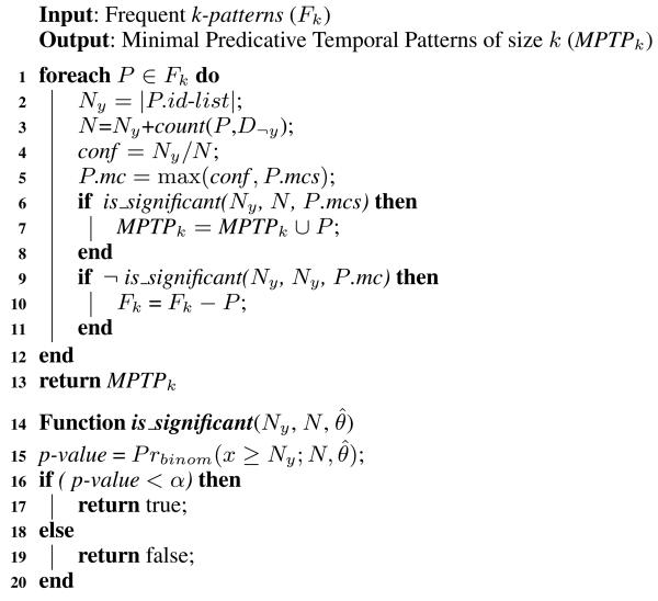
The algorithm for extracting the MPTP of size k from the frequent k-patterns is outlined in Algorithm 2. For every frequent pattern P, we compute P.mc (line 5). Then we add P to the MPTP set if it satisfies the MPTP significance test (lines 6 and 7).

ALGORITHM 2.

Extracting the MPTPs from the frequent k-patterns.

7.2. Pruning the Search Space

In this section, we illustrate how integrating MPTP selection with frequent temporal pattern mining helps pruning the search space (speeding up the mining). We say that temporal pattern P is pruned if we do not explore any of its superpatterns. Frequent pattern mining relies only on the supportinformation to prune infrequent patterns according to the Apriori property. That is, all patterns that are not frequent are pruned because their superpatterns are guaranteed not to be frequent.

In the following, we present two pruning techniques that can utilize the predictiveness of patterns to further prune the search space. The first technique is lossless, while the second is lossy.

7.2.1. Lossless Pruning

This section describes a lossless pruning technique that can prune parts of the search space without missing any MPTP. The idea is to prune pattern P if we guarantee that none of P’s superpatterns will be an MPTP. However, since the algorithm is applied in a level-wise fashion, we do not know the class distribution in the superpatterns of P. To overcome this difficulty, we define the optimal superpattern of P, denoted as P*, to be a hypothetical pattern that covers all and only the instances of class y in P, i.e., sup(P*, D_y) = sup(P, D_y) and sup(P*, D_¬y) = 0. Clearly, P cannot generate any superpattern that predicts y better than P*. Now, we prune P if P* is not an MPTP with respect to P.mc (the highest confidence achieved by P and its subpatterns). This pruning is outlined in Algorithm 2: lines 9 and 10. Note that this pruning is guaranteed not to miss any MPTP.

7.2.2. Lossy Pruning

This section describes a lossy pruning technique that speeds up the mining at the risk of missing some MPTPs. We refer to the patterns mined with the lossy pruning as A-MPTP (Approximated MPTP). The idea is to prune pattern P if it does not show any sign of being more predictive than its subpatterns. To do this, we simply perform the MPTP significance test, but at a higher significance level ₂ than the significance level used in the original MPTP significance test: α₂ ∈ [α, 1]. If P does not satisfy the test with respect to α₂, we prune P. We call α₂ the pruning significance level.

Note that α₂ is a parameter that controls the tradeoff between efficiency and completeness. So if we set α₂ = 1, we do not perform any lossy pruning. On the other end of the spectrum, if we set α₂ = α, we prune every non-MPTP pattern, which leads to very aggressive pruning!

Example 7.1. Assume that temporal pattern P covers 25 instances of class y and 15 instances that are not from class y and that the maximum confidence for P’s subpatterns is P.mcs = 0.65. If we apply the lossy pruning using pruning significance level α₂ = 0.5, we prune P because the p-value of the MPTP significance test is larger than α₂: P r_binom(x ≥ 25; 40, 0.65) = 0.69 > 0.5.

8. FEATURE SPACE REPRESENTATION

After we mine the MPTPs from each class label separately, we take the union of these patterns, denoted by Ω, to define the classification features. To do this, we transform each EHR instance x_i into a binary vector $x_i^{\prime }$ of size equal to |Ω|, where $x_{i,j}^{\prime }$ corresponds to a specific MPTP P_j and its value is 1 if P_j occurs in x_i; and 0 otherwise. Once the data is transformed to this binary representation, we can apply standard machine learning algorithms (e.g., SVM, decision tree, näive Bayes, or logistic regression) to learn the classification model.

9. EXPERIMENTAL EVALUATION

In this section, we test and present results of our temporal pattern mining approach on the problem of predicting patients who are at risk of developing heparin induced thrombocytopenia (HIT) [Warkentin 2000]. HIT is a pro-thrombotic disorder induced by heparin exposure with subsequent thrombocytopenia (low platelets in the blood) and associated thrombosis (blood clot). It is a life-threatening condition if it is not detected and managed properly. Hence, it is extremely important to detect the onset of the condition.

9.1. Dataset

We use data acquired from a database that contains 4,281 electronic health records of post cardiac surgical patients [Hauskrecht et al. 2010]. From this database, we selected 220 instances of patients who were considered by physicians to be at risk of HIT and 220 instances of patients without the risk of HIT. The patients at risk of HIT were selected using information about the heparin platelet factor 4 antibody (HPF4) test orders. The HPF4 test is ordered for a patient when a physician suspects the patient is developing HIT and hence it is a good surrogate of the HIT-risk label. The HIT-risk instances include clinical information up to the time HFP4 was ordered. The negative (no HIT-risk) instances were selected randomly from the remaining patients. These instances include clinical information up to some randomly selected time.

For every instance, we consider the following 5 clinical variables: platelet counts (PLT), activated partial thromboplastin time (APTT), white blood cell counts (WBC), hemoglobin (Hgb) and heparin orders. PLT, APTT, WBC and Hgb are numerical time series and we segment them using trend and value abstractions (Section 3.1). Heparin orders are already in an interval-based format that specifies the time period the patient was on heparin. We set the window size of temporal patterns to be the last 5 days of every patient record.

9.2. Classification Performance

In this section, we test the ability of our methods to represent and capture temporal patterns important for predicting HIT. We compare our methods, MPTP and its approximate version A-MPTP, to the following baselines:

1. Last_values: The features are the most recent value of each clinical variable. For example, the most recent value for PLT is 92, the most recent value for Hgb is 13.5, and so on.

2. Last_abs: The features are the most recent trend and value abstractions of each clinical variable. For example, the most recent trend abstraction for PLT is “decreasing”, the most recent value abstraction for PLT is “low”, and so on.

3. TP_all: The features are all frequent temporal patterns (without applying pattern selection).

4. TP_IG: The features are the top 100 frequent temporal patterns according to information gain (IG).

5. TP_chi: The features are the frequent temporal patterns that are statistically significant according to the χ² test with significance level α = 0.01. This method applies FDR to correct for multiple hypothesis testing.

The first two methods (1-2) are atemporal and do not rely on any temporal ordering when constructing their features. On the other hand, methods 3-5 use temporal patterns that are built using temporal abstractions and temporal logic. However, unlike MPTP and A-MPTP, they select the patterns using standard feature selection methods without considering the nested structure of the patterns.

We set the significance level = 0.01 for MPTP and A-MPTP, and we set the pruning significance level α₂ = 0.5 for A-MPTP (see Section 7.2.2). We set the local minimum supports to 10% of the number of instances in the class for all compared methods.

We judged the quality of the different feature representations in terms of their induced classification performance. More specifically, we use the features extracted by each method to build an SVM classifier and evaluate its performance using the classification accuracy and the area under the ROC curve (AUC).

In addition, we compared our methods to MBST (Model Based Search Tree) [Fan et al. 2008], a recently proposed method that combines frequent pattern mining and decision tree induction. MBST builds the decision tree as follows: for each node 1) invoke a frequent pattern mining algorithm; 2) select the most discriminative pattern according to IG; 3) divide the data into two subsets: one containing the pattern and the other not; and 4) repeat the process recursively on the two subsets. We extend this method to temporal pattern mining and refer to it in the results as to TP_MBST. We set the invocation minimum support to be 10%, i.e., at each node of the tree, the algorithm mines temporal patterns that appear in more than 10% of the instances in that node.

Table I shows the classification accuracy and the AUC for each of the methods. All classification results are reported using averages obtained via 10-folds cross validation.

Table I.

Classification Performance

Method	Accuracy	AUC
Last_values	78.41	89.57
Last_abs	80.23	88.43
TP_all	80.68	91.47
TP_IG	82.50	92.11
TP_chi	81.36	90.99
TP_MBST	83.5	89.85
MPTP	85.68	94.42
A-MPTP	85.45	95.03

The classification accuracy (%) and the area under the ROC curve (%) for different feature extraction methods.

The results show that temporal features generated using temporal abstractions and temporal logic are beneficial for predicting HIT, since they outperformed methods based on atemporal features. The results also show that the MPTP and A-MPTP are the best performing methods. Note that although the temporal patterns generated by TP_all, TP_IG, and TP_chi subsume or overlap MPTP and A-MPTP patterns, they also include many irrelevant and spurious patterns that negatively effect their classification performance.

Figure 6 shows the classification accuracy of the temporal pattern mining methods under different minimum support values. We did not include TP_MBST because it is very inefficient when the minimum support is low⁵. We can see that MPTP and A-MPTP consistently outperform the other methods under different settings of minimum support.

Fig. 6.

The classification accuracy of TP_all, TP_IG, TP_chi, MPTP and A-MPTP for different minimum supports.

9.3. Knowledge Discovery

In order for a pattern mining method to be useful for knowledge discovery, the method should provide the user with a small set of understandable patterns that are able to capture the important information in the data.

Figure 7 compares the number of temporal patterns (on a logarithmic scale) that are extracted by TP_all, TP_chi, MPTP and A-MPTP under different minimum support thresholds. Notice that the number of frequent temporal patterns (TP_all) exponentially blows up when we decrease the minimum support. Also notice that TP_chi does not help much in reducing the number of patterns even though it applies the FDR correction. For example, when the minimum support is 5%, TP_chi outputs 1,842 temporal patterns that are statistically significant! This clearly illustrates the spurious patterns problem that we discussed in Section 5.1.

Fig. 7.

The number of temporal patterns (on a logarithmic scale) mined by TP_all, TP_chi, MPTP and A-MPTP for different minimum supports.

On the other hand, the number of MPTPs is much lower than the number of temporal patterns extracted by the other methods and it is less sensitive to the minimum support. For example, when the minimum support is 5%, the number of MPTPs is about two orders of magnitude less than the total number of frequent patterns.

Finally notice that the number of A-MPTPs may in some cases be higher than the number of MPTPs. The reason for this is that A-MPTP performs less hypothesis testing during the mining (due to its aggressive pruning), hence FDR is less aggressive with A-MPTPs than with MPTPs.

Table II shows the top 5 MPTPs according to the p-value of the binomial statistical test, measuring the improvement in the predictive power of the pattern with respect to the HIT prior in the dataset. Rules R₁, R₂ and R₃ describe the main patterns used to detect HIT and are in agreement with the current HIT detection guidelines [Warkentin 2000]. Rule R₄ relates the risk of HIT with high values of APTT (activated partial thromboplastin time). This relation is not obvious from the HIT detection guidelines. However it has been recently discussed in the literature [Pendelton et al. 2006]. Finally R₅ suggests that the risk of HIT correlates with having high WBC values. We currently do not know if it is a spurious or an important pattern. Hence this rule requires further investigation.

Table II.

Top MPTPs

Rule	Support	Confidence
R1: PLT=VL⇒HIT-risk	0.41	0.85
R2: Hep=ON co-occurs with PLT=D⇒HIT-risk	0.28	0.88
R3: Hep=ON before PLT=VL⇒HIT-risk	0.22	0.95
R4: Hep=ON co-occurs with APTT=H⇒HIT-risk	0.2	0.94
R5: PLT=D co-occurs with WBC=H⇒HIT-risk	0.25	0.87

The top 5 MPTPs according to the p-values of the binomial statistical test.

9.4. Efficiency

In this section, we study the effect of the different techniques we proposed for improving the efficiency of temporal pattern mining. We compare the running time of the following methods:

1. TP_Apriori: Mine the frequent temporal patterns using the standard Apriori algorithm.

2. TP_id-lists: Mine the frequent temporal patterns using the id-list format to speed up counting as described in Section 4.3.

3. MPTP: Mine the MPTP set using the id-list format and apply the lossless pruning described in Section 7.2.1

4. A-MPTP: Mine the approximated MPTP set using the id-list format and apply both the lossless pruning and the lossy pruning described in Section 7.2.2.

To make the comparison fair, all methods apply the techniques we propose in Section 4.2 to avoid generating incoherent candidates. Note that if we do not remove incoherent candidates, the execution time for all methods greatly increases.

The experiments were conducted on a Dell Precision T7500 machine with an Intel Xeon 3GHz CPU and 16GB of RAM. All algorithms are implemented in MATLAB.

Figure 8 shows the execution times (on a logarithmic scale) of the above methods using different minimum support thresholds. We can see that using the id-list format greatly improves the efficiency of frequent temporal pattern mining as compared to the standard Apriori algorithm. For example, when the minimum support is 10%, TP_id-lists is more than 6 times faster than TP_Apriori.

Fig. 8.

The running time (on a logarithmic scale) of TP_Apriori, TP_id-lists, MPTP and A-MPTP for different minimum supports.

Notice that the execution time of frequent temporal pattern mining (both TP_Apriori and TP_id-lists) blows up when the minimum support is low. On the other hand, MPTP controls the mining complexity and the execution time increases much slower than frequent pattern mining when the minimum support decreases. Finally, notice that A-MPTP is the most efficient method. For example, when the minimum support is 5%, A-MPTP is around 4 times faster than MPTP, 20 times faster than TP_id-lists and 60 times faster than TP_Apriori.

9.5. Changing the Window Size

The results reported so far show the performance of several temporal pattern mining methods when the window size is fixed to be the last 5 days of the patient records. Here, we examine the effect of changing the window size on the methods’ performance. In Figure 9, we vary the window size from 3 days to 9 days and show the classification accuracy (left), the number of patterns (center) and the execution time (right) of the compared methods.

Fig. 9.

The effect of the window size on the classification accuracy (left), the number of patterns (center) and the mining efficiency (right).

Note that when we increase the window size beyond 5 days, the classification accuracy for most methods slightly decreases⁶. This shows that for our task, temporal patterns that are recent (close to the decision point) are more predictive than the ones that are distant. Also note that increasing the window size increases the number of patterns in the result and also increases the execution time. The reason is that the search space of frequent temporal patterns becomes larger. Finally, note that our methods (MPTP and A-MPTP) maintain their advantages over the competing methods for the different settings of the window size.

10. RELATED RESEARCH

The integration of classification and pattern mining has recently attracted a lot of interest in data mining research and has been successfully applied to static data [Cheng et al. 2007; Batal and Hauskrecht 2010], graph data [Deshpande et al. 2005] and sequence data [Tseng and Lee 2005; Exarchos et al. 2008; Ifrim and Wiuf 2011]. This work proposes a pattern-based classification framework for complex multivariate time series data, such as the one encountered in electronic health record systems.

Our work relies on temporal abstractions [Shahar 1997] as a preprocessing step to convert numeric time series into time interval state sequences. The problem of mining temporal patterns from time interval data is a relatively young research field. Most of the techniques are extensions of sequential pattern mining methods [Agrawal and Srikant 1995; Zaki 2001; Pei et al. 2001; Yan et al. 2003; yen Lin and yin Lee 2005] to handle time interval data⁷.

[Villafane et al. 2000] is one of the earliest work in this area and proposed a method to discover only containment relationships from interval time series. [shan Kam and chee Fu 2000] is the first to propose using Allen’s relations [Allen 1984] for defining temporal patterns. Their patterns follow a nested representation which only allows concatenation of temporal relations on the right hand side of the pattern. However, this representation is ambiguous (the same situation in the data can be described using several patterns).

[Hoppner 2003] is the first to propose a non-ambiguous representation by explicitly defining all k(k − 1)/2 pairwise relations for a temporal k-pattern. We adopt Hoppner’s representation in our work. [Papapetrou et al. 2005] used the same pattern format as [Hoppner 2003] and proposed the Hybrid-DFS algorithm which uses a tree-based enumeration algorithm like the one introduced in [Bayardo 1998]. [Winarko and Roddick 2007] also used the same pattern format as [Hoppner 2003] and proposed the ARMADA algorithm, which extends a sequential pattern mining algorithm called MEMISP [yen Lin and yin Lee 2005] to mine time interval temporal patterns.

[Moerchen 2006] proposed the TSKR representation as an alternative to Allen’s relations and used a modification of the CloSpan algorithm [Yan et al. 2003] to mine such patterns. [Wu and Chen 2007] proposed converting interval state sequences into sequences of interval boundaries (the start and end of each state) and mine sequential patterns from those sequences. Their algorithm is modification of PrefixSpan [Pei et al. 2001] that adds constraints to ensure that the mined patterns correspond to valid interval patterns. In [Sacchi et al. 2007], the user is required to define beforehand a set of complex patterns of interest. The system then mines temporal association rules that combine these user-defined patterns using the precedes relation that the paper introduced.

All related work on mining time interval temporal patterns [Villafane et al. 2000; shan Kam and chee Fu 2000; Hoppner 2003; Papapetrou et al. 2005; Winarko and Roddick 2007; Moerchen 2006; Wu and Chen 2007; Sacchi et al. 2007; Moskovitch and Shahar 2009] have been applied in an unsupervised setting to mine temporal association rules. On the other hand, our work focuses on applying temporal pattern mining in the supervised setting in order to mine predictive and non-spurious temporal patterns and use them as features for classification.

11. CONCLUSION

Modern hospitals and health-care institutes collect huge amounts of data about their patients, including laboratory test results, medication orders, diagnoses and so on. Those who deal with such data know that there is a widening gap between data collection and data utilization. Thus, it is very important to develop data mining techniques capable of automatically extracting useful knowledge to support clinical decision making in various diagnostic and patient-management tasks.

This work proposes a pattern mining approach to learn classification models from multivariate temporal data, such as the data encountered in electronic health record systems. Our approach relies on temporal abstractions and temporal pattern mining to construct the classification features. We also propose the minimal predictive temporal patterns framework and present an efficient mining algorithm. We believe the proposed method is a promising candidate for many applications in the medical field, such as patient monitoring and clinical decision support.

REFERENCES

- Agrawal R, Srikant R. Fast algorithms for mining association rules in large databases; Proceedings of the International Conference on Very Large Data Bases (VLDB); 1994. [Google Scholar]
- Agrawal R, Srikant R. Mining sequential patterns; Proceedings of the International Conference on Data Engineering (ICDE); 1995. [Google Scholar]
- Allen F. Towards a general theory of action and time. Artificial Intelligence. 1984;23:123–154. [Google Scholar]
- Batal I, Hauskrecht M. A supervised time series feature extraction technique using dct and dwt; International Conference on Machine Learning and Applications (ICMLA); 2009. [Google Scholar]
- Batal I, Hauskrecht M. Constructing classification features using minimal predictive patterns; Proceedings of the international conference on Information and knowledge management (CIKM); 2010. [Google Scholar]
- Bayardo RJ. Efficiently mining long patterns from databases; Proceedings of the international conference on Management of data (SIGMOD); 1998. [Google Scholar]
- Benjamini Y, Hochberg Y. Controlling the false discovery rate: A practical and powerful approach to multiple testing. Journal of the Royal Statistical Society. 1995;57(1):289–300. [Google Scholar]
- Cheng H, Yan X, Han J, wei Hsu C. Discriminative frequent pattern analysis for effective classification; Proceedings of the International Conference on Data Engineering (ICDE); 2007. [Google Scholar]
- Deshpande M, Kuramochi M, Wale N, Karypis G. Frequent substructure-based approaches for classifying chemical compounds. IEEE Transactions on Knowledge and Data Engineering. 2005;17:1036–1050. [Google Scholar]
- Exarchos TP, Tsipouras MG, Papaloukas C, Fotiadis DI. A two-stage methodology for sequence classification based on sequential pattern mining and optimization. Data and Knowledge Engineering. 2008;66:467–487. [Google Scholar]
- Fan W, Zhang K, Cheng H, Gao J, Yan X, Han J, Yu P, Verscheure O. Direct mining of discriminative and essential frequent patterns via model-based search tree; Proceedings of the international conference on Knowledge Discovery and Data mining (SIGKDD); 2008. [Google Scholar]
- Geng L, Hamilton H. Interestingness measures for data mining: A survey. ACM Computing Surveys. 2006;38:3. [Google Scholar]
- Hauskrecht M, Valko M, Batal I, Clermont G, Visweswaram S, Cooper G. Conditional outlier detection for clinical alerting; Proceedings of the American Medical Informatics Association (AMIA); 2010; [PMC free article] [PubMed] [Google Scholar]
- Ho TB, Nguyen TD, Kawasaki S, Le SQ, Nguyen DD, Yokoi H, Takabayashi K. Mining hepatitis data with temporal abstraction; Proceedings of the international conference on Knowledge Discovery and Data mining (SIGKDD); 2003. [Google Scholar]
- Hoppner F, Technical University Braunschweig . Ph.D. thesis. Germany: 2003. Knowledge discovery from sequential data. [Google Scholar]
- Ifrim G, Wiuf C. Bounded coordinate-descent for biological sequence classification in high dimensional predictor space; Proceedings of the international conference on Knowledge Discovery and Data mining (SIGKDD); 2011. [Google Scholar]
- Jain A, Chang EY, Wang Y-F. Adaptive stream resource management using kalman filters; Proceedings of the international conference on Management of data (SIGMOD); 2004. [Google Scholar]
- Keogh E, Chu S, Hart D, Pazzani M. Data Mining in Time Series Databases. World Scientific; 2003. Segmenting Time Series: A Survey and Novel Approach. [Google Scholar]
- Lee W, Stolfo SJ, Mok KW. Adaptive intrusion detection: A data mining approach. Artificial Intelligence Review. 2000;14(6):533–567. [Google Scholar]
- Li L, McCann J, Pollard NS, Faloutsos C. Dynammo: mining and summarization of coevolving sequences with missing values; Proceedings of the international conference on Knowledge Discovery and Data mining (SIGKDD); 2009. [Google Scholar]
- Li W, Han J, Pei J. CMAR: Accurate and efficient classification based on multiple class-association rules; Proceedings of the International Conference on Data Mining (ICDM); 2001. [Google Scholar]
- Mannila H, Toivonen H, Inkeri Verkamo A. Discovery of frequent episodes in event sequences. Data Mining and Knowledge Discovery. 1997;1:259–289. [Google Scholar]
- Moerchen F. Algorithms for time series knowledge mining; Proceedings of the international conference on Knowledge Discovery and Data mining (SIGKDD); 2006; pp. 668–673. [DOI] [PMC free article] [PubMed] [Google Scholar]
- Moskovitch R, Shahar Y. Medical temporal-knowledge discovery via temporal abstraction; Proceedings of the American Medical Informatics Association (AMIA); 2009; [PMC free article] [PubMed] [Google Scholar]
- Papadimitriou S, Sun J, Faloutsos C. Streaming pattern discovery in multiple time-series; Proceedings of the International Conference on Very Large Data Bases (VLDB); 2005. [Google Scholar]
- Papapetrou P, Kollios G, Sclaroff S. Discovering frequent arrangements of temporal intervals; Proceedings of the International Conference on Data Mining (ICDM); 2005. [Google Scholar]
- Pei J, Han J, Mortazavi-asl B, Pinto H, Chen Q, Dayal U, chun Hsu M. Prefixspan: Mining sequential patterns efficiently by prefix-projected pattern growth; Proceedings of the 17th International Conference on Data Engineering (ICDE); 2001. [Google Scholar]
- Pendelton R, Wheeler M, Rodgers G. Argatroban dosing of patients with heparin-induced thrombocytopenia and an elevated aptt due to antiphospholipid antibody syndrome. The Annals of Pharmacotherapy. 2006;40:972–976. doi: 10.1345/aph.1G319. [DOI] [PubMed] [Google Scholar]
- Rabiner LR. A tutorial on hidden markov models and selected applications in speech recognition; Proceedings of the IEEE; 1989.pp. 257–286. [Google Scholar]
- Ratanamahatana C, Keogh EJ. Three myths about dynamic time warping data mining; Proceedings of the SIAM International Conference on Data Mining (SDM); 2005. [Google Scholar]
- Rojas R. Neural Networks: a systematic introduction. 1st Ed. 1996. Springer. [Google Scholar]
- Sacchi L, Larizza C, Combi C, Bellazzi R. Data mining with Temporal Abstractions: learning rules from time series. Data Mining and Knowledge Discovery. 2007 [Google Scholar]
- Shaffer JP. Multiple hypothesis testing: A review. Annual Review of Psychology. 1995 [Google Scholar]
- Shahar Y. A Framework for Knowledge-Based Temporal Abstraction. Artificial Intelligence. 1997;90:79–133. doi: 10.1016/0933-3657(95)00036-4. [DOI] [PubMed] [Google Scholar]
- shan Kam P, chee Fu AW. Discovering temporal patterns for interval-based events; Proceedings of the International Conference on Data Warehousing and Knowledge Discovery (DaWaK); 2000. [Google Scholar]
- Tseng VS-M, Lee C-H. Cbs: A new classification method by using sequential patterns; Proceedings of the SIAM International Conference on Data Mining (SDM); 2005. [Google Scholar]
- Valko M, Hauskrecht M. Feature importance analysis for patient management decisions; Proceedings of medical informatics (MedInfo); 2010; [PMC free article] [PubMed] [Google Scholar]
- Villafane R, Hua KA, Tran D, Maulik B. Knowledge discovery from series of interval events. Journal of Intelligent Information Systems. 2000;15:71–89. [Google Scholar]
- Warkentin T. Heparin-induced thrombocytopenia: pathogenesis and management. British Journal of Haematology. 2000;121:535–555. doi: 10.1046/j.1365-2141.2003.04334.x. [DOI] [PubMed] [Google Scholar]
- Weng X, Shen J. Classification of multivariate time series using two-dimensional singular value decomposition. Knowledge-Based Systems. 2008;21(7):535–539. [Google Scholar]
- Winarko E, Roddick JF. Armada – an algorithm for discovering richer relative temporal association rules from interval-based data. Data and Knowledge Engineering. 2007;63:76–90. [Google Scholar]
- Wu S-Y, Chen Y-L. Mining nonambiguous temporal patterns for interval-based events. IEEE Transactions on Knowledge and Data Engineering. 2007;19:742–758. [Google Scholar]
- Yan X, Han J, Afshar R. Clospan: Mining closed sequential patterns in large datasets; Proceedings of the SIAM International Conference on Data Mining (SDM); 2003. [Google Scholar]
- Yen Lin M, Yin Lee S. Fast discovery of sequential patterns through memory indexing and database partitioning. Journal Information Science and Engineering. 2005;21:109–128. [Google Scholar]
- Zaki M. Spade: An efficient algorithm for mining frequent sequences. Machine Learning. 2001;42:31–60. [Google Scholar]
- Zaki MJ. Scalable algorithms for association mining. IEEE Transactions on Knowledge and Data Engineering. 2000;12:372–390. [Google Scholar]