

Abstract
Annual average daily particle number concentrations around a highway were estimated with an atmospheric dispersion model and a land use regression model. The dispersion model was used to estimate particle concentrations along Interstate 10 at 98 locations within El Paso, Texas. This model employed annual averaged wind speed and annual average daily traffic counts as inputs. A land use regression model with vehicle kilometers traveled as the predictor variable was used to estimate local background concentrations away from the highway to adjust the near-highway concentration estimates. Estimated particle number concentrations ranged between 9.8 × 10³ particles/cc and 1.3 × 10⁵ particles/cc, and averaged 2.5 × 10⁴ particles/cc (SE 421.0). Estimates were compared against values measured at seven sites located along I10 throughout the region. The average fractional error was 6% and ranged between -1% and -13% across sites. The largest bias of -13% was observed at a semi-rural site where traffic was lowest. The average bias amongst urban sites was 5%. The accuracy of the estimates depended primarily on the emission factor and the adjustment to local background conditions. An emission factor of 1.63 × 10¹⁴ particles/veh-km was based on a value proposed in the literature and adjusted with local measurements. The integration of the two modeling techniques ensured that the particle number concentrations estimates captured the impact of traffic along both the highway and arterial roadways. The performance and economical aspects of the two modeling techniques used in this study shows that producing particle concentration surfaces along major roadways would be feasible in urban regions where traffic and meteorological data are readily available.
Keywords: Dispersion model, Land use regression, Ultrafine, US-Mexico border
1. Introduction
Recently, determining the role of ultrafine particles (UFP) in the causation of adverse health effects has received increased interest (Oberdörster et al., 2005; Weichenthal, 2012). A reason of concern is that compared to larger size fractions, UFP (<100 nm) has higher deposition efficiencies in the respiratory tract of healthy humans and even higher in children and other susceptible groups (Chalupa et al., 2004; Daigle et al., 2003; Löndahl et al., 2007; Olvera et al., 2012b; Stewart et al., 2010). Despite considerable research, the long-term effects due to exposure, as well as the mechanisms of action and causal components of UFP remains elusive. An important reason for this gap is the lack of spatially resolved exposure data within urban regions. In these regions, motor vehicles are the main source of ultrafine particles (Morawska et al., 2008). Consequently, near highways particle number concentrations (PNC) can reach up to 30 times the local background levels (Morawska et al., 2008; Zhang and Wexler, 2004). Downwind from highways, PNC decays exponentially and reaches local background levels at distances beyond 300 m (Morawska et al., 2008). At larger scales and away from highways, PNC continues to vary primarily as a function of arterial traffic (Hoek et al., 2011). Exposure assessment for epidemiological studies requires modeling tools that can accurately account for PNC variation across these two scales. Several modeling techniques have been used to estimate PNC within urban environments, both at near-road and regional scales (Hoek et al., 2011; Jamriska and Morawska, 2001; Kumar et al., 2011; Patton et al., 2014; Perkins et al., 2013; Zhang et al., 2005; Zhu and Hinds, 2005; Zwack et al., 2011). In particular, dispersion modeling has been effectively used to reproduce PNC gradients near highways (Zhu and Hinds, 2005). Whereas at regional scales, PNC has been estimated with land use regression models with traffic as a primary predictor (Hoek et al., 2011; Rivera et al., 2012).
The goal of this study was to estimate PNC along the section of Interstate 10 (I10) that crosses El Paso, Texas using both dispersion and LUR modeling. Specifically, an atmospheric dispersion model was used to estimate PNC gradients at 98 locations along I10, while an LUR model with arterial traffic as a predictor was used to estimate local background concentrations away from the highway to adjust the near-highway PNC gradients. The atmospheric dispersion model used in this study was explicitly proposed for exposure assessment purposes and shown to effectively estimate PNC near Interstate 405 in Los Angeles, CA (Zhu and Hinds, 2005). The atmospheric dispersion model was selected based on its economy, simplicity, and most importantly its good performance. More sophisticated modeling alternatives such as CFD or urban scale atmospheric models (e.g., CMAQ) were considered impractical, as the implementation of such models requires superior expertise, intensive computational capacity, and considerably more input data and preprocessing (e.g., urban morphology, traffic modeling, meteorological modeling, emission modeling, etc).
The atmospheric dispersion model was evaluated by comparing PNC estimates against measurements performed during a single day, at one location, and under suitable conditions (e.g., consistent sea breeze blowing perpendicular from highway towards measurement sites) (Zhu and Hinds, 2005). This study takes the implementation of the proposed model one step further by employing it to predict annually averaged daily PNC across multiple sites within a city. Since the dispersion model does not account for background levels, PNC estimates need to be adjusted accordingly. Across urban regions and away from highways, traffic intensity has been shown to be a valid predictor of PNC using land use regression models (Hoek et al., 2011; Rivera et al., 2012). In this study, background levels were estimated with a land use regression model with vehicle kilometers traveled (VKT) as the predictor variable. To the best of our knowledge, this manuscript presents the first attempt to employ this modeling approach to estimate PNC along a highway and averaged across extended periods of time. In this regard, the results, challenges, and shortcomings presented in this manuscript will be particularly useful to those seeking to employ modeling techniques for chronic exposure assessment purposes of ultrafine particles near highways. In general, this manuscript adds to a body of research that aims at improving our capacity to produce more accurate estimates of the spatial distribution of PNC at regional scales, which will help advance our understanding of the health impacts of ultrafine particles.
2. Methods
2.1. Study Site
El Paso, Texas is a port of entry between the U.S. and Mexico with six crossing stations located along its border with Ciudad Juarez, Chihuahua. The transport of goods from the prominent assembly industry in northern Mexico into the U.S. results in elevated traffic of heavy duty diesel vehicles on the three major highways that cross the region; 1) I10 (east to west), 2) state highway 54 (north to south), and 3) loop highway 375 surrounding the region (Fig 1). Of all three, I10 has the highest traffic volumes of both private and commercial vehicles. The area around the intersection of I10 and highway 54 has been identified as a PM2.5 hot-spot induced by vehicle emissions (Olvera et al., 2012a). Within the county, I10 crosses through rural, residential, commercial, and industrial land-uses. Also, several schools, daycare facilities, senior citizen residential communities, and hospitals are located within 1000 m of to the highway.
Figure 1.

Map of the study showing the measurements sites and near-highway grid where PNC estimates were performed.
2.2. Dispersion model
As discussed by Zhang and Wexler (2004) vehicle exhaust undergoes two distinct dilution stages after emitted. During the first stage, dilution is dominated by traffic-generated turbulence and dilution ratios reach 1000:1 within 1-3 s. This stage is referred to as “tailpipe-to-road”. During the second stage, dilution is mainly dependent on atmospheric turbulence and the dilution ratios reach 10:1 in about 3-10 min. This stage is referred as the “road-to-ambient”. Zhu and Hinds (2005) derived a simple dispersion model from the atmospheric diffusion equation based on the dominance of atmospheric dispersion in the “road-to-ambient” stage. A detailed description of the dispersion model and its derivation is available in Zhu and Hinds (2005). In short, the dispersion model incorporates a source strength variable that represents the unit length flux through the plane on the downwind side of the freeway and thus requires emission factors estimated at the road level (Zhang et al., 2005). As discussed by (Zhang et al., 2005) particle number emission factors estimated from road side measurements typically employ a control volume approach that masks the “tailpipe-to-road” effects and produces values at the road level as required by the atmospheric dispersion model. The atmospheric dispersion model does not account for several physical processes (e.g., enhanced Brownian coagulation due to van der Waals forces, evaporation, condensation) believed to be essential when predicting particle size distributions as a function of distance from traffic (Jacobson, 2004; Zhang and Wexler, 2004). However, for the prediction of PNC as function of distance from traffic the consideration of only atmospheric dispersion produced good results (Zhu and Hinds, 2005). The dispersion model had the following form:
| (1) |
where q1 (particle m-1 s-1) is the source term and is related to the emission factor EF (particle vehicle-1 m-1) and traffic volume V (vehicle s-1) by
| (2) |
and u is the average wind velocity, x is the downwind distance from the road, z is the measurement height, h is the height of emission, and γ is a turbulence parameter defined as 0.16(w*/u)2 when modeling dispersion in the surface layer (Sharan et al., 1996a; 1996b; Zhu and Hinds, 2005). The direct measurement of γ was not feasible during this study. Instead a convective velocity scale (w*) of 1.5 m/s, which corresponds to a medium scale, was used as an estimate of averaged long-term conditions. Also, the w* value of 1.5 m/s produced the best estimates during a sensitivity analysis performed with measurements from this study.
2.3. Emission factor
Recently, a particle number emission factor was derived via a meta-analysis of results from 156 published values from around the world (Keogh et al.,2009). The meta-analysis was performed on emission factors derived from measurements conducted with different instrument types (e.g., condensation particle counter (CPC)), scanning mobility particle sizer (SMPS), at different locations (e.g., road-side, tunnel, dynamometer) and for varying vehicle fleets and driving conditions. The impact of study location (e.g., country, road type, dynamometer vs. near-road) on emission factor was found to be non-significant. The impact of vehicle type (heavy-duty vs. light-duty) and instrumentation (CPC vs. SMPS) were significant predictors of particle number emissions. An emission factor of 7.26 × 10¹⁴ (95% CI: 10.66 × 10¹⁴ - 3.85 × 10¹⁴) particles per vehicle per kilometer (#/veh-km) was estimated with a statistical model (R2 = 0.86) that used vehicle type (Fleet) and measurement instrumentation (CPC) as predictor variables (Keogh et al., 2009). The impact of instrumentation on the emission factor was considerable, as mean values from CPC measurements (22.69 × 10¹⁴ #/veh-km) where almost ten-times those produced with an SMPS (2.08 × 10¹⁴ #/veh-km) (Keogh et al., 2009). The proposed emission factor of 7.26 × 10¹⁴ #/veh-km was employed in this study. The proposed emission factor was considered reliable, as the statistical model that produced it was robust, had good explanatory capacity, and accounted for a comprehensive range of vehicle types and emission conditions.
2.4. Ambient PNC measurements
Within El Paso County, twenty-one field measurements were conducted at 7 different sites along I10 from July through November 2012 (Fig 1). The measurement sites were selected to represent the different traffic conditions on and around I10 within the region. For instance, site CN was in a semi-rural area where traffic volumes were relatively low. The area around CN is comparable to area around I10 in the southernmost part of the county. EX was in a suburban area surrounded mostly by residential and commercial land use. Site UT was near the university where private vehicle traffic was high. Site LA, was within the downtown area. Sites SB and CH were on opposite sides of the intersection of I10 and highway 54. The section of I10 between SB and CH has the highest traffic volumes in the region and the surrounding area is considered an air pollution hot spot. Site TB was in a section of I10 that is surrounded by heavy industrial activity with high commercial vehicle traffic. A detailed list of all measurements is presented as Supplemental information in Table S1.
Particle number concentrations were measured with a Scanning Mobility Particle Sizer (SMPS 3936-L75, TSI, Shoreview MN). The SMPS measured PNC for particle sizes between 6 nm and 220 nm. This size range represents more than 90% of the total PNC in this region (Olvera et al., 2013). The instruments were installed in a utility vehicle equipped with a deep-cycle battery bank capable of powering the instrumentation for up to 6 h. At each location particle number concentrations and size distributions were measured at varying perpendicular distances along small streets. Measurements were performed at distances of 5 m, 25 m, 50 m, 100 m, 150 m, and 300 m away from I10. The measurement at 5 m from the highway was conducted at the outside shoulder of the highway. At the CN, SB, and CH sites upwind measurements at 300 m were also performed. Gradients at each site were captured by measuring PNC in sequence starting and ending at the highway shoulder. At each location the SMPS conducted three consecutive scans of 130 s each. This measurement procedure has been shown to be effective at capturing PNC gradients away from highways (Zhu et al., 2002).
Meteorological conditions were continuously monitored throughout the study to select the most favorable conditions for measurement. For instance, measurements were conducted on days with clear skies, which represent the prominent local weather conditions. Also, PNC measurements were only conducted when the wind was blowing from I10 (±45°) towards the measurement locations. At every site during PNC measurements, wind speed, wind direction, temperature, and humidity were measured with a meteorological station (HOBO U30-NRC, OCC, Bourne, MA) located at 25 m from I10. Traffic was recorded with video equipment and volume counts were performed manually from the video recordings. Wind speed and traffic volume measurements were averaged by site and used to estimate short-term PNC estimates, which were subsequently compared against the corresponding measured values. Correlation and fractional bias analysis was performed on 28 sets of paired PNC ambient measurements and model estimates averaged by site and distance from highway.
2.5. Background PNC
The dispersion model does not account for background PNC (see equation 1). Instead, PNC estimates produced with the dispersion model were adjusted by adding local background levels estimated with a land use regression model with vehicle kilometers traveled (VKT) as the predictor variable. The land use regression model was built with a set of PNC measurements conducted at locations more than 1000 m away from I10. Background particle number concentration (PNCB) measurements were conducted at the 7 monitoring sites and at three additional background sites. The background sites were added to bring the total number of measurements to 10 and ensure the minimal observation requirements of linear regression analysis (Babyak, 2004; Green, 1991; Mulaik, 2001). Background levels were measured continuously for 24-h at four different occasions between July and November 2012. VKT values for the regional road network were obtained from the local metropolitan planning office. The predictor variable (VKT500) was produced by summing VKT values for all road segments within a 500-m buffer centered at each background site. Buffer sizes from 100 m to 1500 m were evaluated via a sensitivity analysis, with a buffer of 500 m resulting in the best correlation between VKT and PNCB. The VKT500 variable was considered an estimate of the total amount of kilometers driven by all types of vehicles during a typical day in the immediate vicinity of the background site.
2.6. Annual average daily PNC estimates
Annual average daily PNC around I10 were estimated for the year 2012. Annual average daily PNC represent 24-h concentrations averaged throughout a year. In this regard, these values can be seen as the expected 24-h PNC during 2012. Annual average daily PNC were calculated using annual averaged wind speed and annual average traffic volumes as inputs to the dispersion model. Wind speed data collected at the El Paso International Airport was obtained for 2012 from local archives. Traffic volumes were calculated from annual average daily traffic (AADT) counts reported by the Texas Department of Transportation. AADT counts for 2012 were not available during the execution of this study, thus 2011 counts were used. AADT counts were not expected to be considerably different between 2011 and 2012 values, considering that the average difference between 2010 and 2011 was 2%. ADDT counts along I10 were available for 28 locations within El Paso County (Fig 1). To produce a smoother exposure surface, the 28 AADT values were interpolated linearly onto 70 additional locations 1000 m apart from each other. The dispersion model was used to estimate PNC gradients away from I10 at a total 98 locations. At each location, PNC was estimated at 5 m, 25 m, 50 m, 75 m, 100 m, 150 m, 200 m, 250 m, 500 m, and 1000 m on each side of I10. Adjusted PNC estimates were rasterized within a geographical information system to produce a continuous surface along I10.
3. Results
3.1. PNC measurements
Ambient PNC measurements are summarized in Table 1. The highest median PNC of 8.9 × 10⁴ #/cc was observed at the LA site, which was near the downtown area. The elevated traffic on I10, emissions from a nearby public transportation station, and dense arterial traffic appear to have contributed to the high PNC observed at the LA site. The lowest median PNC of 2.1 × 10⁴ #/cc was observed at the CN site, which was in a semi-rural area with relatively low traffic volumes. Median PNC values were slightly correlated (R = 0.54) with the corresponding traffic flows on I10. PNC values observed along I10 in this study compared reasonably well to values measured along other major highways in the US and Canada as shown Table S2. For instance, Zhu et al (2002) reported an average PNC of 1.5 × 10⁵ #/cc measured at 30 m from the center of a highway with a traffic flow of approximately 13,900 vehicles/h. In this study, we observed at the SB site an average PNC of 1.0 × 10⁵ #/cc measured at 25 m from the highway during an average traffic flow of 11,000 vehicles per hour.
Table 1.
| Site | PNC | PNC5 | PNC300 | PNCB | PNCBa | PNCnight | VMT500 |
|---|---|---|---|---|---|---|---|
|
|
|
|
|
|
|
||
| #/cc | #/cc | #/cc | #/cc | #/cc | #/cc | ||
| CN | 2.1E+04 | 5.7E+04 | 2.8E+04 | 9.2E+03 | 5.7E+03 | 8.6E+03 | 5.6E+03 |
| EX | 2.3E+04 | 7.8E+04 | 2.0E+04 | 2.0E+04 | 2.4E+04 | 1.1E+04 | 6.3E+04 |
| UT | 3.2E+04 | 1.8E+05 | 1.0E+04 | 1.0E+04 | 2.1E+04 | 1.1E+04 | 5.5E+04 |
| LA | 8.9E+04 | 1.5E+05 | 8.4E+04 | 5.1E+04 | 5.0E+04 | 1.7E+04 | 1.5E+05 |
| SB | 5.9E+04 | 1.7E+05 | 4.4E+04 | 4.0E+04 | 3.3E+04 | 1.3E+04 | 9.3E+04 |
| CH | 8.3E+04 | 2.0E+05 | 3.7E+04 | 3.4E+04 | 3.9E+04 | 1.4E+04 | 1.1E+05 |
| TB | 3.7E+04 | 1.3E+05 | 2.4E+04 | 2.1E+04 | 3.7E+04 | 1.5E+04 | 1.1E+05 |
| BCKGD1 | - | - | 8.2E+03 | 6.9E+03 | 8.7E+03 | 9.6E+03 | |
| BCKGD2 | - | - | 1.7E+04 | 2.2E+04 | 1.1E+04 | 5.8E+04 | |
| BCKGD3 | - | - | 1.1E+04 | 8.9E+03 | 1.0E+04 | 1.6E+04 |
PNC values represent the median of measurements per site across all distances from the highway (5 m-300 m)
The subscripts 5, 300, and B indicate the measurement location in reference to the highway for any given site (i.e., 5 represents measurements conducted 5 m away from the highway, and B represents local background measurements collected at locations greater than 1000 m from the highway).
The subscript night represents values across all distances averaged only for the nighttime hours.
PNCB represents local background concentrations estimated with LUR model.
Measured PNC gradients were averaged per site (Fig 2). At all sites, PNC decayed exponentially with distance from the highway. Particle number concentrations at 5 m away from I10 (PNC5) averaged 1.3 × 10⁵ #/cc across sites, and ranged between 7.5 × 10⁴ #/cc and 2.2 × 10⁵ #/cc. PNC5 strongly correlated with traffic volumes on I10 (R = 0.92). PNC300 ranged between 1.1 × 10⁴ #/cc and 8.7 × 10⁴ #/cc and averaged 3.7 × 10⁴ #/cc across sites. No correlation was observed between PNC300 and highway traffic volumes. The lack of correlation between PNC300 and highway traffic and a wide variation of PNC300 across sites, suggest that at distances greater than 300 m away from the highway PNC might be influenced by more proximate conditions. For instance at the LA site the elevated PNC300 appears to be strongly influenced by arterial traffic and other emission sources in that area.
Figure 2.

PNC as a function of distance from the highway. Circles represent the average of the median values observed at all 7 sites along I-10 in El Paso. Data from all sample collection dates were used (Table S1).
3.2. Local Background PNC
Across the ten background sites PNCB averaged 2.2 × 10⁴#/cc and ranged between 9.2 × 10³ #/cc and 5.1 × 10⁴ #/cc (Table 1). PNCB was lower than PNC300 at all sites except at UT. This was expected as PNCB measurements were performed for longer periods that included nighttime hours. At the UT site the difference between PNCB and PNC300 was small and might have been due primarily to temporal variations between measurement periods. Still, PNCB correlated well with PNC300 (R= 0.89). The diurnal variation of PNCB consisted of low values and small variation during nighttime and high values and strong variation during daytime (Fig. 3). The land use regression model had the following form; PNCB = 3907.1 + .314 × VMT500 (R2 = 0.85; p< 0.05) and a residual distribution approximating normality. It is important to note, that the predictive ability of LUR models has been shown to be influenced by the number of sites employed in its identification (Johnson et al., 2010). In this case, the small number of sites might have resulted in an overestimated predictive ability of the LUR model. The PNCB estimates produced with the land use regression model are also shown in Table 1.
Figure 3.

Observed hourly variation of PNCB averaged across sites. Data from all background sites and sample collection dates were used.
3.3. Model Performance
Short-term PNC estimates produced with the emission factor of 7.26 × l014 #/veh-km were compared with the corresponding ambient measurements per site. The use of this emission factor resulted in overestimated PNC values at all sites (Fig. 4). Input values for traffic volume and wind speed were measured during the experiments at each site. Therefore the most uncertain inputs were w* and the emission factor. Zhu and Hinds (2005) showed that the model is moderately sensitive to w* and strongly sensitive to the emission factor. To assess the impact of these two variables on model performance a sensitivity analysis was performed (Fig. 5). PNC estimates were produced using fractions of the emission factor proposed by Keogh et al. (2009) as shown in Fig. 5a. A value of 1.63 × l014 #/veh-km, consistently produced accurate PNC estimates. This value is slightly outside the 95% CI (10.66 × 10¹⁴ -3.85 × 10¹⁴#/veh-km) reported for the original value of 7.26 × l014 #/veh-km, and closer to the 2.08 × l014 #/veh-km reported for SMPS-measured values in the literature (Keogh et al., 2009). The value of w* was less influential on the estimates as shown in Fig. 5b. An emission factor of 1.63 × l014 #/veh-km and a w* value of 1.5 was used to produce a new set of PNC estimates for each site (Fig. 6).
Figure 4.
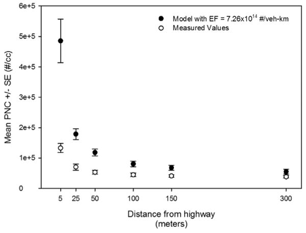
Dispersion model PNC estimates produced with an emission factor of 7.26 × 10¹⁴ #/veh-km. With circles represent the average of the median values observed at all 7 sites along I-10 in El Paso. Data from all sample collection dates were used (Table S1).
Figure 5.

Dispersion model PNC estimates; a) produced with different emission factor values, b) produced with different w* values. Measured values represent data from all sample collection dates were used (Table S1).
Figure 6.

Adjusted PNC estimates produced with an emission factor of 1.82 × 10¹⁴ #/veh-km and compared against averaged measurements per site.
Table 2 lists correlation and fractional bias coefficients for comparisons between measured and estimated values per site. The correlation coefficient was influenced by the higher values observed near the highway, thus fractional bias offered a better assessment of the performance of the model. Since the emission factor was adjusted locally with measured values, it was also pertinent to assess the contribution of the model beyond that of an empirical model. Correspondingly, a regression model that included traffic and distance from highway as predictors was fitted to the data. Based on correlation and fractional bias coefficients the dispersion model seem to produce better PNC estimates than the regression model at all sites except SB (Table 2). The value of adjusting the PNC gradients with localized background estimates produced with the LUR model was determined by adjusting the PNC gradients with a constant background value, which was estimated as the averaged background concentration (2.2 × l04 #/cc) across all sites, and comparing both sets against measured values (Table 2). As suggested by the smaller fractional bias coefficients, the inclusion of the LUR estimated PNCB values improves the performance of the dispersion model at all sites. The fractional error for the LUR-adjusted estimates averaged 6% compared to 40% for estimates adjusted with a constant background value. Overall the model slightly overestimated the measured values (see Fig. 6). The PNC estimates deviated the most from measured values at the CN and CH sites where fractional bias was -13% and 10%, respectively.
Table 2.
| Site | Measurements vs.dispersion Model | Measurements vs. regression Modela | Measurements vs. dispersion Modelb | |||
|---|---|---|---|---|---|---|
|
|
|
|
||||
| R | FB | R | FB | R | FB | |
| CN | 0.90 | ‒13% | 0.87 | ‒52% | 0.83 | ‒25% |
| EX | 0.84 | ‒8% | 0.94 | ‒85% | 0.78 | ‒52% |
| UT | 0.91 | 7% | 0.55 | ‒82% | 0.72 | ‒47% |
| LA | 0.66 | ‒3% | 0.63 | 29% | 0.91 | 77% |
| SB | 0.92 | ‒1% | 0.75 | ‒6% | 0.89 | 35% |
| CH | 0.89 | 10% | 0.94 | ‒4% | 0.98 | 31% |
| TB | 0.84 | 3% | 0.93 | ‒21% | 0.84 | ‒16% |
R = correlation coefficient for analysis between median of measured values and estimated PNC.
FB (%) = fractional bias: .
Model form: 37728+654.2*V*exp(-0.02*x).
PNC adjusted with constant background (2.2 × 10⁴ #/cc).
3.4. Annual average daily PNC estimates
The annual average daily PNC estimates along I10 were predicted using an annual average wind speed (u) of 3.6 m/s, w* = 1.5, h = 1 m, z = 2 m, and EF= 1.63 × l014 #/veh-km for all locations. The only variable inputs across locations were traffic volume and distance. PNC estimates produced with the dispersion model were adjusted by adding PNCB, which was estimated via LUR. The 98 sets of long-term PNC estimates were rasterized into a continuous surface along I10 (Fig 7). The highest and lowest predicted PNC values were 1.3 × l05 #/cc and 9.8 × l03 #/cc, respectively. The average PNC was 2.5 × 10 #/cc (SE 421.0). The highest PNC occurred within highly urbanized areas where traffic volumes on both I10 and arterial roadways are highest. The lowest PNC occurred towards the north and south part of the study area and away from densely urbanized areas. Between the EX and UT sites I10 passes through a small mountainous region where there arterial traffic is low or nonexistent resulting in low LUR estimated PNCB values and consequently lower adjusted-PNC values. The averaged adjusted-PNC5 values between EX and UT was 6.4 × 10⁴ #/cc. Towards the LA site land-use changes sharply and I10 passes through the downtown area where arterial traffic and consequently adjusted-PNC estimates were higher. The sharp PNC variations between the EX-LA sites accurately reflect the local topography and urban land use patterns.
4. Discussion
An atmospheric dispersion model and a LUR model were used to produce a continuous surface of annual PNC estimates within a 1000-m buffer around I10 in El Paso, Texas. The integration of the two models allowed for the PNC variation within the buffer to reflect emissions from traffic both along and away I10. The results from this study along with those from many others clearly suggest that PNC has at least two scales of spatial variation within urban regions (Hoek et al., 2011; Zhu and Hinds, 2005). The first scale can be measured in meters and encompasses the region immediately around highways and major roadways where PNC variation is high. PNC at this scale can be modeled independently for each major roadway using a dispersion model. The second scale encompasses the entire arterial roadway network within an urban region and can be measured in kilometers. The variation of PNC across this scale is a function of multiple variables (e.g., roadway density, traffic volumes, other sources, meteorological conditions). LUR modeling has consistently been shown to adequately capture the variability of multiple air pollutants including PNC, at this scale (Hoek et al., 2011, 2008; Jerrett et al., 2004; Johnson et al., 2010). The analysis of these two scales of variation revealed that in areas of high arterial traffic (e.g., LA, SB, CH) background concentrations can be comparable or higher than near-highway concentrations in less urbanized areas (e.g., CN). Evidently, for purposes of exposure assessment and health studies, the characterization of PNC at these two scales is necessary.
Selecting an emission factor was particularly challenging. Ideally, an emission factor should be obtained locally to adequately account for local meteorological and traffic conditions. Determining an emission factor locally also provides control over the measurement instruments and the particle size range, enabling a more robust model performance evaluation. Several methodologies to determine particle number emission factors have been published and many of them could be feasibly reproduced elsewhere (Keogh et al., 2009; Zhu and Hinds, 2005). Published emission factors have been produced under varying meteorological and traffic conditions, following diverse methodologies, and thus include a wide range of values (Keogh et al., 2009; Zhu and Hinds, 2005). The selection of an emission factor should at least consider the traffic fleet composition, road type, meteorological conditions particularly relative humidity and wind speed, and the particle size range associated with its generation. In the absence of an emission factor a good alternative is to generate a regression model based on local measurements (Patton et al., 2014; Zwack et al., 2011). The advantage of regression models is that they fit measured values and their accuracy is determined by the representativeness of the measured values not by emission inputs (Patton et al., 2014). In this study, the performance of the dispersion model was slightly better than that of an exponential decay (regression) model (see Table 2). However, regression models are highly dependent on the representativeness of the ambient measurements (Patton et al., 2014), which in this case was limited by the short measurement campaigns. Given the promising performance of regression models (Patton et al., 2014; Zwack et al., 2011) and dispersion models (Zhu and Hinds, 2005) for estimating near-highway concentration of ultrafine particles a comprehensive evaluation of these two modeling approaches is necessary. Finally, the characterization of local particle emissions sources in urban environments by combining dispersion modeling and regression analyses of mobile monitoring data is particularly intriguing (Zwack et al., 2011).
This study had several limitations. For instance, wind speed, wind direction, temperature, and relative humidity have all been shown to impact ambient PNC (Olvera et al., 2013; Zhu et al., 2004, 2006). In El Paso, temperature and humidity are highest in July and August, and lowest in December and January (Olvera et al., 2013). The measurement periods captured a wide range of meteorological variation as shown in Tables 1 and S1. However, the impact of high wind speeds (e.g., > 9 m/s) common during spring and that result in lower PNC was not adequately captured (Olvera et al., 2013). Using the dispersion model and local wind speed data for 2012, it was estimated that the difference in averaged PNC would be less than 1% higher when the average wind speed from July through November is used instead of the annual average. The small impact of not including the high wind speed episodes was primarily due to the small frequency of these events. Since we purposely selected measurement periods when the wind was blowing from the highway towards the measurement sites, in terms of wind direction, the impact is expected to be overestimation of PNC. Ideally, longer measurements under all wind conditions would be recommended to ensure long-term conditions are properly captured at every site. Also, we produce symmetric gradients along I10 to estimate long-term PNC that accounted for varying wind directions throughout the year. Although this was a conservative and practical approach, a more appropriate alternative could be to estimate the PNC gradients for multiple wind directions and produce a weighted average at each location using wind direction frequencies (i.e., wind roses) as weights. This approach was not feasible at this time, as it requires long-term wind direction measurements at each site to produce the weights.
Another limitation was the small number of sites used to generate the LUR model. It is well established that for purposes of LUR modeling, ambient measurements should adequately capture the spatial and temporal variation of the pollutant of interest across the modeling region. In this study, we intended to capture the spatial variability of PNC by purposely locating monitoring sites in areas affected by the distinct traffic conditions found across the region. To capture the large temporal variation of PNC in the region, simultaneous measurements conducted for extended periods of time would have been ideal. Unfortunately, simultaneous measurements were not possible due to the availability of a single SMPS instrument. Instead, measurements were conducted during periods selected to capture distinctive traffic and meteorological conditions. For instance, measurements were performed during the summer when traffic demand is lowest, and during the fall and early winter when traffic demand is highest (Olvera et al., 2013). Still, some conditions were not adequately captured, like those during weekends and nighttime hours, when traffic demand is low. Consequently, PNCB might have been overestimated. Based on data collected at a local port of entry, it was estimated that long-term PNC averages produced with data collected only on weekdays would be 14% higher than if produced with data collected throughout the entire week (Olvera et al., 2013).
Finally, the PNC surface shown in Fig. 7 was produced by rasterizing PNC estimated at every point of the Near-Highway Grid. These PNC estimates did produce gradients at each of the 98 locations. However, rasterizing PNC in to a single surface slightly masked some of these gradients, particularly those towards the edges of the region and in areas of high spatial PNC variation (e.g., between EX and UT sites). The rasterized PNC surface was produced with PNC estimated at all points of the near-highway grid (see Fig. 1). The rasterizing process does not account for the highway and thus fails to adequately interpolate the near highway values. Also, towards the edges of the region the rasterizing process masked the PNC gradients away from I10 because PNC5 estimates in these areas were lower than PNC300 in high traffic zones (e.g., downtown). A solution could be to increase the resolution of the grid in areas where the expected spatial variation of PNC is high, such as in areas of complex terrain or sharp change in land-use.
Figure 7.

Long-term PNC surface along Interstate 10 in El Paso, Texas. Surface was produced with PNC estimates produced with the dispersion model and adjusted to local background concentrations (PNCB) estimated with the LUR model at 98 locations along I10.
5. Conclusions
In this study, atmospheric dispersion and LUR models were used in conjunction to estimate PNC within a 1000 m buffer along I10 within El Paso, Texas. The economy and good performance of the two modeling techniques employed in this study, suggest that producing a regional PNC surface to assist in the assessment chronic exposure to ultrafine particles, would be highly feasible in those urban regions across the world were traffic and meteorological data is readily available. The characterization of PNC at regional scales is crucial to the study of UFP exposure and its impacts on human health. Regional surfaces of PNC can help produce detailed exposure assessments that cover the places where people live, work, learn, play, and pray. In this regard, integrating both near-highway and regional models to estimate PNC across an urban region can lead to comprehensive exposure assessments and the advancement of environmental health research.
Supplementary Material
Highlights.
Annual particle number concentrations around a highway were estimated.
Atmospheric dispersion and land use regression models were used.
The emission factor and the background adjustment had an impact on accuracy.
The two models captured the impact of traffic near and away from the highway.
The modeling technique would be feasible in regions where traffic data is available.
Acknowledgments
This project was supported by Award Number 3P20MD002287-05S1 from the National Institute on Minority Health and Health Disparities and the Environmental Protection Agency. The content is solely the responsibility of the authors and does not necessarily represent the official views of the Hispanic Health Disparities Research Center, the National Institute on Minority Health and Health Disparities or the National Institutes of Health, or the Environmental Protection Agency.
Footnotes
Appendix A. Supplemental information: Supplemental information related to this article can be found at http://dx.doi.org/10.1016/j.atmosenv.2014.09.030.
References
- Babyak M. What you see may not be what you get: A brief, nontechnical introduction to overfitting in regression-type models. Psychosom Med. 2004;66:411–421. doi: 10.1097/01.psy.0000127692.23278.a9. [DOI] [PubMed] [Google Scholar]
- Chalupa DC, Morrow PE, Oberdörster G, Utell MJ, Frampton MW. Ultrafine particle deposition in subjects with Asthma. Environ Health Perspect. 2004:1–4. doi: 10.1289/ehp.6851. http://dx.doi.org/10.1289/ehp.6851. [DOI] [PMC free article] [PubMed]
- Daigle C, Chalupa D, Gibb F, Morrow P, Oberdörster G, Utell M, Frampton M. Ultrafine particle deposition in humans during rest and exercise. Inhal Toxicol. 2003;15:539–552. doi: 10.1080/08958370304468. [DOI] [PubMed] [Google Scholar]
- Green S. How many subjects does it take to do a regression analysis? Multivar behav res. 1991;26:499–510. doi: 10.1207/s15327906mbr2603_7. [DOI] [PubMed] [Google Scholar]
- Hoek G, Beelen R, de Hoogh K, Vienneau D, Gulliver J, Fischer P, Briggs D. A review of land-use regression models to assess spatial variation of outdoor air pollution. Atmos Environ. 2008;42:7561–7578. http://dx.doi.org/10.1016/j.atmosenv.2008.05.057. [Google Scholar]
- Hoek G, Beelen R, Kos G, Dijkema M, van der Zee SC, Fischer PH, Brunekreef B. Land use regression model for ultrafine particles in Amsterdam. Environ Sci Technol. 2011;45:622–628. doi: 10.1021/es1023042. http://dx.doi.org/10.1021/es1023042. [DOI] [PubMed] [Google Scholar]
- Jacobson M. Evolution of nanoparticle size and mixing state near the point of emission. Atmos Environ. 2004;38:1839–1850. http://dx.doi.org/10.1016/j.atmosenv.2004.01.014. [Google Scholar]
- Jamriska MM, Morawska LL. A model for determination of motor vehicle emission factors from on-road measurements with a focus on submicrometer particles. Sci Total Environ. 2001;264:241–255. doi: 10.1016/s0048-9697(00)00720-8. http://dx.doi.org/10.1016/S0048-9697(00)00720-8. [DOI] [PubMed] [Google Scholar]
- Jerrett M, Arain A, Kanaroglou P, Beckerman B, Potoglou D, Sahsuvaroglu T, Morrison J, Giovis C. A review and evaluation of intraurban air pollution osure models. J Expo Anal Environ Epidemiol. 2004;15:185–204. doi: 10.1038/sj.jea.7500388. http://dx.doi.org/10.1038/sj.jea.7500388. [DOI] [PubMed] [Google Scholar]
- Johnson M, Isakov V, Touma JS, Mukerjee S, Özkaynak H. Evaluation of land-use regression models used to predict air quality concentrations in an urban area. Atmos Environ. 2010;44:3660–3668. http://dx.doi.org/10.1016/j.atmosenv.2010.06.041. [Google Scholar]
- Keogh DU, Kelly J, Mengersen K, Jayaratne R, Ferreira L, Morawska L. Derivation of motor vehicle tailpipe particle emission factors suitable for modelling urban fleet emissions and air quality assessments. Environ Sci Pollut Res. 2009;17:724–739. doi: 10.1007/s11356-009-0210-9. http://dx.doi.org/10.1007/s11356-009-0210-9. [DOI] [PubMed] [Google Scholar]
- Kumar P, Ketzel M, Vardoulakis S, Pirjola L, Britter R. Dynamics and dispersion modelling of nanoparticles from road traffic in the urban atmospheric environment—a review. J Aerosol Sci. 2011;42:580–603. http://dx.doi.org/10.1016/j.jaerosci.2011.06.001. [Google Scholar]
- Löndahl J, Massling A, Pagels J, Swietlicki E, Vaclavik E, Loft S. Size-resolved respiratory-tract deposition of fine and ultrafine hydrophobic and hygroscopic aerosol particles during rest and exercise. Inhal Toxicol. 2007;19:109–116. doi: 10.1080/08958370601051677. http://dx.doi.org/10.1080/08958370601051677. [DOI] [PubMed] [Google Scholar]
- Morawska L, Ristovski Z, Jayaratne ER, Keogh DU, Ling X. Ambient nano and ultrafine particles from motor vehicle emissions: characteristics, ambient processing and implications on human exposure. Atmos Environ. 2008;42:8113–8138. http://dx.doi.org/10.1016/j.atmosenv.2008.07.050. [Google Scholar]
- Mulaik SA. The curve-fitting problem: an objectivist view. Philos Sci. 2001;68:218–241. [Google Scholar]
- Oberdörster G, Oberdörster E, Oberdörster J. Nanotoxicology: An Emerging Discipline Evolving from Studies of Ultrafine Particles. Environ Health Perspect. 2005;113:823–839. doi: 10.1289/ehp.7339. http://dx.doi.org/10.1289/ehp.7339. [DOI] [PMC free article] [PubMed] [Google Scholar]
- Olvera HA, Garcia M, Li WW, Yang H, Amaya MA, Myers O, Burchiel SW, Berwick M, Pingitore NE., Jr Principal component analysis optimization of a PM2.5 land use regression model with small monitoring network. Sci Total Environ. 2012a;425:27–34. doi: 10.1016/j.scitotenv.2012.02.068. http://dx.doi.org/10.1016/j.scitotenv.2012.02.068. [DOI] [PMC free article] [PubMed] [Google Scholar]
- Olvera HA, Lopez M, Guerrero V, Garcia H, Li WW. Ultrafine particle levels at an international port of entry between the US and Mexico: Exposure implications for users, workers, and neighbors. J Expo Sci Environ Epidemiol. 2013 doi: 10.1038/jes.2012.119. http://dx.doi.org/10.1038/jes.2012.119. [DOI] [PubMed]
- Olvera HA, Perez D, Clague JW, Cheng YS, Li WW, Amaya MA, Burchiel SW, Berwick M, Pingitore NE. The effect of ventilation, age,and asthmatic condition on ultrafine particle deposition in children. Pulm Med. 2012b;2012:1–9. doi: 10.1155/2012/736290. http://dx.doi.org/10.1155/2012/736290. [DOI] [PMC free article] [PubMed] [Google Scholar]
- Perkins JL, Padró-Martínez LT, Durant JL. Particle number emission factors for an urban highway tunnel. Atmos Environ. 2013;74:326–337. doi: 10.1016/j.atmosenv.2013.03.046. http://dx.doi.org/10.1016/j.atmosenv.2013.03.046. [DOI] [PMC free article] [PubMed] [Google Scholar]
- Rivera M, Basagaña X, Aguilera I, Agis D, Bouso L, Foraster M, Medina-Ramón M, Pey J, Künzli N, Hoek G. Spatial distribution of ultrafine particles in urban settings: A land use regression model. Atmos Environ. 2012;54:657–666. http://dx.doi.org/10.1016/j.atmosenv.2012.01.058. [Google Scholar]
- Sharan M, Singh MP, Yadav AK. Mathematical model for atmospheric dispersion in low winds with eddy diffusivities as linear functions of downwind distance. Atmos Environ. 1996a;30:1137–1145. [Google Scholar]
- Sharan M, Yadav AK, Singh MP, Agarwal P, Nigam S. A mathematical model for the dispersion of air pollutants in low wind conditions. Atmos Environ. 1996b;30:1209–1220. [Google Scholar]
- Stewart JC, Chalupa DC, Devlin RB, Frasier LM, Huang LS, Little EL, Lee SM, Phipps RP, Pietropaoli AP, Taubman MB, Utell MJ, Frampton MW. Vascular Effects of Ultrafine Particles in Persons with Type 2 Diabetes. Environ Health Perspect. 2010;118:1692–1698. doi: 10.1289/ehp.1002237. http://dx.doi.org/10.1289/ehp.1002237. [DOI] [PMC free article] [PubMed] [Google Scholar]
- Weichenthal S. Selected physiological effects of ultrafine particles in acute cardiovascular morbidity. Environ Res. 2012;115:26–36. doi: 10.1016/j.envres.2012.03.001. http://dx.doi.org/10.1016/j.envres.2012.03.001. [DOI] [PubMed] [Google Scholar]
- Zhang K, Wexler A, Niemeier D, Zhu Y, Hinds W, Sioutas C. Evolution of particle number distribution near roadways. Part III: traffic analysis and on-road size resolved particulate emission factors. Atmos Environ. 2005;39:4155–4166. [Google Scholar]
- Zhang KM, Wexler AS. Evolution of particle number distribution near roadways—Part I: analysis of aerosol dynamics and its implications for engine emission measurement. Atmos Environ. 2004;38:6643–6653. http://dx.doi.org/10.1016/j.atmosenv.2004.06.043. [Google Scholar]
- Zhu Y, Hinds W, Kim S, Shen S, Sioutas C. Study of ultrafine particles near a major highway with heavy-duty diesel traffic. Atmos Environ. 2002;36:4323–4335. [Google Scholar]
- Zhu Y, Hinds W, Shen S. Seasonal trends of concentration and size distribution of ultrafine particles near major highways in Los Angeles. Special Issue of Aerosol Science and Technology in Findings from the Fine Particulate Matter Supersites Program. Aerosol Sci Technol. 2004;38(S1):5–13. http://dx.doi.org/10.1080/02786820390229156. [Google Scholar]
- Zhu Y, Hinds WC. Predicting particle number concentrations near a highway based on vertical concentration profile. Atmos Environ. 2005;39:1557–1566. http://dx.doi.org/10.1016/j.atmosenv.2004.11.015. [Google Scholar]
- Zhu Y, Kuhn T, Mayo P, Hinds WC. Comparison of daytime and nighttime concentration profiles and size distributions of ultrafine particles near a major highway. Environ Sci Technol. 2006;40:2531–2536. doi: 10.1021/es0516514. http://dx.doi.org/10.1021/es0516514. [DOI] [PubMed] [Google Scholar]
Associated Data
This section collects any data citations, data availability statements, or supplementary materials included in this article.