Population Growth and Its Spatial Distribution as Factors in the Deforestation of Nang Rong, Thailand

Abstract

Frontiers constitute a major source of global land cover change hot spots, with forests and grass lands being converted into agricultural uses. As such, frontiers provide an opportunity to see how people manipulate the land and their lives in the context of social, cultural and environmental constraints. This paper examines frontier settlement and land cover change in Nang Rong district, Northeast Thailand for the last half century. It uses a Cellular Automata (CA) model to explore the land cover consequences of alternative patterns of settlement in a setting where people establish dwelling units in nucleated villages and work agricultural plots that surround villages. Forested land around the center of a village is converted into agricultural uses in an inverse relationship to the distance from the village center, but frequently modified by biophysical conditions. Land at the center of the village may be reforested after the village is established as a source of shade as well as fruit and other products. Model variation in land cover change is more sensitive to the spatial reach of village households than their temporal reach, suggesting the important role that technology plays in how villagers travel to their fields (walking versus motorized transit).

INTRODUCTION

Frontier settlement and the rapid conversion of forests to agricultural uses is one of the more visually dramatic examples of the connection between population and the environment. Over the past half century, the expansion of human settlement has precipitated deforestation in many parts of the world. These changes in land cover have had an impact globally (NRC, 2001), as well as locally. While it is obvious that the movement of settlers into a frontier area is responsible for land cover change at a broad scale, the patterning of effects at finer scales is not as well understood and depends on setting. Any attempt to guide settlement processes should be informed by a detailed understanding of the timing, nature, and areal extent of their impact.

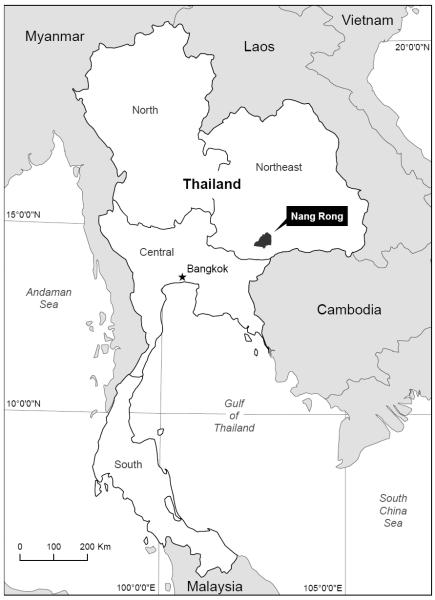
This paper examines frontier settlement and land cover change over the last half century in Nang Rong, a district in Northeast Thailand. Nang Rong occupies approximately 1300 km² in Northeast Thailand (Map 1). A century ago, the district was mostly forested. Since that time, large numbers of settlers moved into the region, especially in the latter half of the 20^th century, leading to the extensification of agriculture and associated deforestation. Now, in the lower elevations, there is paddy land, used primarily for rain-fed rice cultivation, and in the higher elevations, open-canopy forest and dry field crops (Fukui, 1993). The environmental setting is one of marginality: relatively low soil fertility, unpredictable precipitation, insufficient drainage, and generally speaking, a limited natural resource base. We use unique data on the history of village settlement in Nang Rong to describe an initial effect on the conversion of forest into agricultural uses as settlers move into the region followed by a re-creation of forest in village centers once dwelling units are built.

Map 1.

Location of Nang Rong.

More specifically, this paper uses a Cellular Automata (CA) model to explore patterns of settlement between 1954 and 2000, and their repercussions for land cover change. It does so within the framework of complexity theory (see Manson (2001) and Parker et al. (2003) for reviews). CA models do not describe a complex system with complex equations, but allow complexity to emerge from interactions of basic building blocks that follow simple rules (Messina and Walsh 2005), in our case, rules about the relationships between land use/land cover and the changing characteristics and relative locations of pixels. The next section presents a dynamic theoretical model of settlement and land use change adapted to the Nang Rong setting. Then, the CA model is introduced and issues involved in its assessment reviewed. We then describe the village administrative history data and explain how we use them to describe settlement processes. We draw on aerial photos and satellite data to do likewise for patterns of land cover. The paper then turns to the results of the CA model simulations, interpreting them in terms of the history of Nang Rong, hypotheses about village settlement, and assumptions of the CA model. The conclusion takes stock and sets out logical next steps in model development.

A DYNAMIC MODEL OF SETTLEMENT AND LAND USE CHANGE

An understanding of the impact of population growth on land use and land cover change in a frontier area requires a dynamic perspective that focuses on the spatial distribution of settlement, incorporates both biophysical and social aspects of the broader environment, and flexibly incorporates endogeneities and feedbacks, especially those relevant to continuing in-migration into the area. It also requires sensitivity to the specific opportunities and constraints represented in a setting. Our theoretical approach to settlement and land use change, while general, adapts to the case at hand, Nang Rong, Thailand. We begin with a discussion of the particulars and then embed the model into a more general treatment of complexity theory. The goal of complexity theory is to understand how simple, fundamental processes combine to produce complex holistic systems (Luhman, 1985, Gell-Mann, 1994). Such systems not only evolve through time, but their past is co-responsible for its present behavior (Cilliers, 1998). The feedbacks and nonlinearities that are fundamental to complex systems are clearly evident in the model of settlement and land use/land cover change developed here.

Nang Rong has a long history, extending back several millennia (Fukui, 1993). Certainly, it was not virgin territory in the middle of the 20^th century. It was, however, sparsely populated then, considering the potential of the land to support a growing population given available technology. Settlers from Central Thailand and other parts of the Northeast moved in to Nang Rong over the next several decades (Riethmuller et al., 1984; Phongphit and Hewison, 2001). Dramatic declines in mortality¹ paired with continued high levels of fertility further contributed to population growth. Expansion of agricultural lands continued and may have even accelerated through most of the 1970s, but after 1980, there was little expansion potential left (Siamwalla, 1995). The period covered in this paper, from 1954 to 2000, encompasses a major transition in population and land cover in the district.

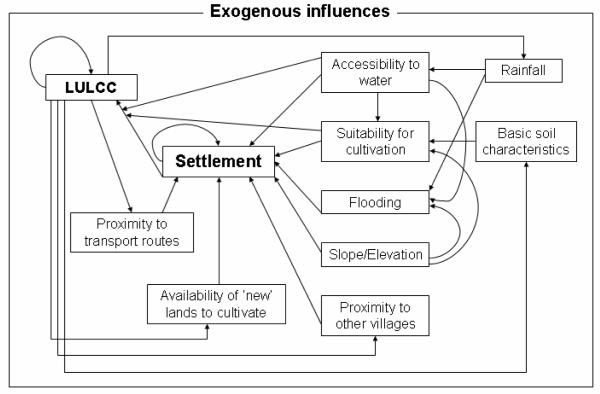
Given the availability of new lands to cultivate in a frontier area, the timing, spatial patterning, and land use consequences of settlement will be affected by biophysical, economic, and social factors operating at several levels. Relevant biophysical factors in Nang Rong are characteristics of the land (slope, elevation, vulnerability to flooding, soil characteristics, and suitability for cultivation), and accessibility to water. Social and economic factors include the sociospatial organization of villages, their size, proximity to other villages, and proximity to transport routes as well as land tenure arrangements, market conditions, and government policies (or the absence thereof). Figure 1 shows our theoretical approach to settlement and land use change in Nang Rong. The model shown in Figure 1 is dynamic, with feedbacks, where the strength of effects depends on the larger social and economic context, which can change over time.

Fig. 1.

Village Settlement Patterns

Consider a subsistence economy based on rain-fed paddy rice cultivation with social and political structures organized around nucleated villages. This was the situation in Nang Rong in 1950. New settlers would have been looking for the best available land for paddy rice cultivation in combination with access to drinking water and a nearby place where houses could be built and safely maintained. Basic soil characteristics, relative elevation, slope, and accessibility to water are the main biophysical characteristics that determine suitability for rice cultivation in this context (Phongphit and Hewison, 2001). Swampy low-lying ground around rivers is particularly good for this purpose (Riethmuller et al., 1984:154). Village residents most likely would want to live close to their fields (farm implements had to be carried back and forth to the village, as did the rice when it was harvested); close to a water source for drinking water for themselves and their animals (Phongphit and Hewison, 2001); and ideally, on a small hill or rise rather than in a lowlying area (Riethmuller et al., 1984). Indeed, security (safety in numbers), power (locally), and return to scale are all enhanced by a clustered residential pattern, with dwelling units grouped, surrounded by agricultural lands (Phongphit and Hewison, 2001; Riethmuller et al., 1984). Settlement is also affected by proximity to other villages and to transportation routes. As we have shown elsewhere (Entwisle et al., forthcoming), in this setting, people prefer to settle relatively close to already established villages to take advantage of potential economies of scale and infrastructure that might have already been developed (e.g., roads, temples) as well as for sociability and potential help in a time of need (a crude form of insurance).

After a new settlement is established, land cover around the settlement changes. A village cluster would be created composed of houses, vegetable gardens, and public areas. Connector paths and roads would be built linking the settlement to other villages and to a main road, if one exists. Villagers first farm land that is closest, but when that land is already farmed, they claim land farther away. We hypothesize that land around the village cluster would be converted to cultivation in a pattern radiating out from the village but influenced by biophysical characteristics such as topography, the spatial distribution of soils, presence of streams and rivers, and the like. These changes in land use would affect subsequent settlement, both new settlement (the creation of a new village nearby) and the expansion of existing settlement. The circular arrow attached to settlement in Figure 1 indicates that once a new village is established, it may grow for many of the same reasons that people initially settled there.

In Nang Rong, once villages reach a certain size, they are subdivided administratively, so the expansion of village settlement coincides with a proliferation of villages. Indeed, as we show below, the number of administrative villages increased dramatically over the period of interest. The location of new villages reflects the spatial distribution of population growth.

Generally speaking, settlers increasingly occupy frontier areas until a threshold is reached, whereby comparative advantages are lost and opportunities elsewhere are better. Absent shifts in the larger social, economic, cultural, or biophysical environment, the frontier closes. In the case of Nang Rong, two exogenous changes occurred that affected relationships and feedbacks within the model: the extension of the national highway system and the emergence of an international market for cassava.

In Thailand, in the 1950s and 1960s, major investments were made in roads (Ingram, 1971; Siamwalla, 1995; VanLandingham and Hirschman, 2001). By 1984, Thailand had one of the most developed road networks in Southeast Asia (Riethmuller et al., 1984:126). The expansion of the road network radically increased the accessibility of the Northeast, tying the region to world markets through Bangkok and somewhat later, the Eastern seaboard, and also facilitating the movement of settlers within the region (Ingram, 1971; VanLandingham and Hirschman, 2001). Nang Rong is located along a major highway, completed in the late 1960s, connecting Nang Rong to markets in Korat (a regional city) and ultimately Bangkok. Korat was a major center for the processing of cassava, a new crop at that time. The road also facilitated the movement of heavy tractors into the district, especially in the southwest, to assist with the preparation of plots for upland crop cultivation. The highway changed the proximity of villages to major routes of transportation, also changing the effect of settlement on land use.

The emergence of an international market for cassava also had an effect on relationships in the model. Demand for this crop originated in European Economic Community (EEC) countries, where it is used as a high-calorie animal-feed supplement. The timing of the expansion of demand for cassava was influenced by two factors. One was an increase in the demand in Europe related to an increase in the demand for livestock more generally. As a supplement for feed, cassava was valued for its high starch content. Germany and The Netherlands, in particular, sought a substitute for high-priced European cereals and found it in Thai cassava. The other factor was the availability of cheap American soy waste with which cassava was mixed, and which came on the European market beginning in 1964 (Riethmuller et al., 1984:133; Siamwalla, 1995). The boom in demand for cassava lasted until 1982, when, in response to EEC demands, a quota was placed on cassava exports (Riethmuller et al., 1984:138; Synder, 1993:4), although not always enforced. Note that cassava is grown for export; it is almost never incorporated into the diet of the average Thai.

As agriculture shifts from subsistence to commercial, proximity to roads would increase in importance. Land not suitable for paddy rice cultivation might acquire value as sites for cassava cultivation. The highway was under construction and completed at the same time as a market for Thai cassava appeared in the EEC in the 1960s. These were watershed events, with the potential to redefine the frontier, making further settlement possible. Moreover, land tenure arrangements encouraged farmers to strategize around short-term profit without regard to the future consequences such as soil exhaustion (Riethmuller et al., 1984:168). Cassava cultivation degrades the soil.² Formally, any land not occupied was government land, but households considered it available for their use (Ingram, 1971; VanLandingham and Hirschman, 2001). Informal tenure arrangements were such that households could claim land and use it. Rights to government land were generally not enforced.

To fully examine the relationships shown in Figure 1 one would need a) deep historical data on the demography of villages and households to track population movements as well as the formation and growth of villages and b) an associated time-series of aerial photographs and satellite images to track land cover change over a fifty year period. Such data are not available for Nang Rong, and indeed only rarely for any frontier (Entwisle and Stern, 2005). Further, because of feedbacks in the model, unless special steps are taken, statistical tests of relationships within it are likely compromised. Regression analysis is typically based on an assumption of zero covariance between the residual or error of the regression equation, and the predictor or independent variables. This assumption is difficult to maintain in a model with feedbacks. Although it is possible to incorporate the feedbacks into a multi-equation statistical model, statistical identification remains a challenge given a dynamically interrelated system such as that depicted in Figure 1. We instead use a simulation approach: cellular automata (CA) modeling.

Within the context of the CA model, described in the next section, we explore the implications of village settlement for trends and patterns of land cover. Of principal interest are two hypotheses about the impact of villages on land cover change over the past half century. First, when a new village is established, we hypothesize that land will be converted from forest to agricultural use, either rice or cassava, depending on biophysical conditions, in inverse relationship to distance from the village center. We further hypothesize that the more time that has passed since the village was established, the greater this effect will be. We label this a “primary effect” of village settlement. The second hypothesis concerns the regeneration of forest cover, which we label a “secondary effect.” When a new village is established, a village cluster is created composed of houses, vegetable gardens, and public areas. Once houses are built, trees are planted in and around the village for shade and as sources of fruit and other products. Some of these trees grow very quickly, e.g., banana trees, whereas others take longer. Over time, the foliage from these trees obscures the roofs of the houses and increasingly, the view from space registers as forest cover rather than some other land cover. Thus, we hypothesize that after a lag, forest cover will begin to appear in the center of the village. Tree growth in the center of villages is, of course, quite different in its composition and use from the forest that originally grew there. Nevertheless, both count as forest cover and need to be taken into account in interpreting the changes that occurred. We use the CA model to explore the consequences of village settlement, especially the timing of effects, for landscape composition.

Complexity theory provides an overarching framework for the entire project. Complexity theory holds that feedbacks and nonlinearities are essential components of systems (Matthews et al., 1999, Manson, 2001), including and perhaps especially coupled human-natural systems. Feedbacks are clearly central to the model of village settlement and land use/land cover change described above (see Figure 1). Interactions between human and natural factors are pervasive, e.g., between accessibility to water and village settlement, as are nonlinearities in the effects of settlement on the use of surrounding lands. Complexity theory conceives the world as consisting of self-organized systems, either reproducing their state (a stable state) through negative feedbacks with their environment, or moving along trajectories from one state to another as a result of positive feedbacks. Land use/land cover dynamics in Nang Rong fit this description. Dynamics emerging from local nonlinear feedbacks can constrain the evolving patterns or create emergence of new landscape structures that create additional feedbacks on subsequent activities. The nonequilibrium functioning of systems is a foundation for the argument that ecosystems exhibit emergence (Holland, 1998) or self-organization (Bak, 1998). We now turn to the operationalization of these ideas.

SIMULATING EFFECTS OF VILLAGE SETTLEMENT

To explore the contribution of village settlement to deforestation and the extensification of agriculture in Nang Rong, we constructed a Cellular Automata (CA) model that incorporates hypotheses about the timing and spatial patterning of effects related to the establishment of administrative villages as well as hypotheses concerning terrain settings, geomorphic conditions, distance to water, topographic relative moisture patterns, and soil suitability scores. Explanation is our goal, not prediction (Brown et al., 2005). CA approaches have been used to investigate land cover change in a variety of settings, both urban (e.g., Batty et al., 1999; Webster and Wu, 1999; White and Engelen, 1993; White et al., 1997) and rural (e.g., Mas et al., 2004; Messina and Walsh, 2001; Silveira et al., 2002; Walsh et al., 2006). Our approach is distinctive in its incorporation of population growth and spatial distribution on an annual basis over almost fifty years.

A CA is a spatially explicit dynamic model that describes the states and changes in the states of a fixed set of cells. In the CA model we develop for Nang Rong, the units of observation are 30 square meter cells (pixels). Modeled cells can be in one of three discrete states: rice, cassava, or forest. In our model, the state of a cell depends on its previous state, the state of its neighbors, and on nonlinear functions of slope angle, landform morphology, distance to water, soil moisture, land quality characteristics, and distance to the nearest village. Land forms, waterways, and soil characteristics are included as influences on land cover change, but they are not allowed to change over the period of interest – consistent with our understanding of the history of Nang Rong. Distance to the nearest village does change as the district becomes increasingly more settled. The rules of the cellular automaton replicate transition functions, emergence occurs in generated systems, and patterns may or may not be persistent with changing components.

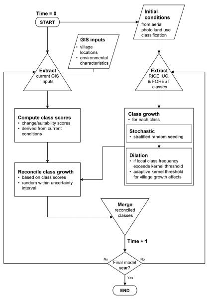
Figure 2 is a generalized schematic of how our CA model operates. The model iterates on annual time steps. At the beginning of each iteration, individual land cover types are extracted from the model output from the previous year. Village locations are updated at each iteration, corresponding to actual settlement patterns. Scores for each class–forest, rice, cassava–are developed based on nonlinear functions of elevation, slope, proximity to a waterway, and proximity to an administrative village. Neighborhood associations within a 3 × 3 cell kernel are used to assess the propensity of focal cells to transition to alternate land cover types depending on the frequencies of these types and change scores occurring within the kernel. Kernel rules change when passing over village centers, boosting the power of village settlement to affect land cover change. A stochastic process is simulated by defining a small number of cells that are randomly seeded as new cells of that class. This random seeding, combined with neighborhood associations that work out over iterations of the model, is how we capture the introduction and spread of upland crops.³ Following each model iteration, land cover classes are recombined based on their likelihood of change to an alternate class using a scaled model input of scores derived from each class. If these differences exceed a defined decision threshold, output class possibilities are randomly selected to represent an “uncertainty interval” in household decision-making and its implications for land cover change. A more complete description of the CA model is in the appendix.

Fig. 2.

A schematic of the CA model.

Spatially-explicit dynamic modeling approaches, such as CA, are well-suited to the exploration of complexity and the explanation of how landscape patterns form and evolve through interactions with heterogeneous places and actors. The complex nature of systems emerges from non-linear relationships due to interactions involving feedbacks occurring at one or more lower levels within the system (Cilliers, 1998; Malanson, 1999; Crawford et al., in press). In the case of frontier settlement, in Nang Rong specifically but also more generally, feedbacks are fundamental as the opportunities awaiting new settlers depend on how previous settlers capitalized on the opportunities that awaited them, thus creating path dependency. In the CA model for Nang Rong, land cover at any point in time depends on what it was in the previous time point as well as the changing number and pattern of villages on the landscape.

PROCESS AND UNCERTAINTY

Fundamental to assessing model performance is determining the general goals of the modeling activity - prediction or explanation (Brown et al., 2005). If prediction is the intent, then the ability of the model to replicate some measure of reality may be an appropriate evaluation metric. In such cases, a satellite image may be retained from an assembled time-series so that the model outcomes of land cover predictions over time can be compared to the reference data to judge the ability of the model to reproduce acceptable estimates of landscape composition and spatial structure. If the goal of the modeling exercise is explanation, then the outcomes of the model need to be assessed relative to the theoretical and empirical understanding of pattern-process relations (Malanson, 1999), and the nature of the rules used to develop the spatial simulations (Messina and Walsh, 2005). In this instance, sensitivity testing as well as comparisons with reference data are in order. Our goal is explanation.

The CA model facilitates the development of candidate explanations for specific landscape patterns, examining factors that can alter trajectories of landscape change resulting in possible shifts in the composition and spatial structure of the landscape. In developing CA transition or growth rules to assess land cover dynamics, there is the temptation to over-parameterize the model and hence “over fit,” rendering the model deterministic in nature. This is true whatever the focus of the modeling is. When models are “over fit,” key elements of complex systems such as emergent behavior, self-organization, and complex adaptive behavior may be severely constrained and not visible. In the case of the model presented here, as explained earlier, we have deliberately not incorporated all of the factors hypothesized to influence land cover change in Nang Rong.

Calibration of the model is commonly accomplished by comparing the model outcomes to a series of classified satellite images, and fine-tuning the rules and relationships to generate improved model fit (Deadman et al., 2004). The danger is that this approach trades fit for generality and applicability. The fine-tuned model may reproduce more or less exactly what happened, but unless the future is a straightforward extrapolation of the past, projections based on it are likely to be wrong. In the initial construction of our CA model, we examined simulated landscapes against a set of expectations partly based on satellite imagery. The CA was calibrated based on gross departures from expectations (e.g., varying the kernel window to better capture “neighborhood effects”). However, no calibration was done to adjust the timing of settlement effects, or their extent, in the basic model. We did not know the outcome of the scenario assessment or sensitivity testing reported in the next section until we did it.

Error and uncertainty in spatial simulation models generated through CA models is an unsettled and contested issue in the research literature (e.g., Bian, 1997; Messina and Walsh, 2005; Rindfuss et al., 2004). For instance, validating model outcomes for historical, contemporary, and future periods; testing “what if” scenarios of land use change; assessing pattern vs. process accuracy of models; and examining the path dependence and independence of models are among some of the more important issues that are yet to be fully addressed. Most common is the characterization of model runs relative to observed landscape conditions, often measured through a satellite image time-series. Summary correlations have been used to describe the nature of compositional agreement between the model and the satellite images, and ecological pattern metrics are used to describe and compare the spatial structure of land cover types.

Here we assess the outputs of our scenarios and model simulations by comparing them to satellite observations. In essence, we are concerned about our ability to replicate observed spatial and compositional patterns, and hence trend lines and pattern metrics are used to assess the certainty or plausibility of our model outcomes relative to observations of reality. We also assess the sensitivity of the simulations to assumptions about the spatial extent of the village settlement effect. Other approaches to assess model performance are under development (Manson, 2003) including the study of pattern invariant areas in simulations (Brown et al., 2005), and emergent patterns and the creation of development fronts through the actions of individuals or some set of base actors on the landscape (Malanson et al., 2006). There are many approaches being used to consider model performance, although there is no unifying protocol yet established. The characterization of prediction vs. explanation is a useful dichotomy to begin to assess theory and practice as applied to spatial simulation outcomes.

DATA ON SETTLEMENT AND LAND COVER CHANGE

Our focus is the effects of village settlement history on land cover dynamics, specifically growth in the number and spatial distribution of villages. In Nang Rong, villages are made up of relatively small numbers of households that farm lands surrounding the cluster of dwelling units. When clusters reach a certain size–typically 100 households, although it varies–an administrative village is created. When the number of households grows too large–typically over 200, although again, it varies–the village is divided administratively into two or more villages. Growth in the number of administrative villages and their locations thus reflects growth in the number of households and their distribution on the landscape. From the standpoint of impact on land use and the environment, the number of households appears to be as or more important than the number of persons (Brondizio et al., 2002; Entwisle et al., 2005; Liu et al., 2003; Liu et al., 1999; McCracken et al., 1999; for an exception, see Foster et al., 2003).

Data to describe the historical pattern of village settlement comes from the 2000 Nang Rong Community Survey, which included all villages within the 1984 boundaries of the district. We use information collected in the community survey on the year that the first village headman was appointed to track the history of villages. The year that the village first had a headman identifies a date of “birth” for the administrative village. The 346 villages in the 2000 survey reported establishment dates ranging from the 17th century to the year of the survey. Of the 346 villages existing in 2000, 267 (77 percent) were established on or after 1950. The number of villages tripled between 1950 and 2000. Some of these villages were brand new, that is, dwelling units were built and settlers moved into an area that had not previously been occupied, whereas others were formed as the result of administrative divisions (Entwisle et al., forthcoming).

Clearly, the consequences for land cover change due to expanded village settlement will depend on where the new villages are located. As part of the 2000 Community Survey, geographic point locations were collected for all 346 administrative villages. Generally, a cross-roads in the village cluster served as the central point for the village. If there was not a cross-roads, the residence of the village headman was selected as the central point. The point locations and establishment dates for the administrative villages were incorporated as additional coverages into an already existing Geographic Information System (GIS) and were used as inputs into the simulations of land cover described below. More direct information about population growth would be desirable, of course, but is only available for a sample of villages over a more limited time series (starting in 1984, after many of the land use and land cover changes of chief interest have already occurred). It is nevertheless worth noting a close relationship between number of households and the creation of new administrative villages in the restricted data set, validating our general approach.

The starting point for the simulations was a set of aerial photos for 1954 (1:40,000 scale). These were scanned, registered, rectified and mosaicked together to create a single unified picture for the entire district. Based on visual inspection, it was clear that in 1954, not including waterways or the town of Nang Rong (located in the middle of the district), land cover could be classified largely as either forest or rice. Map 2 shows the 1954 image classified into these categories, with the villages existing at that time overlaid on top. Forest covered a little over half of the landscape (54.8%). Most of the remainder was in rice (41.5%). Other land in the image was occupied by ponds, rivers, and streams and also by what would become Nang Rong town, in the center of the district, which we mask out. Upland agriculture was not yet a factor at this time.

Map 2.

Land use and land cover in 1954: Classified aerial photo.

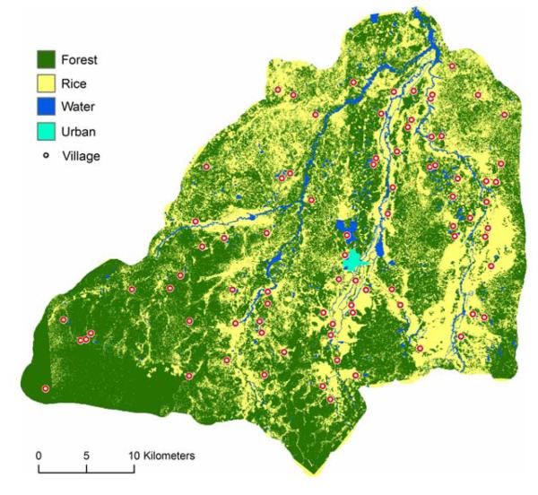
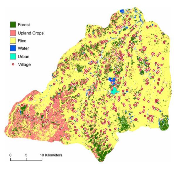
The picture in 2000 contrasts dramatically with that in 1954. Map 3 shows a Landsat Thematic Mapper (TM) satellite image for December 1999 classified in terms of forest, rice, and upland agriculture (primarily cassava but also including sugar cane, maize, and kenaf).⁴ Administrative villages existing in 2000 are overlaid on the classified satellite image. The expansion of settlement into the south and west of the district, as well as the densification of settlement overall, is clearly evident, as are marked changes in land cover. Whereas the district was heavily forested in 1954, most of the forest cover had disappeared by 2000. The area devoted to paddy rice cultivation expanded throughout most of the lowlying areas, and the area devoted to cassava and field crops expanded throughout most of the uplands. Between 1954 and 2000, the percent of land in forest cover declined from 54.8% to 13.3%, while the percent in rice increased from 41.5% to 62.6%. The percent in cassava increased from 0 to 16.7%. Forest remains in the steeper elevations, along riparian corridors, and in small patches through the district. The goal of the simulations is to account for these changes in land cover, with particular reference to potential village settlement effects.

Map 3.

Land use and land cover in 1999: Classified TM image.

SIMULATION RESULTS

We use the CA model to explore the implications of two hypotheses about the timing and nature of the effects of village settlement patterns on land cover change between 1954 and 2000. To briefly review, when a new village is established administratively, we hypothesize that land will be converted from forest to agricultural uses in a pattern radiating out from the village center and shaped by the biophysical environment and proximity to other villages. This is the primary effect of village settlement. Once a village cluster is created, and dwelling units built, after a lag, tree cover will begin to re-appear in the village center as a source of shade as well as fruit and other products. This is the secondary effect of village settlement. Of key interest are the consequences of the timing of primary and secondary effects.

We consider four scenarios, each of which is a different combination of primary and secondary effects. Scenarios A and B model primary effects only, the contrast between them designed to shed light on the timing of these effects. In Scenario A, the effect of village settlement on land cover begins when the village is formally established. The CA uses a contemporaneous village coverage for each iteration of the model (e.g., the coverage from 1970 in predicting land cover for 1971). Scenario B acknowledges the presence of people on the landscape before their numbers are sufficient for administrative recognition. The effect of village settlement on land cover begins ten years prior to formal establishment in this scenario. The CA uses a village coverage from ten years in the future for each iteration of the model (e.g., the coverage in 1980 in predicting land cover for 1971). Because our data end in 2000, there is a question about how to handle the impact of village settlement on land cover change in the 1990s in Scenario B. For the sake of simplicity, we assume no further village growth; clearly, this is an assumption that can be modified in future work.

In contrast to the first two scenarios, which feature primary effects of village settlement, Scenarios C and D also include a secondary effect, each of which is lagged ten years after the onset of the primary effect. In Scenario C, the primary effect of village settlement on land cover change begins when the village is formally established (e.g., the 1970 village coverage in predicting land cover for 1971). This is the same timing as in Scenario A. In contrast to scenario A, however, in Scenario C, there is a secondary effect that begins ten years after that (e.g., the 1960 coverage in predicting an additional effect on land cover for 1971). The contrast between Scenarios A and C sheds light on the importance of the secondary effect. There is a similar contrast between the Scenarios B and D.

We explore the implications of each scenario for landscape composition. At the beginning of each model iteration, we incorporate the village coverage for that year, or for an alternative year, depending on the goals of the simulation. The classified 1954 image described above is used to set initial conditions. We mask out the area occupied by Nang Rong town, as urbanization is not the focus of our modeling effort. We allow the model to run for 46 years to simulate the 1954-2000 interval. We track trends in the percent of the land cover in forest, rice, and upland agriculture between 1954 and 2000, comparing the results to satellite image classifications for dates between 1973 and 1999.

Our primary focus is the timing of village settlement effects, i.e., temporal extent, but we also assess the sensitivity of our model runs to assumptions about their spatial extent. In the main analyses, we limit the primary effect to 1.5 kilometers, and the secondary effect to 0.25 kilometers. The 1.5 kilometer radius for the primary settlement effect roughly corresponds to the distance farmers might be willing to walk, the usual mode of transportation during the period, under a hot equatorial sun carrying their agricultural implements. The 0.25 kilometer radius for the secondary effect corresponds to the likely size of the dwelling unit cluster. The sensitivity assessment allows the primary effect to range from 1.0 to 2.0 kilometers and the secondary effect from 0.25 to 0.50 kilometers.

Simulated trends in land cover

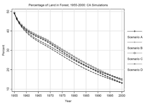
We turn first to Figure 3, which shows simulated trends in forest cover. All of the simulations begin with the 1954 image. In 1954, 54.8% of the landscape was in forest. In 2000, the simulated fraction ranges narrowly between 13.1% and 15.3%, depending on the combination and timing of primary and secondary settlement effects represented in each scenario. The trend slopes strongly downward for all of the simulations, although there is some minor variation around this theme. Scenarios A and C (which both assume a contemporaneous primary settlement effect), and Scenarios B and D (which assume a primary effect that leads the formal establishment of an administrative village), emerge as separate groupings in the 1960s and 1970s. This indicates some impact for the timing of the primary settlement effect in the first half of the period covered, given the other assumptions of the CA model. The timing of the primary effect is the same in Scenarios A and C (contemporaneous with the formal establishment of a village), and it differs from that in Scenarios B and D (which leads by ten years). The pattern of difference in the simulated trends changes during the 1980s such that by the early 1990s, Scenarios A and B (which have no secondary village settlement effect), and Scenarios C and D (which do) emerge as separate groupings. Whether or not there is a secondary settlement effect makes more of a difference than the timing of the primary effect for the fraction of land in forest later in the period. The differences across the scenarios are not large, but the reorganization of differences over the period shows the importance of considering the entire period in an assessment of the scenarios, not just focusing on the endpoint.

Fig. 3.

Percentage of land in forest, 1955-2000: CA simulations.

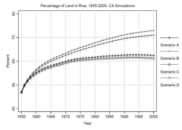
Differences across scenarios are more dramatic for trends in rice and upland crops than for forest. Figure 4 shows the trends for rice. There is a substantial difference between Scenarios A and C (which have a contemporaneous primary village settlement effect) and Scenarios B and D (where the primary effect leads by ten years) that emerges early in the period and increases through time. A ten year difference in the timing of the primary effect of village settlement translates roughly into a ten percentage point difference in the amount of land in rice a half century later. In 2000, the simulated percent in rice ranges between 62 and 61 percent for Scenarios A and C, respectively, and between 73 and 71 percent for Scenarios B and D. Relative to the primary effect, the secondary effect of village settlement is less pronounced. The percent of land in rice is one or two percentage points lower in Scenarios C and D, which include a secondary effect, than in Scenarios A and B, which do not.

Fig. 4.

Percentage of land in rice, 1955-2000: CA simulations.

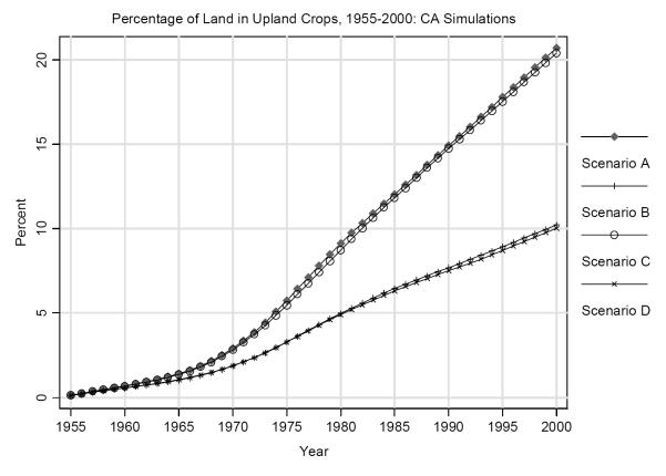
Figure 5 shows the simulated trends for cassava and other upland crops. No limits were put on the expansion of upland crops (cf. Walsh et al., 2006). Trends associated with Scenarios A and C and with Scenarios B and D diverge through the period. In the simulations, as was the case for rice, a ten year difference in the timing of the primary settlement effect translates into a ten percentage point difference in land devoted to cassava and other upland crops by the end of the period. The simulated fraction of land in cassava and other upland crops for 2000 is 21 and 20 percent for Scenarios A and C, respectively, and 10 percent for Scenarios B and D. In contrast to the patterns for rice, the secondary settlement effect has no impact on the simulated fraction of land in upland crops. The trend lines for the four scenarios are virtually identical.

Fig. 5.

Percentage of land in upland crops, 1955-2000: CA simulations.

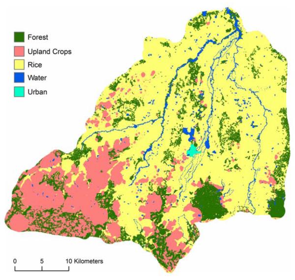
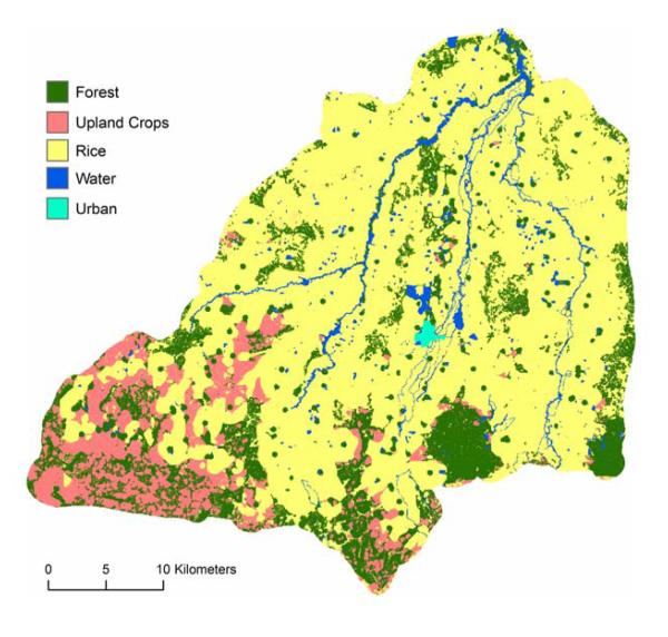
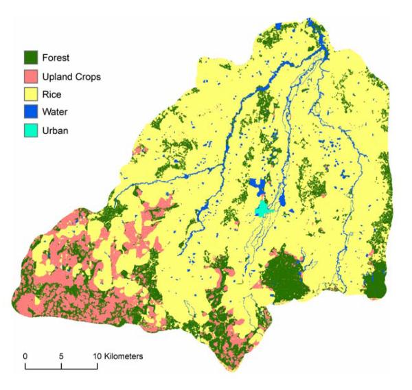
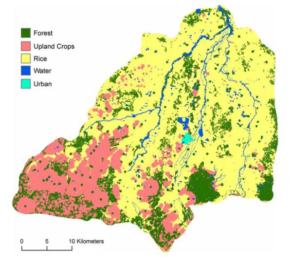
Maps 4-7 present the simulated land cover for the district in 2000 based on each of the scenarios (A-D, respectively). The contrast between Maps 4 and 5 reinforces the story already told about timing of the primary settlement and consequences for measures of landscape composition and organization. Cassava and other upland crops (in pink) are much more evident in the upland areas of the south and southwest when village settlement effects begin later (Scenario A, Map 4) than earlier (Scenario B, Map 5). When allowed to exert its effects later, after upland crop cultivation is fully established, village settlement in areas ideally suited to these crops facilitates their expansion. When allowed to exert its effects sooner, before upland crop cultivation is fully established, settlement favors the expansion of rice. This shows the importance of historical context for understanding frontier settlement and its consequences. Differences are less pronounced in the north and east of the district, where land is less suitable for upland crop cultivation, and as a result, rice dominates. This shows the importance of biophysical environment, conditional on market conditions. The contrast between Maps 4 and 6, and Maps 5 and 7, shows the consequences of incorporating a secondary effect of village settlement. Maps 6 and 7 are more speckled than Maps 4 and 6. The reason why the secondary forest cover associated with village location tends to be circular in Map 6 is because of the .25 km buffer that limits these effects in the CA model (see earlier discussion).

Map 4.

Simulated land use and land cover in 2000: Scenario A.

Map 7.

Simulated land use and land cover in 2000: Scenario D.

Map 5.

Simulated land use and land cover in 2000: Scenario B.

Map 6.

Simulated land use and land cover in 2000: Scenario C.

Putting it all together, the simulations show dramatic declines in the percent of land in forest for all scenarios. The timing of the primary settlement effect, and the existence or not of a secondary settlement effect, register as relatively minor adjustments to this overall story. Whether forest is converted into rice or into upland crop production, however, depends on these effects, at least in part. Allowing the presence of people and their associated activities on the landscape prior to the official incorporation of a village, in this case ten years prior (B/D), leads to a greater presence of rice and a lesser presence of cassava and other field crops. This makes sense. The CA models change in land devoted to rice and to cassava as a growth (i.e., dilation) process. Village settlement steps up deforestation and the conversion to agricultural uses. Given the dominance of rice on the initial landscape, the earlier the effects of settlement are felt, the more likely they will translate into expansion of rice cultivation. The secondary settlement effect is more muted in its impact, associated with a small trade off between forest and rice by the end of the period. In considering these results, it is important to recognize that conversion of a pixel from forest to rice or upland crops depends on the slope angle, landform morphology, distance to water, and soil moisture and quality characteristics of the pixel as well as village settlement. Village settlement effects occur within an environmental, social, and historical context.

Comparisons to satellite imagery

As is true of any model, our CA model extracts from a complex reality. It only includes some of the factors likely to have influenced land cover change over the past half century. The model does not incorporate shifts in the national and international demand for agricultural products, road construction, or any of the technological changes described earlier. Nor does it include trends and fluctuations in the timing and amount of the monsoon. Future elaborations of the model will incorporate all of these factors. For now, however, given the limited focus of the CA model, none of the scenarios under investigation here is expected to reproduce the trajectory and spatial patterning of land cover change as revealed in aerial photos or satellite time-series. Even so, comparison with another source of data about these trends can provide valuable insight into the model generally and into the scenarios more specifically.

Table 1 reports trends in forest, rice, and upland crops based on a satellite land cover classification and the results of the simulations. Seven satellite images free of cloud cover were selected from the dry season. The rice harvest results in reduced separability between land cover classes as the bared soil in the paddies may look spectrally similar to other uses like field crops, so the images were chosen in two groups, one before and one after the rice harvest. Italics in the tables indicate images from before the harvest.

Table 1.

Percentage of Land in Classes, Selected Time Periods

Year	Satellite	CA Simulations: Scenarios
	Land Use Classification	A	B	C	D
Forest
1972	41.78	31.88	29.55	32.74	30.54
1975	40.77	29.38	27.27	30.41	28.38
1985	24.22	22.02	20.27	23.22	21.83
1988	13.79	20.10	18.56	21.33	20.23
1995	19.92	15.83	15.19	17.24	17.18
1996	18.02	15.28	14.76	16.73	16.78
1999	13.28	13.67	13.53	15.18	15.63
Rice
1972	48.29	60.51	64.35	59.78	63.36
1975	50.30	61.14	65.70	60.38	64.61
1985	51.69	62.21	69.54	61.21	68.12
1988	61.83	62.39	70.50	61.34	68.99
1995	47.13	62.64	72.14	61.49	70.37
1996	59.52	62.60	72.31	61.43	70.51
1999	62.57	62.47	72.77	61.27	70.87
Upland Crops
1972	2.38	3.87	2.36	3.74	2.36
1975	4.15	5.74	3.29	5.47	3.28
1985	16.56	12.04	6.46	11.83	6.31
1988	14.40	13.77	7.20	13.59	7.04
1995	24.46	17.79	8.93	17.53	8.70
1996	14.46	18.37	9.19	18.10	8.97
1999	16.67	20.12	9.97	19.81	9.76

The first column in the table reports the satellite land cover classifications. A quick perusal of these figures reveals more “float and bounce” than might be expected. For example, the percent in rice dips from 61.8 in 1988 to 47.1 in 1995 and then rises to 59.5 in 1996. Given the amount of preparation needed to put land into paddy rice cultivation, it is unlikely that shifts in this magnitude occurred. Nothing during any of our visits in the 1990s suggested such a thing. Error in the land cover classification is the more likely explanation.

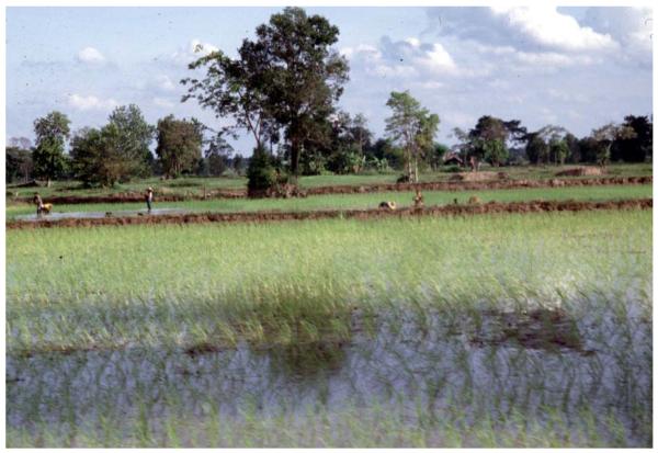
Land cover classifications of satellite imagery in Nang Rong, especially historical images, are complicated by several factors. First, Landsat Multispectral Scanner (MSS) data became available in 1972 and Landsat Thematic Mapper (TM) data began being collected in 1982. The sensor systems of each have different spatial, spectral, temporal, and radiometric resolutions to characterize the Earth, introducing noncomparabilities into the image time series.⁵ Second, cloud-free images are available primarily during the dry season, as clouds and the shadows that they cast obscure information about the landscape, when data from optical remote sensing systems are used. The spectral response differences are considerable between the wet and dry periods in northeastern Thailand. However, the cloud-free period in northeastern Thailand corresponds to the monsoonal dry period of approximately December through April, when the lowland paddy rice has been harvested and only crop stubble remains and when differences between a harvested rice field and another harvested crop type are more difficult to discern. Third, trees dot the rice fields throughout the district. Figure 6 illustrates this with a recent ground photograph. Because of the size of the trees relative to the pixel dimensions of Landsat MSS and TM, an integrated pixel response pattern results in which the landscape features that comprise the landscape combine to derive a composite pixel of a collection of landscape features, such as trees, rice paddies, and water, and not a singular type of land cover. Fourth, although seasonality in rice cultivation is pronounced and somewhat predictable, the same cannot be said of the other crops grown in Nang Rong. Cassava, in particular, can be planted throughout the year, and it can be harvested any time between 9 and 15 months later. Also, depending upon local site conditions set by topography, soil moisture, soil type and so on, spectral separation of the same crop type and different crop types is not a straight-forward activity, particularly, when detailed land cover information is the goal of the satellite image processing. Finally, the Northeastern region is marked by variability in timing and amount of precipitation, thereby changing the crop phenology and the spectral response patterns across the landscape, and particularly across an image time-series.

Fig. 6.

Rice paddy in Nang Rong.

With these reservations in mind, the top panel of Table 1 compares the percent in forest simulated for each of the four scenarios to the percent in forest according to the satellite classifications. If we conduct an endpoint comparison, we would identify Scenario B as coming the closest to the percent of forest in the satellite classification for 1999. However, simulations of trends in forest cover based on Scenario B do not consistently outperform the others. Scenario C comes closest in four of comparisons (1972, 1975, 1985, and 1995), Scenario B in two of the comparisons (1988 and 1999), and Scenario D in one (1996). If we examine all of the comparisons in the table, we would identify Scenario C as most closely reproducing the trend in forest cover shown in the satellite images, although as noted above, differences between scenarios are not large.

Differences across scenarios are more pronounced for rice and upland crops than for forest. For rice, as shown in the second panel of Table 1, simulations based on Scenario C outperform those based on any other scenario for all years shown except for the last, when Scenario A does a bit better. For cassava and other upland crops, as shown in the bottom panel, it varies. Scenario B comes the closest early in the period (1972, 1975), Scenario A in the middle (1985, 1988, 1995), and Scenario C at the end (1996, 1999). It is thus important to consider all of the years, not just the endpoint. Considering all three classes–forest, rice, and upland crops–Scenario C does the best job reproducing estimates based on satellite imagery. Scenario C incorporates a contemporaneous primary effect of village settlement, i.e., one that begins with the formal establishment of the village, and a lagged secondary effect.

Sensitivity testing

We use the CA model as a kind of laboratory in which to study the implications of our hypotheses about village settlement over this period. Scenarios A-D were designed to examine differences in the timing of the primary settlement effect and the existence of a secondary settlement effect. In all of the scenarios, however, the maximum spatial extent of these effects is fixed: 1.5 kilometers for the primary effect and 0.25 kilometers for the secondary effect. In this section, we examine the sensitivity of results to these assumptions. Because we did not start with a specific interest in the areal extent of primary and secondary settlement effects, we view this as sensitivity testing rather than hypothesis testing.

We examine five alternative assumptions about the areal extent of village settlement effects. The assumption about the spatial extent of the primary settlement effect in Scenarios A-D is based on the distance a farmer could easily travel under a hot equatorial sun, carrying his or her agricultural implements. We estimated this distance to be 1.5 kilometers, but a shorter distance of 1.0 kilometers might be argued in the absence of roads, common in the earlier part of the period under consideration. Alternatively, if a road system is in place and vehicular transport common, a circumstance that prevailed in the latter part of the period, a longer distance of 2.0 kilometers might be argued. The assumption about the spatial extent of the secondary settlement effect is based on the highly clustered and relatively small number of dwelling units found in a typical village. We estimated this distance to be 0.25 kilometers, but for larger and more dispersed villages, it might be 0.50 kilometers. Relaxing assumptions about the areal extent of primary and secondary settlement effects in the original CA model yields three values for the extent of the primary effect–1.0, 1.5, and 2.0 kilometers–and two values for the extent of the secondary effect–0.25 and 0.50 kilometers. In the sensitivity testing, we consider all possible pairs except for a primary effect of 1.0 kilometers paired with a secondary effect of 0.50 kilometers, a set of values that is nonsensical. All sensitivity testing is based on Scenario C.

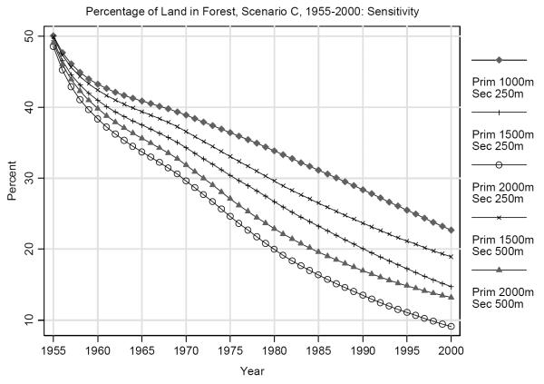
Figure 7 shows the trends in forest cover associated with five different assumptions about the extent of the primary and secondary effects of village settlement. The differences associated with assumptions about the spatial extent of the village settlement shown in Figure 7 are larger than the differences associated with the timing of the primary effect and the existence of the secondary effect shown in Figure 3. Assuming a more limited primary settlement effect of 1.0 rather than 1.5 kilometers, and keeping the secondary settlement effect at 0.25 kilometers, leads to a simulated landscape that is 23 rather than 15 percent in forest cover in 2000. Assuming a more expansive primary settlement effect of 2.0 kilometers rather than 1.5 kilometers, and keeping the secondary settlement effect at 0.25 kilometers, leads to a simulated landscape that is 9 rather than 15 percent in forest in 2000. These are substantial differences. The trend lines show that with respect to landscape composition, the results are most sensitive to the extent of the primary settlement effect. The assumptions embedded in the earlier scenario testing are associated with the trend line in the middle. The trend line marked with black diamonds at the top of the graph assumes a more limited primary effect. The trend line marked with circles at the bottom of the graph assumes a broader primary effect. The trend lines associated with different assumptions about the secondary effect are in the middle.

Fig. 7.

Percentage of land in forest, scenario C, 1955-2000: Sensitivity.

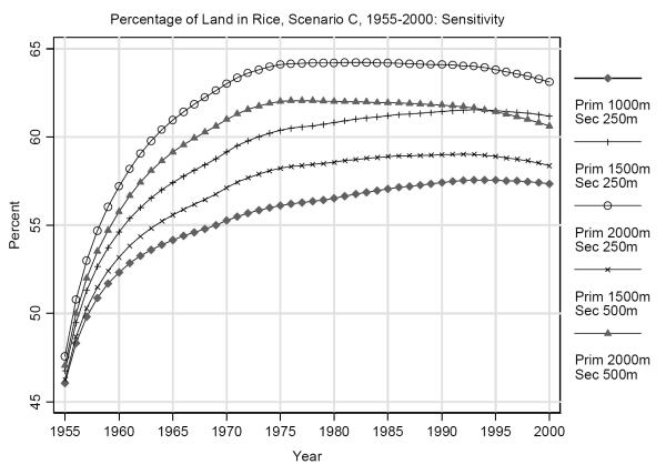
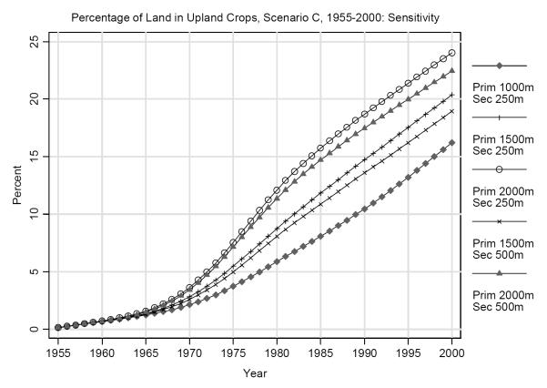
Figures 8 and 9 show a similar picture for rice and upland crops, although importantly, variation associated with the sensitivity testing is less than that associated with the scenarios examined earlier. Earlier, there was a ten percentage point difference separating the simulated fractions in rice (Figure 4). Here, there is a six point difference. Earlier, there was a ten percentage point difference separating the simulated fractions in cassava and other upland crops (Figure 5). Here there is an eight point difference.

Fig. 8.

Percentage of land in rice, scenario C, 1955-2000: Sensitivity.

Fig. 9.

Percentage of land in forest, Scenario C, 1955-2000: Sensitivity.

Overall, the simulations are sensitive to the spatial extent of the primary and secondary settlement effects as well as to their timing. This makes sense, given the increasing numbers and dispersal of villages over the period studied. Do any of the alternative assumptions about the spatial extent of the settlement effects do a better job than our original assumptions? An initial response to this question compares the simulated landscape composition in 1999 based on different assumptions about spatial extent to the satellite land cover classification for that year. With respect to the percent of land in forest cover, allowing for a larger spatial extent (2.0 km, 0.50 km.) comes a little closer to the satellite land cover classification than our original assumptions (1.5 km., 0.25 km.), but not by much. Our original assumptions are best for rice. A larger secondary effect (1.5 km., 0.50 km.) comes closest for cassava and upland crops. We conclude that our original assumptions are reasonable.

Although initially conceptualized as a sensitivity test, the results point to some potentially interesting conclusions worth following up more formally. If Nang Rong had remained isolated throughout the second half of the 20^th century, with little road development, and reliance on hand tools for agriculture, the spatial extent of village settlement effects would have been more limited. Deforestation would have been less, with correspondingly less land in rice and upland crops by 2000. If Nang Rong had been already integrated in the national and international economy in 1954, with a well established road system, and tractors, trucks, and itans, the spatial extent of village settlement would have been greater. Deforestation would have occurred more quickly, with proportionally more land in rice and upland crops. Neither was the case. Rather, as described earlier, road construction, the mechanization of agriculture, and the integration of Nang Rong into the larger economy happened over the period. We will construct scenarios to capture these changes in future work with our CA models, but the results here indicate how population growth (in the form of village settlement) and technology relate to one another in non-linear ways to influence land cover change.

IMPLICATIONS

Frontiers provide opportunities to test core hypotheses about human population dynamics and changes in land cover (Gutmann et al., 2005). In the context of frontier settlement and agricultural transformation, it is possible to see how people manipulate the land and their lives given social, cultural, economic, and environmental constraints. This paper examined frontier settlement and land cover change over the last half century in Nang Rong, a district in Northeast Thailand. Within the context of a Cellular Automata (CA) model, we explored the implications of village settlement for deforestation and the extensification of agriculture in a frontier setting.

Our main focus was village settlement effects. In Nang Rong, villages are clusters of dwelling units surrounded by agricultural lands. First, we hypothesized that forest located in and around the center of settlement would be converted to agricultural use in inverse relationship to distance from the center, depending on biophysical conditions. We called this a primary effect. Second, we hypothesized that once a village is established, after a lag, forest cover would reappear within the center of the village. We called this a secondary effect. Four scenarios were designed to assess different pairs of primary and secondary effects. The results of simulations suggest the importance of the primary effect, especially its timing, for landscape composition in the history of Nang Rong, Thailand over the past half century.

Our hypotheses about the impact of village settlement assume a particular spatial organization to settlement patterns. Whether primary or secondary, the impact of settlement on land cover is presumed to radiate outwards from the village center. In other settings, even in other parts of Thailand, settlement is more dispersed. In the areas of the Amazon where governmentally planned settlement occurred, for example, areas for settlement were laid out in a grid, with households residing on as well as farming their plots (Thapa and Bilsborrow, 1994; Moran et al., 1994). The impact of settlement on land cover is likely to look quite different in such settings, e.g., following roads, gradually seeping outwards (e.g., Messina and Walsh, 2001). The impact of settlement in frontier settings thus depends on the sociospatial organization of settlement itself, which varies by setting.

Even though this is a CA model rather than an agent-based model, the rules built into the CA model are based on how we think agents behave, and so here we use the language of agents and their behavior. From this perspective, hypotheses about the timing of primary and secondary village settlement effects are about the relationship between land cover change and the temporal behavior of agents. We tested the sensitivity of the results to assumptions about the spatial extent of village settlement effects. We took Scenario C, which is the one that best matched the series of satellite classifications, and varied the spatial extent of the agent’s influence on the landscape, both the extent to which they moved from the village center to farm and the extent of the shade and fruit tree cover around the nucleated set of dwelling units. Model variation in land cover change is more sensitive to the spatial reach of village households than their temporal reach. While our initial assumptions about the spatial extent of the settlement effect turned out to be quite reasonable, the sensitivity of the model to these assumptions points to an important area for further research. The fact that the spatial reach of village households is directly tied to the size, quality, and connectivity of the road system as well as access to vehicles such as mopeds and trucks makes this all the more interesting aspect of the model to explore.

In looking at settlement processes in relation to land cover change, we have taken the location of human settlement as given, changing over the period but exogenous with respect to land cover change. This is typical of the broader literature as well. However, in many cases, including the recent history of Nang Rong, settlement is “spontaneous,” with the timing and spatial pattern of settlement determined by choices made by settlers as they occupy the land and convert it to agricultural use. Sites are chosen, or not, depending on their characteristics. Households form, new households move in, and populations grow as a result of the opportunities represented in the landscape and its change. Conversely, opportunities anticipated but not present in the new areas can lead individuals and households to leave. Although often treated in the literature as an exogenous driver of land cover change, population is clearly endogenous to land cover change. A major next step in the development of our model is to incorporate village location as an outcome of land cover as well as determinant of it. Where people choose to settle as well as whether those places grow, are stable, or decline, depends on resource endowments, land availability, connections to other places, local infrastructure, social ties and technological changes. The impact of those choices on land cover depends on these same characteristics.

Even though we were able to build into our CA model our expectations as to how people behave under changing circumstances, our work with CA models (also see Walsh et al., 2006) has convinced us that CA models work best when examining the long term impacts of exogenous factors, but not so well when examining the changing behavior of agents within a study area, especially in the short term. For the latter, we think the next logical step is to incorporate some spatially explicit agent-based modeling components, bringing in the dynamic interrelationships among migration, household assets, and land use within the larger and changing social and biophysical environment. In work just beginning, we are using agent-based models to link changes in household membership, use of specific land parcels, and household wealth to be able to better understand the feedbacks among these processes as they relate to land use change.

APPENDIX. CA Model Description

The model simulates yearly growth and change from 1954 to 2000 among three land cover classes in Nang Rong district: rice, upland crops, and forest. The model operates on 1,485,427 30 × 30 m cells, with a land cover state assigned to each cell. The core of the model consists of an iterative process in which each of the three modeled classes “grows” new cells, then cells assigned to more than one class are reconciled based on land cover suitabilities to determine each cell’s output land cover state for that year, which is then used as the input for the subsequent year. This process is described in more detail in what follows.

Model initialization

The model initializes by importing the 1954 forest/rice land cover data layer derived from aerial photography. It also imports GIS data layers used as components for calculating a land use suitability score for the three modeled classes for each cell. Static score components do not change from year to year, such as landform characteristics or slope angle. Dynamic components change over time as the landscape changes, such as distance to the nearest village as new villages appear in the district.

Start iteration

Separate into classes and grow. At the start of each iteration, individual class layers are extracted from the model output from the previous year (or from the starting land cover classification for the first iteration).

For each class, a small number of cells are randomly seeded as new cells of the class being operated on. These are added to the output from the previous iteration. The proportion of cells randomly selected to be included is an adjustable parameter, and may be spatially stratified within the simulated landscape. This is used as the input to the morphological dilation operator, which “grows” new cells of the class. In the dilation process, a small kernel (3×3 cells) is passed over the input data. An adjustable threshold value determines whether the focal cell in the kernel will change based on whether enough (i.e. greater than or equal to the threshold number) cells within the kernel are already of that class type. This threshold value may vary based on location, e.g. at different distances from village centroids.

Calculate suitability scores

For each cell, a companion score is calculated for each of the three modeled classes. These scores are based on the static and dynamic inputs indicating the land use suitability of the cell for that class: rice, upland crops, or forest.

Rice suitability scores are calculated based on slope angle, landform morphology, distance to water, soil moisture and quality characteristics, and distance to the nearest village. Upland crop suitability scores are based on slope angle, landform morphology, soil moisture and quality characteristics, and distance to the nearest village. Forest suitability scores are calculated based on slope angle, landform morphology, distance to water, and distance to the nearest village.

Finish iteration

Reconcile new growth.

After new growth for each class is modeled separately, some cells will be flagged as potential members of only one class (either still “on” or newly “turned on” in that class), while others will be flagged for multiple classes. For those cells that are in competition between multiple classes, the model compares the scaled (0 to 1) suitability scores for each class in order to select among them. In most cases, the highest score “wins.”

However the suitability scores are clearly estimates, and the land use decision makers operate with incomplete and inexact information and so may make suboptimal decisions. So we define an adjustable uncertainty interval in which the scaled scores for each class are considered too close to make a call. Within that interval, the output land cover state is randomly chosen from the classes in competition.

After new growth reconciliation, the land cover state for each cell is saved, and then passed to the next iteration until the final year of the simulation is reached.

REFERENCES

- Bak P. How Nature Works. Copernicus/Springer-Verlag; New York: 1998. [Google Scholar]
- Batty M, Xie Y, Sun Z. Modeling urban dynamics through GIS-based cellular automata. Computers, Environment and Urban Systems. 1999;23:205–233. [Google Scholar]
- Bian L. Multiscale nature of spatial data in scaling up environmental models. In: Quattrochi DA, Goodchild MF, editors. Scale in Remote Sensing and GIS. Lewis Publishers; New York: 1997. pp. 13–26. [Google Scholar]
- Brondizio ES, McCracken SD, Moran EF, Siqueira AD, Nelson DR, Rodriguez-Pedraza C. The colonist footprint: toward a conceptual framework of deforestation trajectories among small farmers in frontier Amazonia. In: Wood C, Porro R, editors. Deforestation and Land Use in the Amazon. University Press of Florida; Gainesville: 2002. pp. 133–161. [Google Scholar]
- Brown DG, Page S, Riolo R, Zellner M, Rand W. Path dependence and the validation of agent-based spatial models of land use. International Journal of Geographical Information Science. 2005;19(2):153–174. [Google Scholar]
- Cilliers P. Complexity and Postmodernism. Routledge; New York: 1998. [Google Scholar]
- Coale AJ. The Growth and Structure of Human Population; A Mathematical Investigation. Princeton University Press; Princeton, N.J.: 1972. [Google Scholar]
- Crawford TW, Messina JP, Manson SM, O’Sullivan D. Complexity science, complexity systems and land use research. Environment and Planning B. In press. [Google Scholar]
- Deadman P, Robinson D, Moran E, Brondizio E. Colonist household decision-making and land-use change in the Amazon Rainforest: an agent-based simulation. Environment and Planning B. 2004;31:693–709. [Google Scholar]
- Entwisle B, Edmeades J, Malanson G, Podhisita C, Prasartkul P, Rindfuss RR, Walsh SJ. Village Settlement, Deforestation, and the Expansion of Agriculture in a Frontier Region: Nang Rong, Thailand. In: Jepson W, Millington A, editors. Changing Countrysides: Dynamics of Land Modification in the Tropics. Springer; Forthcoming. Forthcoming. [Google Scholar]
- Entwisle B, Stern PC, editors. Population, Land Use, and Environment: Research Directions. National Academy Press; Washington, DC: 2005. [PubMed] [Google Scholar]
- Entwisle B, Walsh SJ, Rindfuss RR, VanWey LK. Population and upland crop production in Nang Rong, Thailand. Population and Environment. 2005;26(6):449–470. [Google Scholar]
- Foster AD, Rosenzweig MR, Behrman JR. Population, income, and forest growth: management of village common land in India. 2003. Unpublished manuscript.
- Fukui J. Food and population in a Northeast Thai village. University of Hawaii Press; Honolulu: 1993. [Google Scholar]
- Gell-Mann M. The Quark and the Jaguar. Freeman; New York: 1994. [Google Scholar]
- Gutmann MP, Pullum-Pinon SM, Witkowski K, Deane GD. Land use and the family cycle in the settlement of the U.S. Great Plains. 2005. Unpublished manuscript. [DOI] [PMC free article] [PubMed]
- Holland JH. Emergence: From Chaos to Order. Helix; Reading, MA: 1998. [Google Scholar]
- Ingram J. Economic Change in Thailand 1850-1970. Stanford University Press; Stanford: 1971. [Google Scholar]
- Kanae S, Oki T, Musaike K. Impact of deforestation on Regional Precipitation over the Indochina Peninsula. Journal of Hydrometeorology. 2001;2:51–70. [Google Scholar]
- Liu J, Ouyang Z, Tan Y, Yang J, Zhou S. Changes in human population structure and implications for biodiversity conservation. Population and Environment. 1999;21:45–58. [Google Scholar]
- Liu J, Daily G, Ehrlich P, Luck G. Effects of household dynamics on resource consumption and biodiversity. Nature. 2003;421:530–533. doi: 10.1038/nature01359. [DOI] [PubMed] [Google Scholar]
- Luhman N. A Sociological Theory of Law. Routledge and KeganPaul; London: 1985. [Google Scholar]
- Malanson GP. Considering complexity. Annals, Association of American Geographers. 1999;89:746–753. [Google Scholar]
- Malanson GP, Zeng Y, Walsh SJ. Complexity at advancing ecotones and frontiers. Environment and Planning A. 2006;38:619–632. [Google Scholar]
- Manson SM. Simplifying complexity: a review of complexity theory. Geoforum. 2001;32(3):405–414. [Google Scholar]
- Manson SM. Validation and verification of multi-agent models for ecosystem management. In: Janssen M, editor. Complexity and Ecosystem Management: The Theory and Practice of Multi-Agent Approaches. Edward Elgar Publishers; Northampton, Massachusetts: 2003. pp. 63–74. [Google Scholar]
- Mas JF, Puig H, Palacio JL, Sosa-Lopez A. Modeling deforestation using GIS and artificial neural networks. Environmental Modeling & Software. 2004;19:461–471. [Google Scholar]
- Matthews KB, Subaald AR, Craw S. Implementation of a spatial decision support system for rural land use planning: integrating geographic information systems and environmental models with search and optimization algorithms. Computers and Electronics in Agriculture. 1999;23:9–26. [Google Scholar]
- McCracken SD, Brondizio ES, Nelson DR, Moran EF, Siqueira AD, Rodriguez-Pedraza C. Remote sensing and GIS at the farm property level: demography and deforestation in the Brazilian Amazon. Photogrammetric Engineering and Remote Sensing. 1999;65:1311–1320. [Google Scholar]
- Messina JP, Walsh SJ. 2.5D morphogenesis: modeling landuse and landcover dynamics in the Ecuadorian Amazon. Plant Ecology. 2001;156:75–88. [Google Scholar]
- Messina JP, Walsh SJ. Dynamic spatial simulation modeling of the population-environment matrix in the Ecuadorian Amazon. Environment and Planning B. 2005;32(6):835–856. [Google Scholar]
- Parker DS, Manson SM, Janssen M, Hoffmann M,P, Deadman P. Multi-agent systems for the simulation of land use and land cover change: a review. Annals of the Association of American Geographers. 2003;93(2):314–337. [Google Scholar]
- Moran EF, Brondizio E, Mausel P, Wu Y. Integrating Amazonian vegetation, landuse, and satellite data. Bioscience. 1994;44:329–338. [Google Scholar]
- National Research Council (NRC) Grand Challenges in Environmental Sciences. National Academy Press; Washington, DC: 2001. [Google Scholar]
- Phongphit S, Hewison K. Village Life: Culture and Transition in Thailand’s Northeast. White Lotus; Bangkok: 2001. [Google Scholar]
- Riethmuller R, Scholz U, Sirisambhand N, Spaeth A. Spontaneous land clearing in Thailand: the Khorat Escarpment and the Chonburi Hinterland. In: Uhlig H, editor. Spontaneous and Planned Settlement in Southeast Asia. Institute of Asian Affairs; Hamburg: 1984. pp. 119–248. [Google Scholar]
- Rindfuss RR, Walsh SJ, Turner BL, II, Fox J, Mishra V. Developing a Science of Land Change: Challenges and Methodological Issues. Proceedings of the National Academy of Science. 2004;101(939):13976–13981. doi: 10.1073/pnas.0401545101. [DOI] [PMC free article] [PubMed] [Google Scholar]
- Siamwalla A. Four Episodes of Economic Reform in Thailand 1958-1992. Thailand Development Research Institute; Bangkok: 1995. [Google Scholar]
- Silveira B, Coutinho G, Lopes C. DINAMICA - a stochastic cellular automata model designed to simulate the landscape dynamics in an Amazonian colonization frontier. Ecological Modelling. 2002;154(3):217–235. [Google Scholar]
- Snyder F. European Community Law and International Economic Relations: The Saga of Thai Manioc. European University Institute; San Domenico: 1993. [Google Scholar]
- Thapa KK, Bilsborrow RE. Frontier migration and environmental degradation in developing countries: experiences from Nepal and Ecuador. In: Clarke JI, Tabah L, editors. Population-Environment-Development Interactions. CICRED; Paris: 1994. pp. 253–271. [Google Scholar]
- VanLandingham M, Hirschman C. Population pressure and fertility in pre-transition Thailand. Population Studies. 2001;55:233–248. doi: 10.1080/00324720127694. [DOI] [PubMed] [Google Scholar]
- Walsh SJ, Entwisle B, Rindfuss RR, Page PH. Spatial simulation modeling of land use/land cover change scenarios in Northeastern Thailand: a cellular automata approach. Journal of Land Science. 2006;1(1):5–28. [Google Scholar]
- Webster CJ, Wu F. Regulation, land use mix and urban performance. Part 2: simulation. Environment and Planning A. 1999;31:1529–1545. [Google Scholar]
- White R, Engelen G. Cellular automata and fractal urban form: a cellular modeling approach to the evolution of urban landuse patterns. Environment and Planning A. 1993;25:1175–1199. [Google Scholar]
- White R, Engelen G, Uljee I. The use of constrained cellular automata for high-resolution modeling of urban land-use dynamics. Environment and Planning B. 1997;24:323–343. [Google Scholar]