Neural and Hemodynamic Responses Elicited by Forelimb- and Photo-stimulation in Channelrhodopsin-2 Mice: Insights into the Hemodynamic Point Spread Function

Abstract

Hemodynamic responses are commonly used to map brain activity; however, their spatial limits have remained unclear because of the lack of a well-defined and malleable spatial stimulus. To examine the properties of neural activity and hemodynamic responses, multiunit activity, local field potential, cerebral blood volume (CBV)-sensitive optical imaging, and laser Doppler flowmetry were measured from the somatosensory cortex of transgenic mice expressing Channelrhodopsin-2 in cortex Layer 5 pyramidal neurons. The magnitude and extent of neural and hemodynamic responses were modulated using different photo-stimulation parameters and compared with those induced by somatosensory stimulation. Photo-stimulation-evoked spiking activity across cortical layers was similar to forelimb stimulation, although their activity originated in different layers. Hemodynamic responses induced by forelimb- and photo-stimulation were similar in magnitude and shape, although the former were slightly larger in amplitude and wider in extent. Altogether, the neurovascular relationship differed between these 2 stimulation pathways, but photo-stimulation-evoked changes in neural and hemodynamic activities were linearly correlated. Hemodynamic point spread functions were estimated from the photo-stimulation data and its full-width at half-maximum ranged between 103 and 175 µm. Therefore, submillimeter functional structures separated by a few hundred micrometers may be resolved using hemodynamic methods, such as optical imaging and functional magnetic resonance imaging.

Introduction

Noninvasive methods to investigate brain function in humans, such as functional magnetic resonance imaging (fMRI), rely on activation-evoked regional changes in blood oxygenation. It is well known that these changes in blood oxygenation result from those in cerebral blood flow (CBF), blood volume, and oxygen consumption (Ogawa et al. 1993; Buxton et al. 1998; Davis et al. 1998; Kim et al. 1999; Kim and Ogawa 2012). Understanding the relationship between these hemodynamic changes and their neural activity has been crucial for the proper interpretation of brain imaging data. Significant progress has been attained in understanding the temporal properties of this neurovascular relationship; for example, linear and nonlinear characteristics have been observed between evoked activity and the hemodynamic response (Boynton et al. 1996; Vazquez and Noll 1998; Logothetis et al. 2001; Martindale et al. 2005; Sanganahalli et al. 2009; Rios et al. 2010). Concurrent imaging and electrophysiological experiments have shown that the magnitude of temporal hemodynamic changes at the recording site is well correlated with field potential activity and spiking activity (Ogawa et al. 2000; Logothetis et al. 2001). Spatially, hemodynamic responses are known to over-extend the neurally active tissue (Malonek and Grinvald 1996; Berwick et al. 2008; Vazquez et al. 2010). However, the spatial specificity of hemodynamic changes has also been demonstrated in relatively small scales using small functional structures, such as individual whisker barrels in rats and orientation domains in the cat visual cortex (Yang et al. 1996; Duong et al. 2001; Weber et al. 2004; Zhao et al. 2005; Moon et al. 2007; Berwick et al. 2008). Nevertheless, the spatial properties of the neurovascular coupling have remained unclear, particularly over submillimeter scales, because of the lack of a well-defined and malleable spatial stimulus. Uncovering and understanding the spatial properties of the neurovascular coupling are essential to fully exploit hemodynamic signals and in their use for interpreting brain function (i.e. neural activity), particularly with the increasing use of new image acquisition methods with submillimeter resolution.

Mice expressing Channelrhodopsin-2 (ChR2) have been developed as part of the optogenetics toolset with the expression of ChR2 throughout the cortex (Wang et al. 2007), presenting a potentially ideal model to spatially and temporally modulate neuronal activity. This animal model possesses several important properties. First, increases in the light- or photo-stimulation intensity have been shown to increase the current of patched cells by the increased recruitment of photoreceptors (Wang et al. 2007). Interestingly, ChR2 can depolarize ChR2-positive neurons to fire action potentials with bright light flashes, while dim light flashes cause subthreshold depolarizations. More importantly, the number of evoked action potentials is proportional to the photo-stimulus intensity. Secondly, the expression of ChR2 is mediated by the Thy1 promoter and its presence in the cortex is limited to Layer 5 pyramidal neurons and their processes that extend to superficial layers (Wang et al. 2007). Nevertheless, this animal model has been used by several groups to show that photo-stimulation is capable of eliciting spatially selective neuronal activity as well as detectable hemodynamic responses (Ayling et al. 2009; Kahn et al. 2011; Scott and Murphy 2012). In these studies, hemodynamic responses induced by photo-stimulation were reported to extend over 1 mm (Desai et al. 2011; Scott and Murphy 2012). Thirdly, the presence of ChR2-positive cells in these mice is conveniently identified by the coexpression of yellow fluorescent protein (YFP) (Wang et al. 2007). Therefore, this optogenetic model can be used to identify and to spatially manipulate neural activity in a spatially selective neuronal population by modulating the photo-stimulation parameters.

ChR2 transgenic mice were used in this work to investigate the relationship between neural activity and hemodynamic responses evoked by forelimb- and photo-stimulation, particularly in the spatial dimension. A metal electrode was used to measure the evoked local field potential (LFP) and multiunit activity (MUA), while optical imaging of intrinsic signal (OIS) and laser Doppler flowmetry (LDF) were used to measure hemodynamic responses. Both the intensity and duration of photo-stimuli were used to modulate the extent and spiking rate of the targeted area, centered at the forelimb area in the somatosensory cortex. Potential differences in the activity evoked by the forelimb versus photo-stimulation may limit the ability of this optogenetic model to elucidate on the relationship between neural activity and hemodynamic responses. Therefore, the following measurements were performed to compare these 2 pathways and their neurovascular relationships: (1) Depth profile of neural activity induced by forelimb- and photo-stimulation, (2) magnitude of the neural activity and hemodynamic responses, and (3) spatial extent of hemodynamic responses relative to spatial estimates of neural activity. The data collected were then used to determine the magnitude and spatial properties of hemodynamic responses as a function of neural activity as well as to estimate its point spread function (PSF).

Materials and Methods

A total of 19 adult mice obtained from the Jackson Laboratory (Bar Harbor, ME, USA) were used. Fifteen transgenic mice (23–32 g; 2–7 month old) expressing ChR2 throughout their central nervous system [n = 10 for strain B6.Cg-Tg(Thy1-COP4/EYFP)9Gfng/J and n = 5 for strain B6.Cg-Tg(Thy1-COP4/EYFP)18Gfng/J] were used for the experimental group, and 4 adult mice (24–35 g, 2–8 month old; n = 2 for C57BL6/J and n = 2 for B6.Cg-Tg(Thy1-eGFP)OJrs/GfngJ) were used as a control group. All procedures performed followed an experimental protocol approved by the University of Pittsburgh Institutional Animal Care and Use Committee in accordance with the standards for humane animal care and use as set by the Animal Welfare Act and the National Institutes of Health Guide for the Care and Use of Laboratory Animals. The animals were initially anesthetized using a ketamine (75 mg/kg) and xylazine (10 mg/kg) or dex-dormitor (0.5 mg/kg) cocktail administered intraperitoneally (IP). An IP line was then inserted to administer fluids (5% dextrose in saline) as well as supplementary anesthesia throughout the experiment, which consisted of ketamine alone at 30 mg/kg/h, typically commencing about 1 h after induction. Two needle electrodes were placed in the left forepaw between digits 2 and 4 for electrical stimulation (Silva et al. 1999). The animals were then placed in a stereotaxic frame (Narishige, Tokyo, Japan), and supplementary oxygen was administered “blow-by” using a cannula at a rate of 500 mL/min. The heart rate was continuously monitored throughout the experiment using metal leads placed subcutaneously in the abdomen to assess the physiological condition of the animal and depth of anesthesia. Body temperature was maintained at 37°C using a thermal probe and heating pad controlled by a direct current feedback unit (40-90- 8C; FHC, Inc., Bowdoinham, ME, USA). The thermal probe was placed under the abdomen, and a small blanket was placed over the animal to help maintain the animal's temperature throughout the experiment. Heart rate and body temperature were recorded using a polygraph data acquisition software (Acknowledge, Biopac Systems, Inc., Goleta, CA, USA). The skull was then exposed over the somatosensory area. A well was made using acrylic cement surrounding an area about 4 × 3 mm² on the right side of the skull, centered about 2 mm lateral and 1 mm rostral from the bregma. The skull in this area was then removed using a dental drill, and cerebrospinal fluid was released around the cisterna magna area to minimize herniation. Surgical light exposure to the brain during and after the craniotomy was filtered to green-yellow light (570 ± 10 nm) to avoid exposure to white light, which could continuously stimulate the exposed brain tissue. The well area was then filled with 1% agarose gel at body temperature.

Probe Placement

The location of the forelimb area was then identified for electrode and probe placement using OIS at a wavelength of 572 nm (Fig. 1A). This wavelength corresponds to an isosbestic point for hemoglobin, making the OIS data sensitive to changes in total amount of hemoglobin and therefore representative of cerebral blood volume (CBV). OIS data were acquired at 30 frames per second (fps) using an analog CCD camera (Sony XT-75, Japan) and an A/D frame-grabbing board (Matrox, Inc., Dorval, Quebec, Canada) over a field-of-view of 3.5 × 3.0–4.4 × 3.7 mm² depending on the magnification setting of the macroscope (MVX-10; Olympus, Tokyo, Japan). The light source consisted of oblique light guides connected to a halogen light source (Thermo-Oriel, Stratford, CT, USA) to transmit filtered light at a wavelength of 600 ± 50 nm. A barrier filter (572 ± 7 nm) was placed prior to the camera to obtain the desired CBV sensitivity. The forelimb stimulus consisted of 1.5 mA, 0.5-ms electrical pulses at a frequency of 5 Hz for 4 s every 16 s, repeated 10 times. The stimulus was delivered using a current isolator box (AMPI, Jerusalem, Israel) driven by a Master-8 waveform generator (AMPI, Jerusalem, Israel). Forelimb area maps were generated by computing an average difference image of the data obtained over each stimulation trial and the data from each 2-s period preceding stimulation onset (−3 to −1 s).

Figure 1.

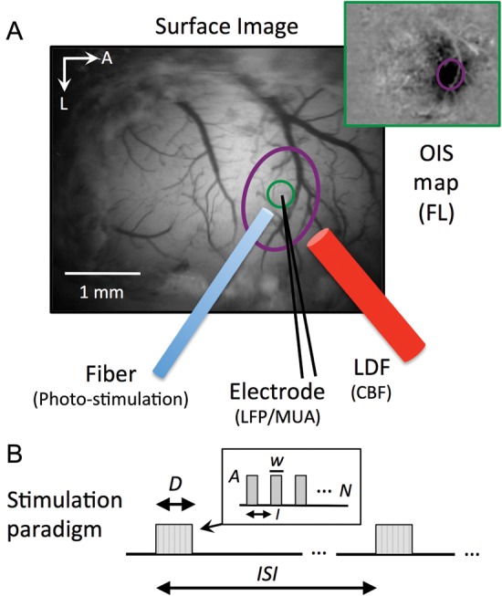
Experimental set-up and stimulation paradigm. (A) Experimental set-up for electrophysiological recording, hemodynamic data acquisition, and photo-stimulation. Following the craniotomy, an OIS experiment was performed to map the forelimb somatosensory area (top-right inset, purple ovals) and place a metal electrode, optic fiber, and LDF probe. The metal electrode was used to record LFP and MUA, the optic fiber was used for photo-stimulation, OIS was used to image hemodynamic CBV responses, and LDF was used to measure hemodynamic changes in CBF. A circular ROI (green circle) was used to extract time series from the CBV-sensitive OIS data. (B) Diagram of the experimental paradigm used for stimulation. For Experiment 1, single electrical or photo-stimulation pulses were delivered every 3 s (number of pulses N = 1, ISI = 3 s). For Experiment 2, electrical or photo-stimulation pulses were delivered for 4 s at a frequency of 5 Hz every 60 s (number of pulses N = 20, interval I = 200 ms, stimulus duration D = 4 s). The amplitude (A) and duration (w) of each pulse were varied depending on the stimulus. OIS: optical imaging of intrinsic signal; LDF: laser Doppler flowmetry; CBV: cerebral blood volume; CBF: cerebral blood flow; ROI: region of interest; LFP: local field potential; MUA: multiunit activity; N: number of pulses; I: interval; ISI: interstimulus interval; D: stimulus duration; A: pulse amplitude; w: pulse width.

An optic fiber, metal electrode, and LDF probe were placed as close as possible to the hotspot location while avoiding large surface vessels. The optic fiber used to deliver the photo-stimulus has a core diameter of 125 µm (S-405-HP, ThorLabs, Inc., Newton, NJ, USA). The metal electrode (Carbostar-1 with a tip diameter of 5 µm and resistance of about 1 MΩ; Kation Scientific, Minneapolis, MN, USA) was placed adjacent to the optic fiber below the core of the illuminated area at a depth of 260 µm. Lastly, the LDF (Perimed, Inc., Jarfalla, Sweden) probe used has a tip diameter of 450 µm and operating wavelength of 780 nm. It was placed over the area illuminated by the optic fiber and the location of the metal electrode to monitor and record CBF. Because each probe was placed under the optical imaging system, the fiber, electrode, and probe were inserted at a 60° angle. This set-up was allowed to settle for 15 min, after which the experimental data acquisition commenced. The location of the optic fiber and LDF probe was fixed throughout the experiments.

Experimental Design

Photo-stimulation and forelimb stimulation experiments were performed as follows. The photo-stimulus was delivered using a power-adjustable, transistor-transistor logic (TTL)-controlled, 473 nm laser diode unit (CrystaLaser, Inc., Reno, NV, USA) connected to the optic fiber. Since the brain is a relatively high light-scattering medium, increasing the intensity of photo-stimulation increases the spatial extent of the stimulus and also the spike rate. Increasing the photo-stimulus duration is expected to increase the spike rate and have a smaller impact on spatial extent. Therefore, 6 photo-stimulation parameters sets were used: 1.0, 0.5, and 0.25 mW pulses [measured at the end of the fiber using a power meter (Melles Griot 13PEM001, CVI Melles Griot, Inc., Alburquerque, NM, USA)] with duration of 10 ms, 1.0 and 0.25 mW pulses with duration of 30 ms, and 1.0 mW pulses with duration of 2 ms. In comparison, responses obtained by forelimb stimulation using 1.5 mA, 0.5 ms electric pulses were also recorded. Electrophysiological activity was recorded at a frequency of 20 kHz (MAP, Plexon, Inc., Dallas, TX, USA). OIS was recorded at 30 fps and LDF at 1 kHz.

Two experimental sessions were performed in most of the animals as described below. The total number of animals used for each experimental session is indicated in Table 1.

Table 1.

Number of subjects for each experiment

Photo-stimulation		Experiment 1		Experiment 2
Amplitude	Duration	LFP & MUA center	LFP & MUA distance (a)	OIS and LFP & MUA	OIS only
1.0 mW	30 ms	10	5 (9)	10, 4	2
1.0 mW	10 ms	9	7 (15)	10, 4	2
1.0 mW	2 ms	9	2 (3)	10, 4	2
0.5 mW	10 ms	None	None	8, 4	1
0.25 mW	30 ms	4	3 (3)	8, 4	1
0.25 mW	10 ms	8	8 (17)	9, 4	2
1.5 mA (FL)	0.5 ms (FL)	7	None	10, 4	2

Note: Six photo-stimulation parameters were used, while 1 was used for forelimb stimulation (last row). Experiment 1 consisted of single-pulse stimulation and Experiment 2 consisted of 4-s stimulation at a frequency of 5 Hz. The second number in the OIS and LFP & MUA column of Experiment 2 indicates the number of control animals used for these experiments.

^aTotal number of samples.

Experiment 1: Electrophysiological assessment of the evoked photo- and forelimb stimulation responses as a function of depth and distance

For this experiment, animals expressing ChR2 were used and a single pulse was delivered every 3 s for 48 s for each parameter set [Fig. 1B, N = 1, interstimulus interval (ISI) = 3 s], except 0.5 mW photo-stimuli with duration of 10 ms. Measurements were performed at linear depth increments of 100 µm, which consisted of about 86 µm steps in the depth direction. Each time the electrode was advanced 100 µm, about 5 min elapsed before recording continued to allow for the electrode to settle. Following these depth recordings, the electrode was repositioned laterally along the pial surface about every 100–400 µm from the original insertion point, avoiding visible surface vessels, and the electrophysiological recording was repeated as a function of depth. If the animal's condition became unstable (irregular heart beat or heart rate under 200 beats per minute), experimental recording was paused. If the animal's condition was unstable for over 30 min, the experiment was terminated.

Experiment 2: Hemodynamic and neural recording of photo- and forelimb stimulation responses

Control and ChR2-expressing animals were used for this experiment. CBV-sensitive OIS, LDF, and electrophysiology were recorded simultaneously. To evoke robust hemodynamic responses, each recording session consisted of stimulation for 4 s at a frequency of 5 Hz every 60 s repeated 5 times (Fig. 1B, N = 20, I = 200 ms, ISI = 60 s). A total of at least 10 trials were targeted for each stimulation parameter set.

Data Analysis

All the data were analyzed using Matlab (Mathworks, Natick, MA, USA). The electrophysiological data were filtered between 300 and 9000 Hz to quantify MUA and between 10 and 150 Hz to quantify LFP activity. MUA was quantified over 50 ms temporal bins by counting the number of outward zero-crossings exceeding a threshold of 3× the standard deviation of prestimulation baseline data. LFP was quantified by measuring the magnitude between the peak of the first negative and first positive deflections (N1 and P1) as an indication of the event's LFP amplitude. Photo-stimulation was not observed to introduce noise or artifacts into the LFP and MUA data; however, electrical forelimb stimulation did introduce a short, high-frequency deflection into the data, such that the forelimb electrophysiological data surrounding stimulation onset between −1 and 4 ms were discarded. The MUA and LFP data were averaged for each stimulation parameter set for each animal.

Time series of the hemodynamic responses evoked by forelimb- and photo-stimulation were obtained from the OIS and LDF data. To extract the OIS time series, a circular region of interest (ROI) 100 µm in diameter was generated and centered at the insertion point of the metal electrode (green circle in Fig. 1A). OIS and LDF time series spanning 60 s were obtained from all trials starting at 5 s prior to stimulation onset. Small linear trends were removed from each trial by considering only data over the first and last 5 s of each time series. To minimize the contribution of YFP emission during the photo-stimulation period to the hemodynamic OIS time series, the temporal difference was computed for each trial over the prestimulation baseline and stimulation period. Then, data points during the stimulation period exceeding a threshold of >3× the baseline standard deviation were removed from the time series. The OIS and LDF time series were down-sampled to 10 Hz and low-pass filtered with a rectangular cut-off of 4 Hz. Finally, time series from trials with common stimulation parameters were averaged and then normalized by their prestimulation baseline intensity.

Maps of the spatial extent of the YFP emission and evoked hemodynamic activity were obtained from the OIS data. Photo-stimulation excited the YFP coreporter expressed in these mice, which emitted sufficient light to be captured by the OIS camera (manifested as increases in the OIS signal). YFP emission maps were generated by subtracting the average image over 2 s prior to stimulation onset from the average image over the first 2 s of the stimulation period. Hemodynamic activity maps, characterized by decreases in the OIS signal, were generated by subtracting the averaged image over the 2-s period immediately after stimulation offset from the average image over the 2-s period prior to stimulation onset. The 2-s period immediately after stimulation offset temporally coincided with the peak hemodynamic change for most stimulation parameters. YFP emission and hemodynamic maps from common trials were averaged and smoothed using a 2-pixel-wide Gaussian filter. No differences were observed in the data from the strains used for the experimental (ChR2) or control groups; hence, these data were pooled for each group. Population data are reported as mean ± standard deviation unless noted otherwise.

Electrophysiology of Forelimb- Versus Photo-stimulation at the Forelimb Center (Experiment 1)

The LFP and MUA data obtained as a function of depth at the forelimb area were used to examine potential evoked activity differences between forelimb stimulation, a stimulation pathway that evokes activity in the cortex via thalamic input, and photo-stimulation, which evokes cortical activity originating from Layer 5 pyramidal neurons. Three laminar analyses were performed for this purpose: (1) Current source density (CSD), (2) average time-to-first spike, and (3) the average increase in MUA over baseline (ΔMUA). The LFP and ΔMUA data as a function of depth for each stimulation parameter set and each animal were pooled together and averaged. The average LFP data were then used to compute CSD. The time to the first zero-crossing within the first 20-ms of evoked activity was extracted to examine the time-to-first spike as a function of depth. Spikes within the first 2 ms were discarded. The time-to-first spike as a function of depth was averaged across trials, and the minimum was subtracted from each animal's data. In this fashion, the standard deviation was calculated relative to each subject's minimum time-to-first spike. The average minimum time-to-first spike was then added back to the average data. Animals with no detected spikes within the 2- to 20-ms window at more than one depth were excluded.

Electrophysiology of Photo-stimulation as a Function of Distance (Experiment 1)

A characterization of the activity evoked by photo-stimulation as a function of distance from the forelimb center (fiber location) followed. Since the points sampled for this portion of the experiment were limited and therefore sparse, the MUA and LFP activities were averaged over depth for each animal and each parameter set tested. For each location, the average LFP and ΔMUA were normalized to their respective values at the forelimb center. In addition, the YFP intensity was measured at each electrode penetration point using OIS and normalized to the YFP intensity at the fiber location. The normalized extent of YFP emission is related to the area illuminated by photo-stimulation area and may serve as a surrogate measure of the photo-stimulated area. The normalized LFP, ΔMUA, and YFP data from all animals for each parameter set were individually fit to a single exponential decay model [i.e. y = exp(−x/d)], where x represents the distance from the fiber location and the decay parameter (d) represents the response spread. Data points >1 were excluded from the model fit. The estimated spread parameter was then used to establish a spatial relationship between YFP emission and LFP activity as well as YFP emission and ΔMUA activity (e.g. $\mathrm{LFP}={\mathrm{YFP}}^{d_{\mathrm{YFP}}/d_{\mathrm{LFP}}}$).

Neural Activity (LFP and MUA) Versus Hemodynamic Response (LDF and OIS) at Forelimb Center (Experiment 2)

The LFP, MUA, LDF, and OIS data collected for Experiment 2 were used to examine the relationship between the peak hemodynamic response amplitude and average LFP activity as well as the average ΔMUA. The hemodynamic response amplitude was obtained from the LDF and OIS data averaged over the 3-s period immediately following stimulation offset. A linear fit was performed on these data. The time-to-peak of the hemodynamic responses measured by LDF and OIS were also measured for all parameter sets.

Spatial Extent of Hemodynamic Response (OIS) Versus Estimated Neural Activity (LFP and MUA) (Experiment 2)

The spatial extent of the hemodynamic responses and YFP emission were measured using OIS. The hemodynamic maps were normalized by their peak negative amplitude and then binarized using thresholds of 75%, 50%, and 25%, while the YFP emission maps were normalized by their peak positive amplitude and binarized to thresholds of 50%, 40%, 30%, 20%, and 10%. The number of pixels in each binary map was counted to calculate the area of activity. The diameter of the active area was estimated assuming that the responses were circular in shape. The calculated diameters were then averaged for each stimulation parameter set.

The YFP emission diameter data were then used to obtain estimates of the spatial extent of the LFP and ΔMUA responses for each photo-stimulation parameter set tested as mentioned in the “Electrophysiology of Photo-stimulation as a Function of Distance” section above. These data were used to examine the spatial linearity of the hemodynamic response. To this end, the full-width at half-maximum (FWHM) of the estimated neural responses was compared with the FWHM of their hemodynamic response. In addition, a linear model was used to quantitatively examine the spatial behavior of the neuro-hemodynamic relationship. Given the exponential character of the data obtained, an exponential model (impulse response function) was selected (Equation 1), which is parameterized by an amplitude (α) and spatial spread (σ) parameters. The model was independently fit using 3 inputs, U(x) in Equation 1: the average YFP emission radius, the estimated LFP response radius, and the estimated MUA response radius.

$$\frac{\mathrm{d}H(x)}{\mathrm{d}x}=\frac{1}{\sigma }[aU(x)-H(x)]$$ (1)

A search routine was used to find the model parameters that best fit the average OIS (CBV) spatial profile [the model's output, H(x)] given each input [U(x)]. Since the data were normalized relative to their center intensity, the amplitude parameter was fixed to 1. To determine linearity, the correlation between the model's spread parameter (σ) and the FWHM of the YFP emission, estimated LFP response and ΔMUA response were calculated for all the photo-stimulation parameter sets. Linearity was assumed if no significant relationship could be established between the input and the model's impulse response function, which represents the profile of the PSF. The average FWHM of the calculated hemodynamic PSF was calculated as 1.386σ.

Results

Electrophysiology of Forelimb- Versus Photo-stimulation at the Forelimb Center

Electrophysiological data obtained at the forelimb area as a function of depth were used in Experiment 1 to examine potential differences between single-pulse forelimb- and photo-stimulation. The average CSD was computed using the LFP data as a function of depth to examine the laminar differences in evoked potential activity (Fig. 2A). As expected, a source (negative deflection in blue) was observed with forelimb stimulation between 350 and 500 µm deep representative of the thalamic-driven depolarization of Layer 4 neurons. Photo-stimulation opened channels in superficial dendrites of Layer 5 pyramidal neurons and their trunks as indicated by the negative deflection over the top 400 µm. The sink of that activity was located between 500 and 900 µm deep, which includes the location of Layer 5 pyramidal neurons. As the energy of the photo-stimulus decreased (e.g. decreasing duration from 30 to 2 ms), the magnitude of the evoked field potential activity also decreased while maintaining the same depth response profile (Fig. 2A).

Figure 2.

Electrophysiological recording of single-pulse photo- and forelimb stimulation in the somatosensory cortex as a function of depth for Experiment 1. (A) Average CSD calculated for single-pulse forelimb stimulation (1.5 mA, 0.5 ms) and single-pulse photo-stimulation (30, 10, and 2 ms at 1 mW). (B) The average time-to-first spike was measured after photo-stimulation onset as a function of depth for 3 photo-stimulation parameters (30 and 10 ms at 1 mW and 10 ms at 0.25 mW; left axis) and forelimb stimulation (right axis). Specifically, the average time-to-first spike for forelimb stimulation was observed 8.3 ms after stimulation onset at a depth of 346 µm (upper range of Layer 4) and it rapidly followed at 2 neighboring depth locations, on average 8.4 ms at 260 µm (Layers 2–3) and 9.4 ms at 433 µm (Layer 4), and continued to deeper locations between 10 and 13 ms (Layers 5 and 6). For photo-stimulation (1 mW, 30 ms), the average time-to-first spike was observed 5.5 ms after stimulation onset at a depth of 520 µm (Layer 5) followed by spikes, on average, 5.7 and 5.8 ms after stimulation onset at depths of 606 (Layer 5) and 260 µm (Layers 2–3), respectively. Activity between 346 and 433 µm (Layer 4) followed shortly after and continued onto deeper layers 6–7 ms after stimulation onset. The first evoked spike was consistently observed around Layer 4 for forelimb stimulation and Layer 5 for photo-stimulation as evidenced by the small error bars at these locations. (C) Average increase in ΔMUA as a function of depth for forelimb stimulation and several photo-stimulation parameters. (D) Overall average activity for all the stimulation parameters tested in Experiment 1. Error bars denote the standard error of the means. CSD: current source density; MUA: multiunit activity; FL: forelimb.

The average time-to-first spike was then extracted to explore the progression of the evoked spiking activity as a function of depth. Data from 3 animals were excluded to ensure that the results reflect spikes generated from most depth locations in each animal within the specified window (2–20 ms after onset). The results show the expected propagation of laminar activity (Fig. 2B). Forelimb stimulation evoked the first spike, on average, 8.3 ms after stimulation onset at the upper range of Layer 4 in the mouse somatosensory cortex (Altamura et al. 2007; Fig. 2B, black line). The average time-to-first spike rapidly followed to Layers 2–3 and then continued to deeper locations. In contrast, photo-stimulation at 1 mW and 30 ms produced the first spike on average 5.5 ms after stimulation onset at Layer 5, followed quickly by spikes at Layer 2–3 and Layer 4 shortly after, and then continued onto deeper layers (Fig. 2B, blue line). Similar depth behavior was observed for photo-stimulation at different intensities and durations; however, decreasing the intensity to 0.25 mW increased the overall time-to-first spike by 2.2 ms, on average.

Beyond these expected temporal differences, the overall MUA activity elicited by forelimb- and photo-stimulation as a function of depth was similar (Fig. 2C). All stimulation parameters evoked relatively large activity between 173 and 780 µm, and less activity in the most superficial location (86 µm) and deeper locations (<780 µm). Photo-stimulation with duration of 30 ms also produced the largest increases in ΔMUA, similar to the evoked forelimb activity, while the overall ΔMUA decreased as the photo-stimulation duration was decreased to 10 and 2 ms (Fig. 2D). The evoked spiking activity of lower intensity photo-stimuli (0.25 mW, 10 ms) was lower compared with higher intensity photo-stimulation with the same pulse duration (1 mW, 10 ms).

These findings together with the CSD data show the expected trends for forelimb- and photo-stimulation-evoked activities, where forelimb stimulation initially drives Layer 4 activity while photo-stimulation initially drives Layer 5 activity. More importantly, similar and significant amounts of depth activity were evoked by all stimuli. Modulating the duration of the photo-stimulus was very effective in regulating the overall neural activity compared with modulating its intensity (Fig. 2D).

Spatial Extent of Electrophysiological Responses Evoked by Photo-stimulation

Experiment 1 also investigated the spatial extent of the photo-stimulation-evoked neural activity. LFP and MUA were measured at various locations in a subset of animals to determine the spatial relationship between neural responses and YFP emission (Fig. 3). The LFP and MUA data were averaged over depth and normalized relative to their respective center activity for each subject and plotted as a function of distance (Fig. 3B,C). In addition, the YFP emission intensity was similarly normalized at each sampled location (Fig. 3D). In general, decreases in LFP, ΔMUA and YFP were observed with distance from the fiber. As expected, the normalized LFP, ΔMUA, and YFP data were all correlated (r = 0.751/0.498/0.764 all with P < 0.0001 for LFP–YFP/ΔMUA–YFP/LFP–ΔMUA). However, no discernible trend was evident between photo-stimulation intensity or duration and distance, perhaps due to the sparse spatial sampling and the low number of animals. These data were fit using a single exponential function to capture the spatial extent of photo-stimulation on neural activity (Fig. 3B–D, colored curves). Figure 3E shows the spatial spread parameters for LFP (open symbols) and ΔMUA (closed symbols) versus the YFP spatial spread parameters. The average spread of LFP and ΔMUA (black diamond symbols) were 521.2 ± 121.3 and 441.0 ± 128.4 µm, respectively, while the average YFP spread was 176.0 ± 57.6 µm. These spatial spread data were used to relate the LFP and ΔMUA data to the YFP emission by dividing their spatial spreads, and powers of 0.340 and 0.399 were obtained for YFP–LFP and YFP–ΔMUA, respectively.

Figure 3.

Electrophysiological recording of single-pulse photo-stimulation away from the fiber location for Experiment 1. (A) Pictorial of different sampled locations. Normalized average LFP (B), ΔMUA (C), and YFP (D) changes with distance. The data from all animals for 3 different photo-stimulation parameters are presented. An exponential function was fit to the data from each photo-stimulation parameter. These fits were used to establish a relationship between LFP and YFP emission as well as MUA and YFP emission. (E) The LFP (open symbols) and ΔMUA (closed symbols) spread parameter for each photo-stimulation parameter set is plotted against its corresponding YFP spread parameter. The overall average is denoted by the black diamond symbols. Error bars denote the standard error of the means. LFP: local field potential; MUA: multiunit activity; YFP: yellow fluorescent protein.

Neural Activity Versus Hemodynamic Changes Evoked by Forelimb- and Photo-stimulation

The MUA, LFP, OIS, and LDF data obtained for Experiment 2 were used to investigate the relationship between neural activity and hemodynamic responses. For this experiment, the electrode was positioned at a depth of 260 µm, and stimulation was delivered for 4 s at a frequency of 5 Hz every 60 s to evoke robust hemodynamic responses. A control group was used to ensure that photo-stimulation alone did not elicit hemodynamic (or neural activity) changes in ChR2-naïve mice due to unwanted sources such as heating. Photo-stimulation did not elicit neural or hemodynamic changes in control mice for all photo-stimulation parameters tested (Figs 4A and 5A,B). The lack of hemodynamic changes from a sample subject is shown in Figure 4A (top panel) obtained using OIS for the largest photo-stimulation parameter tested (1 mW, 30 ms). Stimulation frames (denoted by blue circles) show the photo-stimulated area via increases in OIS produced the excitation of green fluorescent protein (GFP) in control mice, followed by background gray around the stimulated area. Group data are reported in Figure 5A,B for this photo-stimulation parameter set.

Figure 4.

Dynamics of neural and hemodynamic responses to forelimb- and photo-stimulation for 4 s for Experiment 2. (A) Spatio-temporal hemodynamic changes to photo-stimulation from one control subject (GFP-only mouse) using the CBV-sensitive OIS (top). Photo-stimulation at 1 mW and 30 ms did not elicit detectable hemodynamic changes. In addition, hemodynamic changes to photo- (middle) and forelimb stimulation (bottom) from one ChR2-YFP subject using CBV-sensitive OIS are also shown. The hemodynamic response is characterized by darkening of the difference images as seen around 5–7 s after stimulation onset. Bright increases in OIS signal were observed during photo-stimulation due to the excitation of YFP or GFP. (B) Average changes in MUA across subjects over a trial. (C) Average increases in LFP across subjects during the stimulation period. (D) Average hemodynamic changes across subjects obtained using OIS over an ROI centered at the insertion point of the metal electrode (green circle in Fig. 1). The average peak time for photo-stimulation responses was 5.4 and 5.1 s for 30 and 10 ms at 1 mW, respectively, and 6.1 s for forelimb stimulation. The algorithm used to remove the YFP emission from the time series was not very effective for the weaker photo-stimuli, and artifactual increases during the stimulation period were observed (e.g. 2 ms 1 mW trace). (E) Average hemodynamic changes across subjects measured by LDF. Note that stronger photo-stimulation also had an impact on the LDF recording as seen by the decreases in the LDF time series with photo-stimulation onset (e.g. 30 ms 1 mW trace). P: posterior; L: lateral; MUA: multiunit activity; LFP: local field potential; OIS: optical imaging of intrinsic signal; CBVw: cerebral blood volume-weighted; LDF: laser Doppler flowmetry; CBF: cerebral blood flow; FL: forelimb; YFP: yellow fluorescent protein; GFP: green fluorescent protein.

Figure 5.

Relationship between the magnitude of neural activity and hemodynamic responses for Experiment 2. (A) Average changes in LFP (solid bars, left axis) and ΔMUA (patterned bars, right axis) due to photo-stimulation using 6 different parameters as well as forelimb stimulation. (B) Average hemodynamic changes measured by LDF (solid bars, left axis) and CBV-sensitive OIS (patterned bars, right axis; note axis is reversed for simplicity) due to photo- and forelimb stimulation. Results from photo-stimulation at 1 mW and 30 ms in the control group are also presented (cyan bar in A and B). Note that photo-stimulation of the control group did not elicit neural or hemodynamic responses and the average of the LFP measure simply reflects of the noise floor of this measurement. (C and D) Scatter plots of the average photo-stimulation-evoked neural activity and hemodynamic response amplitudes for each subject and each photo-stimulation parameter tested; LFP versus OIS shown in (C), and ΔMUA versus OIS shown in (D). (E and F) Scatter plots of the average forelimb-evoked neural activity and hemodynamic response amplitudes for each subject; LFP versus OIS shown in (E), and ΔMUA versus OIS shown in (F). A linear fit to the data (black line) is shown in C, t = 7.4 (P < 0.001); D, t = 8.9 (P < 0.001); E, t = 4.5 (P < 0.002); and the slope (m) and intercept (b) are reported in the top-right corner of each plot. For comparison, photo-stimulation data produced significant linear fits between LFP and LDF (not shown) with t = 6.0 (P < 0.001) and between ΔMUA and LDF (not shown) with t = 4.6 (P < 0.001). The ΔMUA data were noisy and the average changes were used to calculate a mean slope for ΔMUA versus OIS and ΔMUA versus LDF (Table 2). LFP: local field potential; MUA: multiunit activity; LDF: laser Doppler flowmetry; OIS: optical imaging of intrinsic signal; CBVw: cerebral blood volume-weighted; FL: forelimb.

Forelimb- and photo-stimulation-evoked similar hemodynamic responses for the ChR2 experimental group (Fig. 4A, middle and bottom panels), both reaching negative peak in OIS signal after the stimulation period and returning to baseline about 20 s after stimulation onset, aside from the evident OIS signal increase during photo-stimulation produced by excitation of the YFP coreporter. Forelimb- and photo-stimulation evoked significant increases in both ΔMUA and LFP activities (Fig. 4B,C). The ΔMUA data as a function of depth from Experiment 1 were used to verify that ΔMUA at 260 µm is highly correlated with the average ΔMUA along depth (r = 0.97, P < 0.0001). Forelimb stimulation showed a relatively large adaptation response during the stimulation period for both ΔMUA and LFP, which were also observed for photo-stimulation responses, particularly those from 30 and 10 ms at 1 mW (Fig. 4B,C). Average increases in ΔMUA and LFP activities are shown in Figure 5A (patterned and solid bars, respectively).

OIS time series were obtained from a 100-µm circular ROI centered at the penetration point of the metal electrode (green circle in Fig. 1). The hemodynamic responses captured by OIS (CBV) and LDF (CBF) were very similar, as expected (Fig. 4D,E). Relatively strong photo-stimulation (10 or 30 ms pulses at 1 mW) evoked hemodynamic responses similar in amplitude and shape to forelimb stimulation (Fig. 4D,E). These average responses have similar onset and time-to-peak behavior with minor differences over the offset period of the response. The shortest photo-stimulation pulse duration (2 ms) evoked relatively small but detectable hemodynamic responses. The average magnitude of the evoked hemodynamic responses corresponded well with the energy of the photo-stimulus (Fig. 5B, solid and patterned bars for LDF and OIS, respectively). The magnitude of the peak amplitudes measured by OIS and LDF for the different photo-stimulation parameters were highly correlated (r = −0.85, t = 14.1, P < 0.001).

A linear relationship was observed between the average hemodynamic response peak amplitudes (OIS and LDF) and the average neural activities (LFP and MUA) induced by photo-stimulation (Fig. 5C,D). The slope of the photo-stimulation data is summarized in Table 2. All of these neurovascular relationship fits were significant. For comparison, the slope of the forelimb data was also calculated (Table 2). The ΔMUA data were noisy and the average changes were used to calculate the slope for the ΔMUA versus OIS and ΔMUA versus LDF data. In summary, the slope of the neurovascular relationship obtained from forelimb stimulation data was larger than that obtained from photo-stimulation data, suggesting that neurovascular coupling differs between these 2 stimulation pathways.

Table 2.

Slope of the neurovascular relationships calculated from the photo- and forelimb stimulation data for Experiment 2

	Photo-stimulation data		Forelimb data
	OIS (CBVw)	LDF (CBF)	OIS (CBVw)	LDF (CBF)
LFP (%/a.u.)	−0.0034*	+0.017*	−0.0083*	+0.040*
ΔMUA (%/spike/s)	−0.13%*	+0.60*	−0.21	+1.65

Note: Slope from linear fits is reported. LFP: local field potential; MUA: multiunit activity; OIS: optical imaging of intrinsic signal; CBVw: cerebral blood volume-weighted; LDF: laser Doppler flowmetry; CBF: cerebral blood flow.

*Statistically significant linear relationship (P < 0.05).

Spatial Properties of Hemodynamic Responses

The YFP and OIS (hemodynamic) maps obtained from a sample subject show that the changes observed are roughly circular in shape, and more importantly, decreasing the photo-stimulus duration (Fig. 6A,B) or the photo-stimulus intensity (not shown) appeared to decrease the extent of these maps. Quantification of the diameter of all responses is summarized in Table 3, and the profile of a subset of these responses is presented in Figure 6C. The strongest photo-stimulus (30 ms, 1 mW) produced hemodynamic responses similar in spatial extent to those evoked by forelimb stimulation (blue vs. black solid line in Fig. 6C).

Figure 6.

Relationship between the spatial extent of YFP emission, neural activity, and hemodyamic responses for Experiment 2. (A and B) Spatial extent of the YFP emission and evoked hemodynamic responses to photo-stimulation in one subject measured by CBV-sensitive OIS. The extent of both YFP (A) and hemodynamic changes (B) appeared to decrease with decreasing photo-stimulus duration. (C) Average YFP emission (dashed lines) and hemodynamic response (solid lines) spread across subjects to forelimb- and photo-stimulation. The spatial extent of 3 photo-stimulation parameters is presented. (D) FHWM of the measured YFP emission and the estimated LFP and ΔMUA responses versus the FWHM of the hemodynamic response to the photo-stimulation parameters. The LFP and ΔMUA spread were calculated using the relationship between YFP emission and neural activity in Figure 3. (E) Plot of the FWHM of the different model inputs (YFP, estimated LFP and estimated ΔMUA) versus the FWHM of their respective estimated hemodynamic PSFs. (F) Spatial profile of the hemodynamic impulse response functions (PSFs) estimated using Equation 1. Three different inputs were used: ΔMUA, LFP, and YFP emission. Error bars denote the standard error of the means. P: posterior; L: lateral; CBV: cerebral blood volume; PSF: point spread function. YFP: yellow fluorescent protein; OIS: optical imaging of intrinsic signal; LFP: local field potential; MUA: multiunit activity; FWHM: full-width at half-maximum; IRF: impulse response function.

Table 3.

Diameter of forelimb- and photo-stimulation evoked YFP and hemodynamic (OIS) responses as well as the diameter of the ΔMUA and LFP responses estimated using the YFP data

Photo-stimulation amplitude	Photo-stimulation duration	YFP diameter (µm)	OIS diameter (µm)	Est. ΔMUA diameter (µm)	Est. LFP diameter (µm)
1.0 mW	30 ms	464.2 ± 296.9	1282.9 ± 545.6	1076.6	1208.7
1.0 mW	10 ms	267.3 ± 104.9	1076.9 ± 619.8	633.9	711.2
1.0 mW	2 ms	223.6 ± 97.0	484.0 ± 432.0	479.2	537.3
0.5 mW	10 ms	233.9 ± 48.1	953.0 ± 384.5	533.8	598.6
0.25 mW	30 ms	287.6 ± 122.8	784.0 ± 418.8	690.9	775.2
0.25 mW	10 ms	212.4 ± 88.4	753.2 ± 286.1	460.4	516.2
1.5 mA (FL)	0.3 ms (FL)	N/A	1506.2 ± 537.6	N/A	N/A

Note: YFP and OIS responses for Experiment 2 were acquired using a 4-s stimulation period. The spatial extent of ΔMUA and LFP activity was estimated using the YFP data from this experiment and the spatial relationship between YFP and neural activity obtained from Experiment 1.

The average diameter of the YFP emission data was then used to estimate the diameter of the LFP and ΔMUA responses using the previously established relationships (see Fig. 3; LFP = YFP^0.340 and ΔMUA = YFP^0.399). The average diameter for the estimated LFP and ΔMUA responses are also provided in Table 3. Altogether, these data show that the spatial extent of hemodynamic responses is larger than that of the estimated LFP and ΔMUA responses, such that smaller increases in neural activity in the periphery of the stimulated area appear to evoke a larger hemodynamic response compared with that elicited in the center.

The linear or nonlinear spatial properties of hemodynamic responses were assessed in 2 ways. First, the FWHM of the average hemodynamic responses was plotted against that of the estimated LFP and ΔMUA responses (Fig. 6D). Although this scatter plot appears to show a slight quadratic component with increasing LFP or ΔMUA, these data are well represented by a linear slope, suggesting that the spatial neurovascular relationship is linear. Secondly, a spatial model based on an exponential function was then used to re-evaluate the linearity of the system producing hemodynamic responses based on 3 inputs: estimated LFP and estimated ΔMUA spatial responses as well as YFP emission. In theory, the input to a linear model (i.e. neural activity—LFP or ΔMUA) will always predict the output (i.e. hemodynamic response). Since the model presented is based on an exponential function, linearity would require the spread parameter to remain constant regardless of input. In addition, this spread parameter constitutes the model's impulse response function, which represents the profile of the PSF. The lack of correlation between the diameter of the inputs and the spread parameter suggests that the neurovascular relationship is likely linear (Fig. 6E). Individual fit of the model parameters to the hemodynamic radius profile predicted an average spread parameter of 74.1 ± 77.6 µm for the LFP input, 125.9 ± 77.8 µm for the ΔMUA input, and 378.4 ± 96.1 µm for the YFP emission input. The FWHM of the hemodynamic PSF for the estimated LFP, estimated ΔMUA, and YFP inputs are 102.7, 174.5 and 524.5 µm, respectively (Fig. 6F). Note that the hemodynamic PSF for the YFP emission input may constitute an upper bound since the evoked neural activity would be at the least constrained to this area. In addition, since the LFP response was broadest, this input would require the least amount of spread to represent the hemodynamic changes (while the YFP input would require the most spread).

Discussion

This work examined the neurovascular properties of hemodynamic responses using an optogenetic mouse model. Electrical sensory stimulation of the forelimb was used to compare differences in the evoked neural and hemodynamic responses with those evoked by directly stimulating Layer 5 pyramidal neurons via photo-stimulation. The results obtained showed the following. First, photo-stimulation evoked spiking activity across cortical layers in a similar fashion to forelimb stimulation, although the activity originated in different layers. Secondly, similar magnitude and shape hemodynamic responses were induced by both forelimb- and photo-stimulation, although forelimb-evoked neural activity (MUA and LFP) elicited relative to larger hemodynamic responses. In addition, for a given amount of evoked MUA or LFP activity, forelimb stimulation elicited a larger hemodynamic response compared with photo-stimulation. Thirdly, forelimb- and photo-stimulation produced hemodynamic responses of similar spatial extent, although forelimb stimulation responses slightly spanned the furthest average extent. Altogether, photo-stimulation is able to effectively modulate the amplitude and extent of neural activity and hemodynamic responses. A linear relationship was observed between the increase in neural activity and the peak hemodynamic changes. In addition, a linear relationship was also observed between the spatial extent of estimated neural activity and measured hemodynamic responses. The FWHM of the estimated hemodynamic PSFs ranged between 103 and 175 µm, suggesting that spatially localized neural activity produces hemodynamic responses broadened within this spread range. This analysis suggests that hemodynamic data may resolve small neighboring functional areas separated by a few hundred micrometers.

Electrophysiology of Photo- Versus Forelimb Stimulation-Evoked Activity

Several studies have investigated the properties of photo-stimulation-evoked neural activity in ChR2 mice (Arenkiel et al. 2007; Wang et al. 2007). In vitro studies have shown that photo-stimulation evoked currents in ChR2-positive neurons with very short latencies (few ms) and the number of evoked action potentials was proportional to the photo-stimulus intensity, reaching saturation at relatively high intensities (Wang et al. 2007). Similar findings have been reported in vivo from ChR2-positive neurons where manipulation of the photo-stimulus duration and intensity effectively modulated the spike rate (Arenkiel et al. 2007). Laminar measurements of photo-stimulation-evoked neural activity in ChR2 mice have shown that the peak spike rate was located around Layer 5, as expected (Desai et al. 2011).

The results obtained from Experiment 1 are in agreement with previous work published. That is, the duration and amplitude of the photo-stimulus effectively modulated the MUA and LFP activities in Layer 5 as well as all other layers. In our study, the prestimulation MUA baseline was subtracted from the MUA traces to eliminate resting laminar differences and to facilitate comparisons with forelimb-evoked spiking activity. If the resting spike rate is included in the data, the overall spiking activity is highest at Layers 4–5 for both photo- and forelimb stimulation, consistent with the published reports in the rodent somatosensory cortex (de Kock et al. 2007; Oberlaender et al. 2012). It was interesting to observe that 2 ms photo-stimulation was sufficient to evoke spiking and LFP activity.

Although photo-stimulation could evoke overall laminar spiking activity that was similar to that evoked by forelimb stimulation, differences were observed in the laminar onset of activity. Forelimb stimulation started at Layer 4, quickly continued to Layer 2–3, and then reached deep cortical layers, as expected (Armstrong-James et al. 1992). Photo-stimulation originated in Layer 5, quickly continued to Layer 2–3, and then quickly continued to Layer 4. Although the activity in Layers 2–5 is engaged within several milliseconds of initial onset for both stimulation pathways, it is possible, if not likely, that differences in the way the circuit is engaged impacts different cell populations.

The traversal of light in the brain suffers from both attenuation and scatter, which limit the depth and specificity of the photo-stimulus. This effect is evident in the results from Experiments 1 and 2, where higher energy photo-stimulation yielded higher neural activity and YFP emission compared with lower energy photo-stimulation. At the fiber location, neural activity evoked by a single pulse (Fig. 2D) was well correlated with that evoked by 4-s stimulation (Fig. 5A) for all photo-stimuli (r = 0.79), and slight deviations from this correlation likely stem from differential neural adaptation effects to the different stimuli. The results obtained from Experiment 1 as a function of distance were variable and did not show a clear tendency with respect to the photo-stimulus energy. Inspection of the LFP and MUA traces as a function of depth showed sustained activity in Layers 2–5 within 500 µm from the fiber location for the single-pulse measurements (Experiment 1, data not shown). However, it is important to note that the activity observed away from the fiber location (>500 µm from the fiber location) was mostly restricted to Layer 2–3 (data not shown), such that the energy of the photo-stimulus is differentially impacting the extent of the neuronal response across this lamina. This is not unexpected since Layer 2–3 pyramidal neurons are known to have significant lateral connections. The spatial extent of the estimated LFP activity was slightly larger than that of spiking activity, suggesting that the photo-stimulated neural activity and subthreshold depolarizations were well confined to the activated area. Further electrophysiological measurements are necessary to assess the spatio-temporal neuronal activity properties of this model.

Hemodynamic Responses Evoked by Photo- Versus Forelimb Stimulation

Hemodynamic responses were evoked by photo-stimulation (and forelimb stimulation) for all parameters tested. Other studies have used these mice to examine evoked hemodynamic responses. In a study by Scott and Murphy (2012), under similar anesthetic conditions, photo-stimulation for 0.1 and 1.0 s (5 ms pulses at 100 Hz) elicited reliable hemodynamic responses with average CBF amplitudes of about 2.5% and 5%, respectively, and spatial extent of over 1.5 mm. In another study by Desai et al. (2011), photo-stimulation for 15-s (8 ms pulses at 40 Hz) in awake ChR2 mice showed significant hemodynamic responses extending a distance of about 1 mm along the surface of the cortex as indicated by changes in blood oxygen level-dependent fMRI. The hemodynamic responses elicited by photo-stimulation from Experiment 2 are in agreement with these studies and support the notion that higher energy photo-stimulation elicits relatively large hemodynamic responses that extend over 1 mm.

The neural activity elicited by forelimb stimulation in Experiment 2 showed significant adaptation in both MUA and LFP activities. Nevertheless, this activity produced relatively large hemodynamic responses, showing differences between the forelimb- and photo-stimulation neurovascular relationships (Fig. 5C–F). Photo-stimulation could evoke similar high-amplitude hemodynamic responses, but it required larger amounts of MUA and LFP activities, at least as measured in Layer 2–3. These differences may also stem from laminar differences in hemodynamic responses, such as larger hemodynamic responses in Layer 5 with photo-stimulation (Desai et al. 2011). Although our OIS and LDF responses obtained for Experiment 2 are weighted to superficial layers, these include significant contributions from Layer 2–3, which was the location of the measured neural activity. In addition, LDF contains contributions from deeper in the cortex and these responses were similar to those obtained by OIS, indicating that laminar differences in hemodynamic responses are not a major factor behind the different neurovascular relationships. Another possibility may be differences in the circuits being engaged by these different stimuli in a way that produces similar overall laminar activity but with different contributions from different cell types or populations, potentially impacting the hemodynamic response. This may be the source of the different neurovascular relationships obtained for these 2 stimulation pathways.

The spatial extent of photo-stimulation-evoked hemodynamic responses was well correlated to that of the measured YFP emission (r = 0.75 at 50% amplitude), though much larger. This is expected since YFP emission directly represents the deposition of photo-stimulation and is closely related to the opening of ChR2 channels. Lower intensity photo-stimulation away from the fiber, represented by areas with low or no YFP emission, might be sufficient to elicit subthreshold depolarizations but not action potentials. Nevertheless, hemodynamic responses spread beyond the neurally active areas. The data obtained suggest that it may be possible to photo-stimulate smaller areas by using lower intensity stimulation (i.e. 0.25 mW) and shorter duration photo-stimuli (i.e. 2 ms). The extensive arborization of Layer 5 pyramidal neurons coupled with the light-scattering properties of brain tissue make it difficult to practically target an impulse-like spatial stimulus. However, under the current set-up, it may be possible to stimulate a smaller circuit by penetrating the fiber, so that low-light intensities can be used to photo-stimulate a smaller population of Layer 5 ChR2-positive neurons.

Spatial Properties of Hemodynamic Responses and its PSF

The measured spatial spread of the hemodynamic maps and YFP emission showed linear behavior with a small quadratic component for high-energy photo-stimulation. Spatial linearity of hemodynamic responses has been reported in human studies over larger scales (mm) using known properties of visual stimuli (Hansen et al. 2004). Further, linearity over a smaller scale was verified in our study using a simple linear model, which enabled the estimation of the hemodynamic PSF relative to estimated LFP, estimated ΔMUA, and YFP emission inputs. It is possible that more evident nonlinear spatial behavior might be observed if a broader photo-stimulation parameter set was used. Nevertheless, this model suggests that the FWHM of the neuro-hemodynamic PSF ranges between 103 and 175 µm. If the spatial extent of the YFP emission is considered to be closely related to the photo-stimulated area, then the upper bound of the hemodynamic PSF may be as high as 525 µm. The maps from Experiment 2 were obtained from simple prestimulation baseline subtraction, akin to the mapping of whisker barrels, presenting a simple model to investigate the spatial properties and extent of hemodynamic responses. Other studies have investigated the hemodynamic PSF in the human visual cortex, and widths of 2.3–3.5 mm have been reported (Engel 1997; Shmuel et al. 2007). To sharpen the hemodynamic response, differential imaging methods have been used in humans and animals when stimulation conditions exist that activate different neighboring neuronal populations (e.g. left vs. right eye, or 0° vs. 90° orientated stimuli in the visual cortex; Menon and Goodyear 1999; Cheng et al. 2001; Duong et al. 2001; Fukuda et al. 2005, 2006; Zhao et al. 2005; Moon et al. 2007; Yacoub et al. 2008). Differential mapping removes the larger and common hemodynamic response induced by multiple stimuli, effectively sharpening the hemodynamic changes. In humans, differential mapping of visual stimuli (ocular dominance) yielded a hemodynamic PSF width of 700 µm (Menon and Goodyear 1999). An animal study by Duong et al. (2001), used a single-orientation visual stimulus to calculate the PSF of the hemodynamic response since it provides a relatively periodic response and a hemodynamic PSF with an FWHM of 470 µm was estimated. This PSF width is within the upper end of the PSF range estimated in our work. Although the spatial relationship between neural activity and hemodynamic responses may be different between forelimb- and photo-stimulation, the findings obtained are congruent with these studies considering the stimuli used.

The findings from Experiment 2 have several important implications for hemodynamic studies. The estimated neuro-hemodynamic PSFs may be used to establish a spatial resolution limit for hemodynamic responses, such that hemodynamic imaging methods like OIS and fMRI should be able to resolve small neighboring functional areas separated by a few hundred microns. These findings also suggest that there is a distinct vascular regulation unit within this spatial range (103–525 µm). Interestingly, the average separation between penetrating arterioles in the mouse forelimb area was measured to be about 200 µm (data not shown), suggesting that distinct vascular regulation may exist within this vascular structure. In a study by Tian et al. (2010) in the rat somatosensory cortex, the hemodynamic response to forelimb stimulation was initiated in Layer 4 arterioles and quickly followed upstream along the parent arterioles. Capillaries also span distances in this range, but evidence for a prominent capillary role in vascular regulation is still lacking.

Funding

This work was supported by the National Institutes of Health (grant numbers K01-NS066131 to A.V. and R01-NS044589, R01-EB003324, R01-EB003375 to S.K.) and the Dana Foundation (to J.C.).

References

- Altamura C, Dell'Acqua ML, Moessner R, Murphy DL, Lesch KP, Persico AM. Altered neocortical cell density and layer thickness in serotonin transporter knockout mice: a quantitation study. Cereb Cortex. 2007;17:1394–1401. doi: 10.1093/cercor/bhl051. [DOI] [PubMed] [Google Scholar]
- Arenkiel B, Peca J, Davison I, Feliciano C, Deisseroth K, Augustine G, Ehlers M, Feng G. In vivo light-induced activation of neural circuitry in transgenic mice expressing channelrhodopsin-2. Neuron. 2007;54:205–218. doi: 10.1016/j.neuron.2007.03.005. [DOI] [PMC free article] [PubMed] [Google Scholar]
- Armstrong-James M, Fox K, Das-Gupta A. Flow of excitation within rat barrel cortex on striking a single vibrissa. J Neurophysiol. 1992;68:1345–1358. doi: 10.1152/jn.1992.68.4.1345. [DOI] [PubMed] [Google Scholar]
- Ayling OGS, Harrison TC, Boyd JD, Goroshkov A, Murphy TH. Automated light-based mapping of motor cortex by photoactivation of channelrhodopsin-2 transgenic mice. Nat Methods. 2009;6:219–224. doi: 10.1038/nmeth.1303. [DOI] [PubMed] [Google Scholar]
- Berwick J, Johnston D, Jones M, Martindale J, Martin C, Kennerley AJ, Redgrave P, Mayhew JEW. Fine detail of neurovascular coupling revealed by spatiotemporal analysis of the hemodynamic response to single whisker stimulation in rat barrel cortex. J Neurophysiol. 2008;99:787–798. doi: 10.1152/jn.00658.2007. [DOI] [PMC free article] [PubMed] [Google Scholar]
- Boynton GM, Engel SA, Glover GH, Heeger DJ. Linear systems analysis of functional magnetic resonance imaging in human V1. J Neurosci. 1996;16:4207–4222. doi: 10.1523/JNEUROSCI.16-13-04207.1996. [DOI] [PMC free article] [PubMed] [Google Scholar]
- Buxton R, Wong E, Frank L. Dynamics of blood flow and oxygenation changes during brain activation: the balloon model. Magn Reson Med. 1998;39:855–864. doi: 10.1002/mrm.1910390602. [DOI] [PubMed] [Google Scholar]
- Cheng K, Waggoner RA, Tanaka K. Human ocular dominance columns as revealed by high-field functional magnetic resonance imaging. Neuron. 2001;32:359–374. doi: 10.1016/s0896-6273(01)00477-9. [DOI] [PubMed] [Google Scholar]
- Davis T, Kwong K, Weisskoff R, Rosen B. Calibrated functional MRI: mapping the dynamics of oxidative metabolism. Proc Natl Acad Sci USA. 1998;95:1834–1839. doi: 10.1073/pnas.95.4.1834. [DOI] [PMC free article] [PubMed] [Google Scholar]
- de Kock CPJ, Bruno RM, Spors H, Sakmann B. Layer- and cell-type-specific suprathreshold stimulus representation in rat primary somatosensory cortex. J Physiol (Lond) 2007;581:139–154. doi: 10.1113/jphysiol.2006.124321. [DOI] [PMC free article] [PubMed] [Google Scholar]
- Desai M, Kahn I, Knoblich U, Bernstein J, Atallah H, Yang A, Kopell N, Buckner RL, Graybiel AM, Moore CI, et al. Mapping brain networks in awake mice using combined optical neural control and fMRI. J Neurophysiol. 2011;105:1393–1405. doi: 10.1152/jn.00828.2010. [DOI] [PMC free article] [PubMed] [Google Scholar]
- Duong T, Kim D, Ugurbil K, Kim S. Localized cerebral blood flow response at submillimeter columnar resolution. Proc Natl Acad Sci USA. 2001;98:10904–10909. doi: 10.1073/pnas.191101098. [DOI] [PMC free article] [PubMed] [Google Scholar]
- Engel S. Retinotopic organization in human visual cortex and the spatial precision of functional MRI. Cereb Cortex. 1997;7:181–192. doi: 10.1093/cercor/7.2.181. [DOI] [PubMed] [Google Scholar]
- Fukuda M, Rajagopalan U, Homma R, Matsumoto M, Nishizaki M, Tanifuji M. Localization of activity-dependent changes in blood volume to submillimeter-scale functional domains in cat visual cortex. Cereb Cortex. 2005;15:823–833. doi: 10.1093/cercor/bhh183. [DOI] [PubMed] [Google Scholar]
- Fukuda M, Moon C, Wang P, Kim SG. Mapping iso-orientation columns by contrast agent-enhanced functional magnetic resonance imaging: reproducibility, specificity, and evaluation by optical imaging of intrinsic signal. J Neurosci. 2006;26:11821–11832. doi: 10.1523/JNEUROSCI.3098-06.2006. [DOI] [PMC free article] [PubMed] [Google Scholar]
- Hansen KA, David SV, Gallant JL. Parametric reverse correlation reveals spatial linearity of retinotopic human V1 BOLD response. Neuroimage. 2004;23:233–241. doi: 10.1016/j.neuroimage.2004.05.012. [DOI] [PubMed] [Google Scholar]
- Kahn I, Desai M, Knoblich U, Bernstein J, Henninger M, Graybiel AM, Boyden ES, Buckner RL, Moore CI. Characterization of the functional MRI response temporal linearity via optical control of neocortical pyramidal neurons. J Neurosci. 2011;31:15086–15091. doi: 10.1523/JNEUROSCI.0007-11.2011. [DOI] [PMC free article] [PubMed] [Google Scholar]
- Kim S, Rostrup E, Larsson H, Ogawa S, Paulson O. Determination of relative CMRO2 from CBF and BOLD changes: significant increase of oxygen consumption rate during visual stimulation. Magn Reson Med. 1999;41:1152–1161. doi: 10.1002/(SICI)1522-2594(199906)41:6<1152::AID-MRM11>3.0.CO;2-T. [DOI] [PubMed] [Google Scholar]
- Kim SG, Ogawa S. Biophysical and physiological origins of blood oxygenation level-dependent fMRI signals. J Cereb Blood Flow Metab. 2012;32:1188–1206. doi: 10.1038/jcbfm.2012.23. [DOI] [PMC free article] [PubMed] [Google Scholar]
- Logothetis N, Pauls J, Augath M, Trinath T, Oeltermann A. Neurophysiological investigation of the basis of the fMRI signal. Nature. 2001;412:150–157. doi: 10.1038/35084005. [DOI] [PubMed] [Google Scholar]
- Malonek D, Grinvald A. Interactions between electrical activity and cortical microcirculation revealed by imaging spectroscopy: implications for functional brain mapping. Science. 1996;272:551–554. doi: 10.1126/science.272.5261.551. [DOI] [PubMed] [Google Scholar]
- Martindale J, Berwick J, Martin C, Kong Y, Zheng Y, Mayhew J. Long duration stimuli and nonlinearities in the neural–haemodynamic coupling. J Cereb Blood Flow Metab. 2005;25:651–661. doi: 10.1038/sj.jcbfm.9600060. [DOI] [PubMed] [Google Scholar]
- Menon RS, Goodyear BG. Submillimeter functional localization in human striate cortex using BOLD contrast at 4 Tesla: implications for the vascular point-spread function. Magn Reson Med. 1999;41:230–235. doi: 10.1002/(SICI)1522-2594(199902)41:2<230::AID-MRM3>3.0.CO;2-O. [DOI] [PubMed] [Google Scholar]
- Moon C, Fukuda M, Park S, Kim S. Neural interpretation of blood oxygenation level-dependent fMRI maps at submillimeter columnar resolution. J Neurosci. 2007;27:6892–6902. doi: 10.1523/JNEUROSCI.0445-07.2007. [DOI] [PMC free article] [PubMed] [Google Scholar]
- Oberlaender M, de Kock CPJ, Bruno RM, Ramirez A, Meyer HS, Dercksen VJ, Helmstaedter M, Sakmann B. Cell type-specific three-dimensional structure of thalamocortical circuits in a column of rat vibrissal cortex. Cereb Cortex. 2012;22:2375–2391. doi: 10.1093/cercor/bhr317. [DOI] [PMC free article] [PubMed] [Google Scholar]
- Ogawa S, Lee TM, Stepnoski R, Chen W, Zhu XH, Ugurbil K. An approach to probe some neural systems interaction by functional MRI at neural time scale down to milliseconds. Proc Natl Acad Sci USA. 2000;97:11026–11031. doi: 10.1073/pnas.97.20.11026. [DOI] [PMC free article] [PubMed] [Google Scholar]
- Ogawa S, Menon R, Tank D, Kim S, Merkle H, Ellermann J, Ugurbil K. Functional brain mapping by blood oxygenation level-dependent contrast magnetic resonance imaging. A comparison of signal characteristics with a biophysical model. Biophys J. 1993;64:803–812. doi: 10.1016/S0006-3495(93)81441-3. [DOI] [PMC free article] [PubMed] [Google Scholar]
- Rios C, Zhang N, Yang L, Chen W, He B. Linear and nonlinear relationships between visual stimuli, EEG and BOLD fMRI signals. Neuroimage. 2010;50:1054–1066. doi: 10.1016/j.neuroimage.2010.01.017. [DOI] [PMC free article] [PubMed] [Google Scholar]
- Sanganahalli BG, Herman P, Blumenfeld H, Hyder F. Oxidative neuroenergetics in event-related paradigms. J Neurosci. 2009;29:1707–1718. doi: 10.1523/JNEUROSCI.5549-08.2009. [DOI] [PMC free article] [PubMed] [Google Scholar]
- Scott NA, Murphy TH. Hemodynamic responses evoked by neuronal stimulation via channelrhodopsin-2 can be independent of intracortical glutamatergic synaptic transmission. PLoS ONE. 2012;7:e29859. doi: 10.1371/journal.pone.0029859. [DOI] [PMC free article] [PubMed] [Google Scholar]
- Shmuel A, Yacoub E, Chaimow D, Logothetis NK, Ugurbil K. Spatio-temporal point-spread function of fMRI signal in human gray matter at 7 Tesla. Neuroimage. 2007;35:539–552. doi: 10.1016/j.neuroimage.2006.12.030. [DOI] [PMC free article] [PubMed] [Google Scholar]
- Silva AC, Lee SP, Yang G, Iadecola C, Kim SG. Simultaneous blood oxygenation level-dependent and cerebral blood flow functional magnetic resonance imaging during forepaw stimulation in the rat. J Cereb Blood Flow Metab. 1999;19:871–879. doi: 10.1097/00004647-199908000-00006. [DOI] [PubMed] [Google Scholar]
- Tian P, Teng IC, May LD, Kurz R, Lu K, Scadeng M, Hillman EMC, De Crespigny AJ, D'Arceuil HE, Mandeville JB, et al. Cortical depth-specific microvascular dilation underlies laminar differences in blood oxygenation level-dependent functional MRI signal. Proc Natl Acad Sci USA. 2010;107:15246–15251. doi: 10.1073/pnas.1006735107. [DOI] [PMC free article] [PubMed] [Google Scholar]
- Vazquez AL, Fukuda M, Tasker ML, Masamoto K, Kim S-G. Changes in cerebral arterial, tissue and venous oxygenation with evoked neural stimulation: implications for hemoglobin-based functional neuroimaging. J Cereb Blood Flow Metab. 2010;30:428–439. doi: 10.1038/jcbfm.2009.213. [DOI] [PMC free article] [PubMed] [Google Scholar]
- Vazquez AL, Noll D. Nonlinear aspects of the BOLD response in functional MRI. Neuroimage. 1998;7:108–118. doi: 10.1006/nimg.1997.0316. [DOI] [PubMed] [Google Scholar]
- Wang H, Peca J, Matsuzaki M, Matsuzaki K, Noguchi J, Qiu L, Wang D, Zhang F, Boyden E, Deisseroth K, et al. High-speed mapping of synaptic connectivity using photostimulation in Channelrhodopsin-2 transgenic mice. Proc Natl Acad Sci USA. 2007;104:8143–8148. doi: 10.1073/pnas.0700384104. [DOI] [PMC free article] [PubMed] [Google Scholar]
- Weber B, Burger C, Wyss M, Schulthess von G, Scheffold F, Buck A. Optical imaging of the spatiotemporal dynamics of cerebral blood flow and oxidative metabolism in the rat barrel cortex. Eur J Neurosci. 2004;20:2664–2670. doi: 10.1111/j.1460-9568.2004.03735.x. [DOI] [PubMed] [Google Scholar]
- Yacoub E, Harel N, Ugurbil K. High-field fMRI unveils orientation columns in humans. Proc Natl Acad Sci USA. 2008;105:10607–10612. doi: 10.1073/pnas.0804110105. [DOI] [PMC free article] [PubMed] [Google Scholar]
- Yang X, Hyder F, Shulman R. Activation of single whisker barrel in rat brain localized by functional magnetic resonance imaging. Proc Natl Acad Sci USA. 1996;93:475–478. doi: 10.1073/pnas.93.1.475. [DOI] [PMC free article] [PubMed] [Google Scholar]
- Zhao F, Wang P, Hendrich K, Kim S. Spatial specificity of cerebral blood volume-weighted fMRI responses at columnar resolution. Neuroimage. 2005;27:416–424. doi: 10.1016/j.neuroimage.2005.04.011. [DOI] [PubMed] [Google Scholar]