Brain Signal Variability is Parametrically Modifiable

Abstract

Moment-to-moment brain signal variability is a ubiquitous neural characteristic, yet remains poorly understood. Evidence indicates that heightened signal variability can index and aid efficient neural function, but it is not known whether signal variability responds to precise levels of environmental demand, or instead whether variability is relatively static. Using multivariate modeling of functional magnetic resonance imaging-based parametric face processing data, we show here that within-person signal variability level responds to incremental adjustments in task difficulty, in a manner entirely distinct from results produced by examining mean brain signals. Using mixed modeling, we also linked parametric modulations in signal variability with modulations in task performance. We found that difficulty-related reductions in signal variability predicted reduced accuracy and longer reaction times within-person; mean signal changes were not predictive. We further probed the various differences between signal variance and signal means by examining all voxels, subjects, and conditions; this analysis of over 2 million data points failed to reveal any notable relations between voxel variances and means. Our results suggest that brain signal variability provides a systematic task-driven signal of interest from which we can understand the dynamic function of the human brain, and in a way that mean signals cannot capture.

Introduction

Mounting neuroscientific evidence suggests that greater moment-to-moment brain signal variability serves as an excellent proxy measure of well-functioning neural systems, reflecting features such as greater network complexity, system criticality, long-range functional connectivity, increased dynamic range and information transfer, heightened signal detection, human development, superior cognitive processing, and neural health (e.g., Li et al. 2006; Faisal et al. 2008; McIntosh et al. 2008, 2010; Shew et al. 2009, 2011; Garrett et al. 2010, 2011, 2013; Garrett, Samanez-Larkin et al. 2013; Deco et al. 2011; Misic et al. 2011; Vakorin et al. 2011; Raja Beharelle et al. 2012). Importantly, although signal variability has proven consistently relevant to both task effects and performance in human neuroimaging (e.g., Misic et al. 2010; Garrett et al. 2011, 2013; Garrett, Samanez-Larkin et al. 2013), we do not yet understand the extent to which signal variability is a sensitive task-responsive measure of interest. Specifically, it is unknown whether within-person signal variability responds dynamically to precise levels of environmental demand, or instead, whether within-person signal variability is relatively static. If signal variability does adjust to specific level of cognitive demand, it could then be better characterized as a highly plastic and sensitive brain measure for examining human brain function.

Properly testing the effect of cognitive demand in this context requires tight control of task design, ideally ensuring a parametric manipulation with adequate numbers of measurements in the same domain/task type. Titrating demand for a single task type will better ensure that similar brain systems are recruited across levels, and that changes in variability across levels will be somewhat bound to, and constrained within, these systems. Further, with enough levels of a parametric manipulation, it is also possible to model potential nonlinear trends in signal variability levels across levels of task difficulty. Broadly, we can ask how carefully increasing external demands relates to changes in neural variability, and what the “shape” of changes in variability might be across level of demand.

In the present study, we examined modulations in functional magnetic resonance imaging (fMRI)-based signal variability across 7 difficulty levels of a face-matching task in a sample of young adults. Although it remains unknown whether within-person signal variability would increase or decrease with incremental changes in task difficulty, previous between-subject research indicates that greater signal variability reflects accurate, fast, and stable cognitive performance across multiple cognitive domains (e.g., McIntosh et al. 2008; Misic et al. 2010; Garrett et al. 2011, 2013; Garrett, Samanez-Larkin et al. 2013; Raja Beharelle et al. 2012). Accordingly, in line with these positive relations between signal variability and performance, we anticipated that within-person signal variability would decrease as subjects are forced to their own processing limits (i.e., toward chance performance). In turn, we hypothesized that task difficulty-related decreases in brain signal variability would covary with decreases in accuracy and reaction time performance. We also compared signal variance and signal mean effects to gauge whether these measures continue to prove statistically and spatially orthogonal, as in our previous work (Garrett et al. 2010, 2011).

Materials and Methods

Sample

Our original sample consisted of 20 young adults. We found that 2 subjects from this sample were extreme outliers (> ±2.5 standard deviations (SDs) from group levels) on several variables utilized in the current study (i.e., brain scores reported in Figs 3a and 4a; within-person relations between signal variability and performance, Table 2). As a result, these 2 participants were removed from all model runs. Our final sample thus consisted of 18 young adults (mean age = 27.17 years, range 20–34 years, 8 women). Only one participant was left-handed, and all were screened using a detailed health questionnaire to exclude health problems and/or medications that might affect cognitive function and brain activity (e.g., neurological disorders, brain injury). The present experiment was approved by the Research Ethics Board at Baycrest. All participants gave informed consent and were paid for their participation.

Figure 3.

SD_BOLD multivariate analyses. (a) Contrast expressing differences across all conditions. (b) Spatial pattern expressing the contrast in (a). The effect was such that higher brain scores reflected higher signal variability in yellow/red regions. Error bars represent bootstrapped 95% confidence intervals. Statistical robustness (BSR, or bootstrap ratio) increases from red to yellow in (b).

Figure 4.

Mean_BOLD multivariate analyses. (a) Contrast expressing differences across all conditions for latent variable (LV) 1. (b) Spatial pattern expressing the contrast in (a). Here, higher brain scores (on task) reflected higher mean_BOLD in yellow/red regions and lower mean_BOLD in blue regions (and vice versa for fixation). (c) Contrast expressing differences across all conditions for LV2. (d) Spatial pattern expressing the contrast in (c). Here, higher brain scores reflect greater mean_BOLD activation in yellow/red regions. Error bars represent bootstrapped 95% confidence intervals. Statistical robustness (BSR, or bootstrap ratio) increases from red to yellow in (a) and (b), and from dark to light blue in (b).

Table 2.

Mixed models linking within- and between-subjects brain effects to task performance

Model	Conditions	Dependent variable	Predictor	df (num, denom)	t	P	Partial η2
1	D0–D70	Accuracy	SDBOLD (w/in subjects)	(1, 106)	3.03	<0.01	0.08
			SDBOLD (b/w subjects)	(1, 15)	0.21	0.84	0.00
			MeanBOLD (w/in subjects)	(1, 106)	−0.84	0.40	0.01
			MeanBOLD (b/w subjects)	(1, 15)	1.56	0.14	0.02
2	D0–D70	MeanRT	SDBOLD (w/in subjects)	(1, 106)	−3.30	<0.001	0.09
			SDBOLD (b/w subjects)	(1, 15)	0.66	0.52	0.00
			MeanBOLD (w/in subjects)	(1, 106)	1.44	0.15	0.02
			MeanBOLD (b/w subjects)	(1, 15)	−0.24	0.81	0.00
3	D0–D70	ISDRT	SDBOLD (w/in subjects)	(1, 106)	−0.26	0.79	0.00
			SDBOLD (b/w subjects)	(1, 15)	1.21	0.25	0.01
			MeanBOLD (w/in subjects)	(1, 106)	1.80	0.08	0.03
			MeanBOLD (b/w subjects)	(1, 15)	−0.46	0.65	0.00
4	D20–D70	Accuracy	SDBOLD (w/in subjects)	(1, 88)	3.47	<0.001	0.12
			SDBOLD (b/w subjects)	(1, 15)	0.42	0.68	0.00
			MeanBOLD (w/in subjects)	(1, 88)	−1.03	0.30	0.01
			MeanBOLD (b/w subjects)	(1, 15)	2.00	0.06	0.04
5	D20–D70	MeanRT	SDBOLD (w/in subjects)	(1, 88)	−4.38	<0.0001	0.18
			SDBOLD (b/w subjects)	(1, 15)	0.50	0.63	0.00
			MeanBOLD (w/in subjects)	(1, 88)	1.67	0.10	0.03
			MeanBOLD (b/w subjects)	(1, 15)	−0.29	0.78	0.00
6	D20–D70	ISDRT	SDBOLD (w/in subjects)	(1, 88)	−0.99	0.32	0.01
			SDBOLD (b/w subjects)	(1, 15)	1.17	0.26	0.01
			MeanBOLD (w/in subjects)	(1, 88)	1.41	0.16	0.02
			MeanBOLD (b/w subjects)	(1, 15)	−0.67	0.52	0.00

Note: Effects in bold font are statistically significant.

Fixation and Cognitive Task Blocks

All fMRI analyses were performed using volumes acquired during fixation and task blocks. During scanning, we utilized a parametric face-matching task (adapted from Grady et al. 2000), during which 2 grayscale faces were shown side by side, and participants were required to make a “same person/different person” judgment for each face pair (2-choice, using left and right index fingers on an fMRI-compatible response board). For all trials, one of the 2 faces was degraded to 1 of 7 different degrees (i.e., 0%, 20%, 30%, 40%, 50%, 60%, and 70% degradation; we did not include a 10% condition in the design of the current study due to scanner-related time constraints) by replacing a percentage of pixels in the face image with random grayscale values (see Fig. 1). Each functional scanning run served as a single percentage degradation condition (i.e., all task blocks in each run were from a single condition), each of which contained 30 trials. For each trial, participants had 4 s to respond, followed by a ∼2 s (variable; between 1.5 and 2.5 s) intertrial interval (fixation cross in the center of the screen). Within run, each task block contained 5 trials, followed by a 20 s fixation block. The order of conditions was counterbalanced across subjects, and stimuli within condition were randomized (for left/right face orientation, location of nondegraded faces (left/right), and gender). Face pairs on each trial were always gender-matched. Accuracy and RT were measured for each condition.

Figure 1.

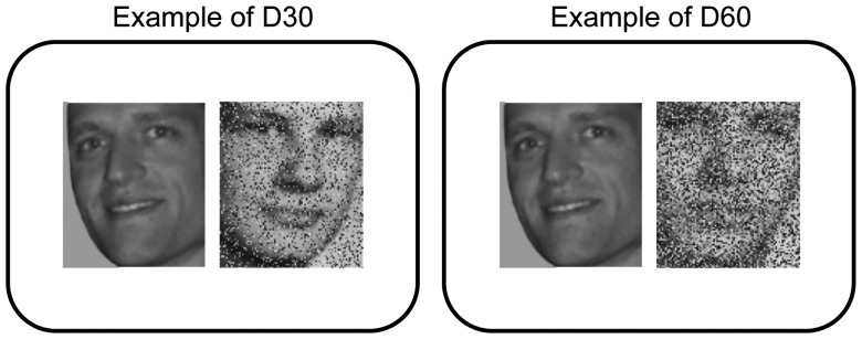
Example stimulus slides from our D30 and D60 conditions. The images on the right of each example slide are degraded by overlaying random gray values over 30% and 60% of pixels, respectively. Subjects are asked to judge (yes/no) whether the 2 images on each slide are of the same person or not.

MRI Scanning and Preprocessing

We acquired images with a Siemens Trio 3T magnet. We first obtained a T₁-weighted anatomical volume using MPRAGE (TE = 2.63 ms, TR = 2000 ms, FOV = 256 mm, slice thickness = 1 mm, axial plane) for co-registration with the functional images. T₂* functional images (TE = 30 ms, TR = 2000 ms, flip angle = 70°, FOV = 200 mm) were obtained using EPI acquisition. Each functional sequence consisted of 30 5-mm thick oblique axial slices, positioned to image the whole brain. A total of 144 volumes were collected for each functional scanning run.

Functional Data

Functional data were slice-time corrected using AFNI (http://afni.nimh.nih.gov/afni) and motion-corrected using AIR (http://bishopw.loni.ucla.edu/AIR5/) by registering all functional volumes to the 100th volume within-run. By averaging all functional volumes within a motion-corrected run, we calculated mean functional volumes. For each run, mean functional volume was registered with each subject's structural volume using rigid body transformation. After appropriate transform concatenations, we obtained a direct nonlinear transform from each initial fMRI volume into an unbiased, in-house developed “Common Template” space (see Garrett et al. 2010, 2011, 2013 for further details). We then applied FNIRT registration algorithm (in FSL) to derive a nonlinear transform between our anatomical Common Template and MNI 152_T1 provided with FSL software (www.fmrib.ox.ac.uk/fsl). Data were smoothed using a 7-mm Gaussian kernel.

We also performed various subsequent preprocessing steps intended to further reduce data artifacts and improve the predictive power of our SD_BOLD measure (see Garrett et al. 2010, 2011, 2013). We first examined our functional volumes in the Common Template space for artifacts via independent component analysis (ICA) within-run, within-person, as implemented in FSL/MELODIC (Beckmann and Smith 2004). A “training set” was obtained by manually classifying noise components (via visual inspection of MELODIC default thresholded component maps, and associated time series and Fourier spectrum) from a small set of runs (∼20) within randomly selected subjects. In general, we adopt and expand upon noise component characterization specified previously (Kelly et al. 2010). Noise components were targeted according to several key criteria: 1) Spiking (components dominated by abrupt time series spikes ∼≥6 SDs); 2) Motion (prominent edge or “ringing” effects, sometimes [but not always] accompanied by large time series spikes); 3) Susceptibility and flow artifacts (prominent air-tissue boundary or sinus activation; typically represents cardio/respiratory effects); 4) White matter (WM) and ventricle activation (another potential proxy for cardio/respiratory effects; Birn 2012); 5) Low-frequency signal drift (∼≤0.009 Hz; linear or nonlinear drift, perhaps representing scanner instabilities; see Smith et al. 1999); 6) High power in high-frequency ranges unlikely to represent neural activity (∼≥75% of total spectral power present above ∼0.13 Hz;); and 7) Spatial distribution (“spotty” or “speckled” spatial pattern that appears scattered randomly across ∼≥25% of the brain, with few if any clusters with ∼≥10 contiguous voxels [at 4 × 4 × 4 mm voxel size]). In line with these criteria, brief examples of several components we typically deem to be noise are highlighted in Supplementary Material. By default, we utilize a conservative set of rejection criteria; if manual classification decisions are difficult due to the co-occurrence of apparent “signal” and “noise” in a single component, we typically elect to keep such components. Thus, when in doubt, we do not reject. Two independent raters of noise components were utilized (one of which was D.D.G.); >90% inter-rater reliability was required before proceeding. Next, and related to Tohka et al. (2008), our manually classified “training set” was used to train a quadratic discriminant classifier to automatically separate components from all runs into artifact and nonartifact categories in those data not already manually classified (“test set”). Components identified as artifact were then regressed from corresponding fMRI runs using the FSL regfilt command.

Following ICA denoising, voxel time series were further adjusted by regressing out motion-correction parameters, and WM and cerebrospinal fluid (CSF) time series using in-house MATLAB code. For WM and CSF regression, we extracted time series from unsmoothed data within small ROIs in the corpus callosum and ventricles of the Common Template, respectively. ROIs were selected such that they were deep within each structure of interest (corpus callosum and ventricles) to avoid partial volume effects. The choice of a one 4-mm³ voxel within corpus callosum for WM and a same size voxel within one lateral ventricle for CSF was based on our experience in having excellent registration of these structures across groups and studies. Our rationale for applying these preprocessing steps following ICA denoising was simply a conservative choice intended to remove any within-subject artifacts that ICA may have missed, prior to calculating voxel variability values for each subject and task (see Data Analyses section).

Our additional preprocessing steps had dramatic effects on the predictive power of SD_BOLD in past research, effectively removing 50% of the variance still present after traditional preprocessing steps, while simultaneously doubling the predictive power of SD_BOLD (Garrett et al. 2010). Thus, calculating BOLD signal variance from relatively artifact-free BOLD time series permits the examination of what is more likely meaningful neural variability. Finally, to localize regions from our functional output, we submitted MNI coordinates to the Anatomy Toolbox (version 1.8) in SPM8, which applies probabilistic algorithms to determine the cytoarchitectonic labeling of MNI coordinates (Eickhoff et al. 2005, 2007).

Data Analyses

Reaction Time Measures

Prior to computing reaction time means and standard deviations per person, per task condition, we first set a lower bound (150 ms) for legitimate responses for each task on the basis of minimal RTs suggested by prior research (MacDonald et al. 2006; Dixon et al. 2007). We then trimmed extreme outliers relative to the rest of the sample on each task (≥4000 ms). We established final bounds for each task by dropping all trials more than 3 SDs from within-person means. The number of trials dropped across all participants and tasks was negligible (213/3780 total trials). For each task, to maintain realistic variability within the data, we then imputed missing values for outlier trials by using multiple imputation (100 imputations, fully conditional specification [iterative Markov chain Monte Carlo method]), and predictive mean matching (using subject ID, condition, and RT as predictors of interest), as implemented in SPSS 20.0 (IBM, Inc.). We then calculated mean reaction times (mean_RT) for each task condition, for each subject. Prior to calculating intraindividual measures of reaction time variability (ISD_RT), we first sought to disentangle potential practice effects from legitimate response variability. We used split-plot regression to residualize the effects of block order, trial, and all interactions from all RT trials separately for each face degradation condition. Using these residualized values, we calculated ISD_RT for each participant on each task as in previous studies (Dixon et al. 2007; Hultsch et al. 2008).

Calculation of Mean_BOLD and SD_BOLD

To calculate mean signal (mean_BOLD) for each experimental condition, we first expressed each signal value as a percent change from its respective block onset value, and then calculated a mean percent change within each block and averaged across all blocks for a given condition. To calculate SD_BOLD, we first performed a block normalization procedure to account for residual low-frequency artifacts. We normalized all blocks for each condition such that the overall 4D mean across brain and block was 100. For each voxel, we then subtracted the block mean and concatenated across all blocks. Finally, we calculated voxel standard deviations across this concatenated time series (see Garrett et al. 2010, 2011, 2013).

Partial Least Squares Analysis of Relations Between Task Difficulty and Brain Function (SD_BOLD and Mean_BOLD)

To examine multivariate relations between experimental conditions and brain function, we employed separate partial least squares (PLS) analyses (Task PLS; see McIntosh et al. 1996; Krishnan et al. 2011) using (1) SD_BOLD and (2) mean_BOLD as our brain measures. Task PLS begins by calculating a between-subject covariance matrix (COV) between experimental conditions and each voxel's signal (“signal” here refers to either SD_BOLD or to mean_BOLD, depending on the model). COV is then decomposed using singular value decomposition (SVD).

$$SV{D}_{COV}=US{V}^{\prime }$$ (1)

This decomposition produces a left singular vector of experimental condition weights (U), a right singular vector of brain voxel weights (V), and a diagonal matrix of singular values (S). Simply stated, this analysis produces orthogonal latent variables (LVs) that optimally represent relations between experimental conditions and brain voxels. Each LV contains a spatial activity pattern depicting the brain regions that show the strongest relation to task contrasts identified by the LV. Each voxel weight (in V) is proportional to the covariance between voxel measures and the task contrast. To obtain a summary measure of each participant's expression of a particular LV's spatial pattern, we calculated within-person “brain scores” by multiplying each voxel (i)'s weight (V) from each LV (j) (produced from the SVD in equation (1)) by voxel (i)'s value for person (k), and summing over all (n) brain voxels. For example, using SD_BOLD as the voxel measure, we have:

$$\sum _{i=1}^n{V}_{ij}S{D}_{\mathrm{BOLD}}ik$$ (2)

A mean_BOLD brain score for each subject was calculated as in equation (2) using data/values from a separate PLS model run.

Significance of detected relations between multivariate spatial patterns and experimental conditions was assessed using 1000 permutation tests of the singular value corresponding to each LV. A subsequent bootstrapping procedure revealed the robustness of voxel saliences across 1000 bootstrapped resamples of our data (Efron and Tibshirani 1993). By dividing each voxel's mean salience by its bootstrapped standard error, we obtained “bootstrap ratios” (BSR) as normalized estimates of robustness. We thresholded BSRs at a value of ≥3.00, which approximates a 99% confidence interval. Finally, all models were run on gray matter (GM) only, following the creation of a custom GM mask within our common template space.

Modeling Parametric Within-Subject Effects for Task Performance and Brain Function

Several standard repeated-measures general linear models were run to examine parametric effects separately for accuracy, mean_RT, ISD_RT, SD_BOLD brain scores, and mean_BOLD brain scores. First, all 5 models were run using “condition” as an independent variable, which was entered as a series of dummy codes to capture all variance attributed to parametric manipulation. Second, orthogonal linear and nonlinear trends were simultaneously fit (up to a cubic trend) to measure their relative contribution.

Modeling Relations Between SD_BOLD, Mean_BOLD, and Behavior Across Levels of Task Difficulty

In the context of parametric experimental designs, establishing clear relations between BOLD measures and behavior requires explicitly examining both between-subject effects (e.g., do higher levels of SD_BOLD coincide with higher levels of performance?) and within-subject effects (e.g., do changes in SD_BOLD across conditions covary with changes in performance?). This can be achieved through mixed modeling, in which between- and within-subject relations can be simultaneously estimated (Snijders and Bosker 1999; van de Pol and Wright 2009). We were also interested in comparing SD_BOLD and mean_BOLD in predicting task performance (accuracy, mean_RT, and ISD_RT), necessitating the simultaneous estimation of between- and within-subject effects for each brain measure. Prior to modeling, we first structured the data in person-period format, in which measurement occasions/conditions for each measure of interest were contained in a single column, with multiple rows per participant coinciding with the number of measurements taken (i.e., 7 rows per subject, one for each face degradation condition). Then, separately for accuracy, mean_RT, and ISD_RT, we fit a model of the form:

$${\text{Task performance}}_{\mathrm{ij}}={\beta }_0+{\beta }_{\mathrm{SD}\mathrm{\_}\mathrm{between}}{\overline{x}}_j+{\beta }_{\mathrm{SD}\mathrm{\_}\mathrm{within}}(x_{ij}-{\overline{x}}_j)+{\beta }_{\mathrm{Mean}\mathrm{\_}\mathrm{between}}{\overline{x}}_j+{\beta }_{\mathrm{Mean}\mathrm{\_}\mathrm{within}}(x_{ij}-{\overline{x}}_j)+e_{0ij}$$ (3)

Here, the task performance value for each face degradation condition (i) and participant (j) is modeled as a function of: 1) a model intercept (β₀); 2) the between-subjects SD_BOLD effect (${\beta }_{\mathrm{SD}\mathrm{\_}\mathrm{between}}{\overline{x}}_j$), in which ${\overline{x}}_j$ represents the subject SD_BOLD brain score average across task conditions; 3) the within-subjects SD_BOLD effect $({\beta }_{\mathrm{SD}\mathrm{\_}\mathrm{within}}(x_{ij}-{\overline{x}}_j))$, in which each condition-based SD_BOLD brain score is mean-centered within-person; 4) the between-subjects mean_BOLD effect (${\beta }_{\mathrm{mean}\mathrm{\_}\mathrm{between}}{\overline{x}}_j$), in which ${\overline{x}}_j$ represents the subject mean_BOLD brain score average across task conditions; 5) the within-subjects mean_BOLD effect $({\beta }_{\mathrm{mean}\mathrm{\_}\mathrm{within}}(x_{ij}-{\overline{x}}_j))$, in which each condition-based mean_BOLD brain score is mean-centered within-person; and 6) residual error (e_0ij). We chose compound symmetry (CS) as the covariance structure for all 3 models given that Akaike Information Criteria (AIC) fits were significantly better than the default diagonal covariance structure for 2 of the 3 model runs (P < 0.05), and required 5 fewer parameters to estimate (CS = 7 parameters). We also compared AIC levels for CS and the most bias-free available covariance structure (i.e., “unstructured” covariance, which required 33 estimated parameters for each model run). Owing to this increased number of estimated parameters and our modest sample size, models either did not converge or were not significantly better fitting than our CS models. Thus, overall, CS was a logical choice for all model runs. Finally, we did not model a random intercept because it is statistically redundant with the between-subject effects we modeled. All models were run using SPSS 20 (IBM, Inc.).

Results

Behavioral Manipulation

Using a series of repeated-measures general linear models, we first examined whether accuracy, mean reaction time (mean_RT), and intraindividual standard deviations of reaction time (ISD_RT) varied across our face degradation task conditions (face degradation levels varied from 0% to 70%; see Materials and Methods section). These models serve as a test of the success of our parametric task manipulation. All 3 behavioral measures exhibited robust effects over conditions (See Fig. 2 and Table 1 [models 1–6]). Accuracy decreased and mean_RT and ISD_RT increased over conditions; all trends were largely linear in form. Although ISD scores reached an apparent peak at D50 (see Fig. 2), no significant nonlinear trend was noted.

Figure 2.

Behavioral trends for accuracy, and reaction time means (mean_RT) and intraindividual standard deviations (ISD_RT) across face degradation conditions. Error bars represent bootstrapped 95% confidence intervals.

Table 1.

Task performance and brain measure repeated-measures models

Model	Conditions	Dependent variable	Predictor	df (num/denom)	F	P	Partial η2
1	D0–D70	Accuracy	Condition	(6, 102)	44.05	<0.0001	0.72
2	D0–D70	Accuracy	Linear	(1, 106)	255.49	<0.0001	0.71
			Quadratic	(1, 106)	7.02	0.01	0.06
3	D0–D70	MeanRT	Condition	(6, 102)	33.73	<0.0001	0.67
4	D0–D70	MeanRT	Linear	(1, 106)	204.41	<0.0001	0.66
			Quadratic	(1, 106)	1.73	0.19	0.02
5	D0–D70	ISDRT	Condition	(6, 102)	2.89	0.01	0.15
6	D0–D70	ISDRT	Linear	(1, 106)	14.08	<0.0001	0.12
			Quadratic	(1, 106)	2.63	0.11	0.02
7	Fixation–D70	SDBOLD brain score	Linear	(1, 124)	10.16	<0.01	0.08
			Quadratic	(1, 124)	20.90	<0.0001	0.14
8	Fixation–D70	MeanBOLD LV1 brain score	Linear	(1, 123)	121.89	<0.0001	0.50
			Quadratic	(1, 123)	81.89	<0.0001	0.40
			Cubic	(1, 123)	50.94	<0.0001	0.29
9	Fixation–D70	MeanBOLD LV2 brain score	Linear	(1, 123)	2.71	0.10	0.02
			Quadratic	(1, 123)	0.33	0.57	0.00
			Cubic	(1, 123)	0.22	0.64	0.00

Experimental Manipulation of Brain Signal Variability (SD_BOLD)

Next, we examined whether within-person brain signal variability levels changed across conditions. We first utilized multivariate PLS (task PLS; McIntosh et al. 1996; McIntosh and Lobaugh 2004; Krishnan et al. 2011) analysis to examine differences in signal variability across all conditions (fixation + all 7 face degradation conditions). A single robust LV resulted (singular value = 2.98; 42.29% crossblock covariance; permuted P < 0.0001); Figure 3a contains a plot of PLS “brain scores” for each subject across conditions (see Formula 2 in Materials and Methods section for details). The PLS brain pattern (see Fig. 3b) highlighted a unidirectional effect; the higher the brain score in Figure 3a, the higher the level of brain signal variability in regions noted in Figure 3b. Signal variability during fixation could not be distinguished from the D0 condition. However, there was a substantial increase in signal variability at D20 (i.e., the easiest condition that also included image noise) that gradually reduced through to D70 (which was reliably lower in variability than fixation and D0). A complementary repeated-measures test of these brain scores revealed both linear and quadratic effects (see Table 1, model 7). Regions with declining variability as difficulty increased from D20 included the inferior frontal gyrus, calcarine gyrus, and medial and lateral temporal regions. See Supplementary Table S1 for cluster maxima, MNI coordinates, peak BSRs, and cluster sizes for our standard threshold (BSR = 3.00) model.

Further, because PLS highlights relative changes in signal variability across conditions, it is important also to quantify the magnitude of within-person change in signal variability. Remarkably, the average between-subject magnitude of SD_BOLD decrease from D20 (the peak of signal variability) to D70 (the trough) was 11.2% (SD = 3.6%), with some voxels decreasing by as much as 26.4%.

Examination of mean_BOLD Effects

A task PLS analysis of mean brain signal across all conditions revealed 2 robust LVs. In clear contrast to our SD_BOLD contrast and spatial pattern, a largely “task negative” (at fixation) versus “task positive” (all other conditions) contrast resulted for LV1, accounting for the majority of variance (singular value = 25.30, crossblock covariance = 70.51%, permuted P < 0.0001); see Figure 4a for a plot of brain scores across conditions, and Figure 4b for its accompanying spatial pattern. Characteristic task negative regions (shown in blue) were more active at fixation (e.g., medial prefrontal, posterior cingulate/precuneus) than on task, whereas task positive regions (e.g., inferior frontal gyrus (p. opercularis), inferior parietal lobule, middle and dorsolateral PFC; shown in yellow/red) were more active on task than during fixation. Subsequent repeated-measures tests of LV1 brain scores revealed both linear, quadratic, and cubic effects (see Table 1, model 8).

LV2 (see Fig. 4c,d) revealed a modest contrast that largely captured subtle differences between D0, D20, and D30, and corresponded to a much sparser spatial pattern (singular value = 9.77, crossblock covariance = 10.53%, permuted P = 0.01). See Supplementary Table S2 for cluster maxima, MNI coordinates, peak BSRs, and cluster sizes for LV1 and LV2 results. Follow-up repeated-measures tests of LV2 brain scores revealed only a marginal linear trend (see Table 1, model 9).

Linking SD_BOLD and Task Performance, and Comparisons to mean_BOLD

Next, we examined whether SD_BOLD brain scores from our PLS model above (see Fig. 3a) covaried with cognitive performance across the 7 face degradation conditions using mixed modeling. To avoid conflating levels of data aggregation when linking brain and behavior in our parametric task design, we simultaneously modeled between-subject (e.g., do higher levels of SD_BOLD covary with higher levels of performance?) and within-subject (e.g., do changes in SD_BOLD across conditions covary with changes in performance?) effects in relation to 1) accuracy, 2) mean_RT, and 3) ISD_RT in 3 separate model runs. To compare the relative predictive power of SD_BOLD and mean_BOLD brain scores, we also simultaneously modeled between- and within-subject effects for mean_BOLD in each model run (from LV1, which was by far the strongest mean signal-based LV accounting for the vast majority of crossblock covariance; LV2 brain scores offered no predictive utility, all Ps > 0.25).

Our first model results (D0 through D70 conditions) indicated reliable within-person relations between SD_BOLD and accuracy and between SD_BOLD and mean_RT (i.e., within-person reductions in signal variability followed poorer accuracy and longer mean_RT within-person; see Table 2); mean_BOLD held no predictive power in any model. We also ran a second set of models using data only from D20 to D70, to test the apparently linear change seen across these conditions in both SD_BOLD (see Fig. 3a) and mean_BOLD (see Fig. 4a) brain scores. For both brain measures, this should represent their best chance of relating to notable linear changes in task performance across conditions noted in Figure 1. Model results remained similar to the D0–D70 models (i.e., SD_BOLD covaried with accuracy and mean_RT within-person; mean_BOLD had no predictive impact), although robust SD_BOLD effects were somewhat stronger in this model (see Table 2).

Further Comparison of SD_BOLD and Mean_BOLD

From our SD_BOLD and mean_BOLD models, it is clear that several statistical and spatial differences exist in the LVs that meet our resampling-based thresholds, and exist in relation to cognitive performance. We explored a more direct examination of this lack of relation (i.e., lack of robust contrast similarity and spatial overlap) between SD_BOLD and mean_BOLD brain measures by comparing all mean_BOLD voxel data (i.e., mean_BOLD-based preprocessed data for each voxel) with all SD_BOLD voxel data (i.e., SD_BOLD-based preprocessed data for each voxel) across subjects. Such an analysis should produce results unbiased by any particular SVD or by choices of explicit contrasts that could be fit. In our data, there were 14 346 voxels/subject/condition/brain measure; with 18 subjects and 8 conditions (i.e., fixation, D0, D20–D70), this provided 2 065 824 data points per brain measure for comparison. Despite massive power to overfit, and in line with our previous work (Garrett et al. 2010, 2011, 2013), there was no notable relation between the 2 brain measures across our sample (e.g., linear r = 0.07). We present these data (Fig. 5a) as a density-weighted scatter plot. Because of the number of data points examined in only 2 dimensions (2D), massive numbers of data points will overlap in a standard scatter plot, potentially disguising where the majority of the data lie within the scatter. Density-weighting utilizes the color spectrum to help visualize such high volume data.

Figure 5.

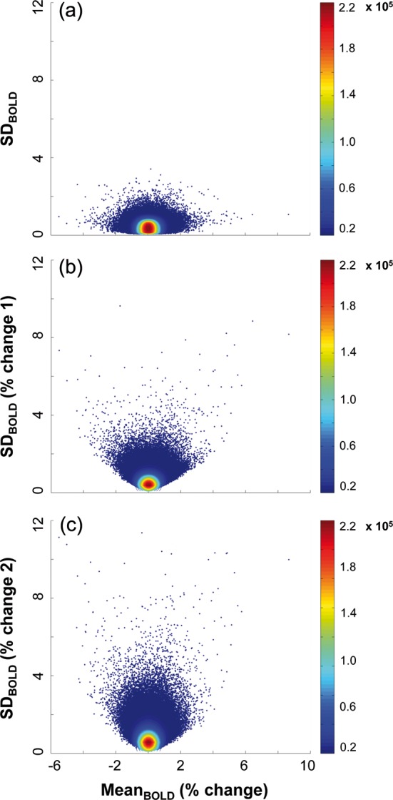
Lack of relations between mean_BOLD and 3 types of SD_BOLD. SD_BOLD in (a) represents our typical method of calculation. In (b), SD_BOLD is calculated on percent change data derived from using block means as the anchor points for trial data (i.e., “% change 1”). In (c), SD_BOLD is calculated on percent change data derived from using initial block scans as the anchor points for trial data (i.e., “% change 2”). This latter calculation on trial data is identical to what we used prior to calculating MeanBOLD (% change). In each figure, data clouds represent all voxels per subject and condition (14 346 voxels × 18 subjects × 8 conditions = 2 065 824 data points). Color bars reflect density within the data clouds.

We further examined the relation between mean_BOLD and SD_BOLD by calculating 2 additional measures of SD_BOLD. One possible source of differences between mean_BOLD and SD_BOLD measures in our data could be that our mean_BOLD measure is calculated in percent change metric (from initial block scan) and our SD_BOLD measure is not. Instead, we typically block center our trial data within-person prior to calculating SD_BOLD to account for any low-frequency drift effects (see Materials and Methods section for details). Our decision to calculate SD_BOLD in this way, rather than by using a percent change metric, theoretically allows our current and past results to be more comparable with work in which a reference condition does not exist (e.g., resting-state research). However, it is not yet known whether this choice introduces differences between mean_BOLD and SD_BOLD measures. To test this, we calculated 2 different percent change-based SD_BOLD measures: 1) using the block mean as the anchor point for block data (i.e., 100 × [block scan − block mean]/block mean), and taking the SD over all concatenated blocks for each condition; and 2) using the initial block scan as the anchor point for block data (i.e., 100× [block scan − initial block scan]/initial block scan), and taking the SD over all concatenated blocks for each condition. The first measure is the percent change equivalent of our typical SD_BOLD measure, and the second measure represents SD values calculated using exactly the same trial data calculation we use prior to computing our mean_BOLD measure (see Materials and Methods section). Regardless, relations between mean_BOLD and our 2 alternative SD_BOLD measures were equally weak (e.g., linear r = 0.05 and r = 0.04, respectively; see Fig. 5b,c for density-weighted scatter plots).

From these additional analyses, it becomes clearer why spatial and statistical differences may exist across mean_BOLD and SD_BOLD measures in our current results. Dimensionality reduction (and subsequent relations to cognitive performance) cannot at all be assumed to produce similar findings across mean_BOLD and SD_BOLD measures in our data. There were no noteworthy relations between the 2 measures across voxels, subjects, and conditions, no matter how we calculated SD_BOLD.

Discussion

In the present study, our primary focus was whether BOLD variability could be “tuned” via parametric manipulation of task difficulty, and in turn, whether task-based modulations in SD_BOLD would covary with modulations in behavioral performance. We confirmed the presence of a robust difference in signal variability across fixation and our 7 face degradation conditions. Although fixation and D0 (the easiest performance condition in which no noise was applied to any face images) exhibited similar levels of SD_BOLD, a sizable increase in SD_BOLD occurred at D20 that then decreased to D70. Interestingly, a unidirectional pattern of variability existed across brain regions, regardless of threshold level; SD_BOLD was highest at D20, and variability levels only decreased with increasing task difficulty (an average 11.32% decrease in SD_BOLD by D70) across a host of regions. Conversely, our mean_BOLD-based analysis of all conditions largely revealed a typical “task negative” (fixation-based, default mode-type activation) versus “task positive” contrast.

We then found reliable within-person covariation between lower SD_BOLD and decreasing accuracy and longer mean_RT, thus expanding previous work indicating robust relations between brain signal variability and behavioral performance (McIntosh et al. 2008; Misic et al. 2010; Garrett et al. 2011, 2013; Garrett, Samanez-Larkin et al. 2013) and further supporting the functional implications of variability levels in a variety of brain regions. Notably, our results were reliable within a sample of only healthy young adults. Most previous studies of neuroimaging-based signal variability have focused largely on more heterogeneous samples to achieve effects of interest (e.g., maturation, aging, clinical populations; McIntosh et al. 2008; Garrett et al. 2010, 2011, 2013; Misic et al. 2010; Vakorin et al. 2011; Raja Beharelle et al. 2012; Garrett, Samanez-Larkin et al. 2013). Our current results thus greatly strengthen the future applicability of signal variability measures in more homogeneous, constrained samples. However, the absence of between-subject relations between SD_BOLD and behavior in our present study indicates that, in future work, sample homogeneity may limit SD_BOLD-behavior relations primarily to the within-subject level. In any case, convergent with our first paper on BOLD variability (Garrett et al. 2010), mean_BOLD provided no unique between- or within-subject effects over and above SD_BOLD, thus further supporting the utility of future examinations of signal variability in relation to cognition.

Finally, by plotting all voxel data across subjects and conditions, we revealed largely spherical relations between mean_BOLD and SD_BOLD. Essentially, little can be learned or presumed about SD_BOLD and its corresponding spatial patterns by knowing something about mean_BOLD; they are simply very different measures of brain function.

A Closer Look at our SD_BOLD and Mean_BOLD Patterns

Although we did not explicitly measure them via a functional localizer scan, key face processing areas such as the fusiform face area and occipital face area (e.g., Kanwisher et al. 1997; Grady et al. 2000; Pessoa et al. 2002; Pitcher et al. 2011) were noted within our mean_BOLD task PLS model, which revealed that these regions were more active on task than at fixation (see Fig. 4b). However, none of the prototypical face processing areas showed robust SD_BOLD changes. The fact that typical mean-based face-processing regions did not appear in our SD_BOLD spatial pattern is not unexpected; the current results, and our previous work (Garrett et al. 2010, 2011), suggest that mean- and variability-based spatial patterns are largely nonoverlapping. Beyond face-processing regions, SD_BOLD areas that decreased with task difficulty were most prominent in the right calcarine gyrus, inferior frontal gyrus, rolandic operculum, and middle temporal gyrus. Notably, our largest cluster (calcarine gyrus peak) extended broadly into the precuneus/posterior cingulate. Increasing evidence suggests that these latter regions are not only prominent hubs of functional and structural connectivity in the human brain (Hagmann et al. 2008, 2010; Buckner et al. 2009), they can also serve as key centers for task and group related signal variability effects (Misic et al. 2010, 2011; Raja Beharelle et al. 2012), perhaps owing to the heightened information flow characteristic of such hub regions (Misic et al. 2011). In addition, our current spatial pattern of task-modulated signal variability (see Fig. 3b) was much broader than would be expected based on network centrality alone, with our highest peak regions existing outside of the precuneus/posterior cingulate. This suggests that incremental task demands can modulate brain signal variability in a variety of regions over and above what may be considered central hub-based information flow.

Interpreting Task-Related Modulations in Signal Variability

In the present study, we found that SD_BOLD increased from fixation only once noise was applied to our stimuli (D20). As the quality of incoming stimuli further degraded (toward D70), our subjects became less variable in their hemodynamic responses. First, we address points regarding the early part of the “tuning curve” (fixation, D20/30/40; see Fig. 3a). In a previous study (Garrett et al. 2013), we found similar broad-scale within-person increases in SD_BOLD from internal (fixation) to externally oriented cognitive tasks (visual tasks using gabor patch stimuli; constrained within-person at ∼80% accuracy). In that study, we argued that unidirectional increases in SD_BOLD from fixation to task could reflect: 1) greater required dynamic range on task (greater range of responses required to process varying versus static incoming stimuli); 2) stimulus uncertainty (would naturally be greater on task vs. at fixation, perhaps yielding greater response variability); and 3) “kinetic energy” (greater variability can allow the brain to transition from state to state to process differentiated and ongoing demands). In the present study, we indeed replicate this general upward trajectory from fixation to D20/30/40, supporting our previous work in younger and older adults (Garrett et al. 2013), as well as other studies (Wutte et al. 2011).

However, why would fixation not differ from D0 (an externally oriented task)? One possibility is that dynamic range, stimulus uncertainty, and/or kinetic energy are simply less present, required, or invoked when a task is too easy. Our D0 condition only required participants to judge whether 2 nondegraded faces were of the same person or not; unsurprisingly, all D0 behavioral measures were at their highest level, and accuracy was near ceiling. Previous work suggests that the level of transition from rest to task modes depends upon the difficulty of tasks administered; easier tasks do not easily force the brain out of resting state (McKiernan et al. 2003), and this plausibly could have occurred for D0 in the present study. Further, the human brain's natural affinity to process faces in their natural, upright orientation (as in the current D0 condition) may require relatively few resources (e.g., Yin 1969; Rhodes 1993; Tanaka and Farah 1993; Farah et al. 1995; Freire and Lee 2001; Mondloch et al. 2002), resulting in no fixation to D0-related change in SD_BOLD level.

With regard to the reduction in SD_BOLD from D20 to D70, there are several potential reasons this could occur. In general, greater moment-to-moment brain signal variability may serve as a proxy measure for a brain at the “edge of criticality” between various potential brain states (Ghosh et al. 2008; Deco et al. 2009, 2011), and this criticality can represent an optimal dynamic range/variability of possible responses and information transfer within networks (Shew et al. 2009, 2011; Yang et al. 2012). Computational work suggests that when variability is too low however, there is a reduced capacity for the brain to explore its dynamic range of possible brain states to converge on optimal neural responses (Ghosh et al. 2008; Deco et al. 2009, 2011; McIntosh et al. 2010). In the current study, we found that SD_BOLD decreased from D20 with increasing task difficulty, suggesting that the ability to vary between brain states across moments (insofar as signal variability serves as a proxy for such a phenomenon) modulates with even incremental changes in task demand. At any given moment, the more difficult a task, the more brain resources are engaged, leaving fewer resources available to process other potential tasks that may arise in one's environment or to transition to other brain states when required. In this way, the brain may be less able to spontaneously explore or even access its full dynamic repertoire (Ghosh et al. 2008; Deco et al. 2009, 2011; McIntosh et al. 2010) when forced to its processing limits, representing reduced signal variability from moment to moment, and potentially a compressed or constrained multistable attractor landscape (Deco and Jirsa 2012). Accordingly, in simple terms, signal variability may be analogous to the neural “degrees of freedom” available in the human brain at any given moment.

Thus, we refine our previous notion of condition-modulated signal variability (Garrett et al. 2013) as now encompassing a combination of internal vs. external cognitive demands, absolute level of cognitive demand, and finite processing resources. Future parametric work in other task domains is required to address our various points made here, and such work would be particularly informative should it include both signal variance measures and more dynamic measures of brain signal, as experimental designs allow (e.g., power-law scaling, Hurst exponents, entropy measures; McIntosh et al. 2008; He et al. 2010, 2011; Misic et al. 2010, 2011; Vakorin et al. 2011). Regardless of interpretation, SD_BOLD appears incrementally modifiable via the experimental control of targeted cognitive processes, and outweighs mean_BOLD in predicting cognitive performance. Critically, our findings highlight that signal stabilization (He 2011, 2013) and expansion (Wutte et al. 2011; Garrett et al. 2013) from fixation to task can occur in the same brain, depending on exactly what it is being asked to do (Garrett, Samanez-Larkin et al. 2013).

Supplementary Material

Supplementary material can be found at: http://www.cercor.oxfordjournals.org/

Funding

This work was supported by Canadian Institutes of Health Research grants to C.L.G. (MOP14036) and A.R.M. (MOP13026), and a JS McDonnell Foundation grant to A.R.M. C.L.G. is supported also by the Canada Research Chairs program, the Ontario Research Fund, and the Canadian Foundation for Innovation.

References

- Beckmann CF, Smith SM. Probabilistic independent component analysis for functional magnetic resonance imaging. IEEE Trans Med Imaging. 2004;23:137–152. doi: 10.1109/TMI.2003.822821. [DOI] [PubMed] [Google Scholar]
- Birn RM. The role of physiological noise in resting-state functional connectivity. Neuroimage. 2012;62:864–870. doi: 10.1016/j.neuroimage.2012.01.016. [DOI] [PubMed] [Google Scholar]
- Buckner RL, Sepulcre J, Talukdar T, Krienen FM, Liu H, Hedden T, Andrews-Hanna JR, Sperling RA, Johnson KA. Cortical hubs revealed by intrinsic functional connectivity: mapping, assessment of stability, and relation to Alzheimer's disease. J Neurosci. 2009;29:1860–1873. doi: 10.1523/JNEUROSCI.5062-08.2009. [DOI] [PMC free article] [PubMed] [Google Scholar]
- Deco G, Jirsa VK. Ongoing cortical activity at rest: criticality, multistability, and ghost attractors. J Neurosci. 2012;32:3366–3375. doi: 10.1523/JNEUROSCI.2523-11.2012. [DOI] [PMC free article] [PubMed] [Google Scholar]
- Deco G, Jirsa VK, McIntosh AR. Emerging concepts for the dynamical organization of resting-state activity in the brain. Nat Rev Neurosci. 2011;12:43–56. doi: 10.1038/nrn2961. [DOI] [PubMed] [Google Scholar]
- Deco G, Jirsa VK, McIntosh AR, Sporns O, Kotter R. Key role of coupling, delay, and noise in resting brain fluctuations. Proc Natl Acad Sci U S A. 2009;106:10302–10307. doi: 10.1073/pnas.0901831106. [DOI] [PMC free article] [PubMed] [Google Scholar]
- Dixon RA, Garrett DD, Lentz TL, MacDonald SWS, Strauss E, Hultsch DF. Neurocognitive markers of cognitive impairment: exploring the roles of speed and inconsistency. Neuropsychology. 2007;21:381–399. doi: 10.1037/0894-4105.21.3.381. [DOI] [PubMed] [Google Scholar]
- Efron B, Tibshirani R. An introduction to the bootstrap. Boca Raton, FL: Chapman & Hall/CRC; 1993. [Google Scholar]
- Eickhoff SB, Paus T, Caspers S, Grosbras MH, Evans AC, Zilles K, Amunts K. Assignment of functional activations to probabilistic cytoarchitectonic areas revisited. Neuroimage. 2007;36:511–521. doi: 10.1016/j.neuroimage.2007.03.060. [DOI] [PubMed] [Google Scholar]
- Eickhoff SB, Stephan KE, Mohlberg H, Grefkes C, Fink GR, Amunts K, Zilles K. A new SPM toolbox for combining probabilistic cytoarchitectonic maps and functional imaging data. Neuroimage. 2005;25:1325–1335. doi: 10.1016/j.neuroimage.2004.12.034. [DOI] [PubMed] [Google Scholar]
- Faisal AA, Selen LP, Wolpert DM. Noise in the nervous system. Nat Rev Neurosci. 2008;9:292–303. doi: 10.1038/nrn2258. [DOI] [PMC free article] [PubMed] [Google Scholar]
- Farah MJ, Tanaka JW, Drain HM. What causes the face inversion effect? J Exp Psychol Hum Percept Perform. 1995;21:628–634. doi: 10.1037//0096-1523.21.3.628. [DOI] [PubMed] [Google Scholar]
- Freire A, Lee K. Face recognition in 4- to 7-year-olds: processing of configural, featural, and paraphernalia information. J Exp Child Psychol. 2001;80:347–371. doi: 10.1006/jecp.2001.2639. [DOI] [PubMed] [Google Scholar]
- Garrett DD, Kovacevic N, McIntosh AR, Grady CL. Blood oxygen level-dependent signal variability is more than just noise. J Neurosci. 2010;30:4914–4921. doi: 10.1523/JNEUROSCI.5166-09.2010. [DOI] [PMC free article] [PubMed] [Google Scholar]
- Garrett DD, Kovacevic N, McIntosh AR, Grady CL. The importance of being variable. J Neurosci. 2011;31:4496–4503. doi: 10.1523/JNEUROSCI.5641-10.2011. [DOI] [PMC free article] [PubMed] [Google Scholar]
- Garrett DD, Kovacevic N, McIntosh AR, Grady CL. The modulation of BOLD variability between cognitive states varies by age and processing speed. Cereb Cortex. 2013;23:684–693. doi: 10.1093/cercor/bhs055. [DOI] [PMC free article] [PubMed] [Google Scholar]
- Garrett DD, Samanez-Larkin GR, Macdonald SW, Lindenberger U, McIntosh AR, Grady CL. Moment-to-moment brain signal variability: a next frontier in human brain mapping? Neurosci Biobehav Rev. 2013;37:610–624. doi: 10.1016/j.neubiorev.2013.02.015. [DOI] [PMC free article] [PubMed] [Google Scholar]
- Ghosh A, Rho Y, McIntosh AR, Kotter R, Jirsa VK. Noise during rest enables the exploration of the brain's dynamic repertoire. PLoS Comput Biol. 2008;4:e1000196. doi: 10.1371/journal.pcbi.1000196. [DOI] [PMC free article] [PubMed] [Google Scholar]
- Grady CL, McIntosh AR, Horwitz B, Rapoport SI. Age-related changes in the neural correlates of degraded and nondegraded face processing. Cogn Neuropsychol. 2000;17:165–186. doi: 10.1080/026432900380553. [DOI] [PubMed] [Google Scholar]
- Hagmann P, Cammoun L, Gigandet X, Meuli R, Honey CJ, Wedeen VJ, Sporns O. Mapping the structural core of human cerebral cortex. PLoS Biol. 2008;6:e159. doi: 10.1371/journal.pbio.0060159. [DOI] [PMC free article] [PubMed] [Google Scholar]
- Hagmann P, Sporns O, Madan N, Cammoun L, Pienaar R, Wedeen VJ, Meuli R, Thiran JP, Grant PE. White matter maturation reshapes structural connectivity in the late developing human brain. Proc Natl Acad Sci U S A. 2010;107:19067–19072. doi: 10.1073/pnas.1009073107. [DOI] [PMC free article] [PubMed] [Google Scholar]
- He BJ. Scale-free properties of the functional magnetic resonance imaging signal during rest and task. J Neurosci. 2011;31:13786–13795. doi: 10.1523/JNEUROSCI.2111-11.2011. [DOI] [PMC free article] [PubMed] [Google Scholar]
- He BJ. Spontaneous and task-evoked brain activity negatively interact. J Neurosci. 2013;33:4672–4682. doi: 10.1523/JNEUROSCI.2922-12.2013. [DOI] [PMC free article] [PubMed] [Google Scholar]
- He BJ, Zempel JM, Snyder AZ, Raichle ME. The temporal structures and functional significance of scale-free brain activity. Neuron. 2010;66:353–369. doi: 10.1016/j.neuron.2010.04.020. [DOI] [PMC free article] [PubMed] [Google Scholar]
- Hultsch DF, Strauss E, Hunter MA, MacDonald SWS. Intraindividual variability, cognition, and aging. In: Craik FI, Salthouse TA, editors. The handbook of aging and cognition. New York: Psychology Press; 2008. pp. 491–556. [Google Scholar]
- Kanwisher N, McDermott J, Chun MM. The fusiform face area: a module in human extrastriate cortex specialized for face perception. J Neurosci. 1997;17:4302–4311. doi: 10.1523/JNEUROSCI.17-11-04302.1997. [DOI] [PMC free article] [PubMed] [Google Scholar]
- Kelly RE, Jr, Alexopoulos GS, Wang Z, Gunning FM, Murphy CF, Morimoto SS, Kanellopoulos D, Jia Z, Lim KO, Hoptman MJ. Visual inspection of independent components: defining a procedure for artifact removal from fMRI data. J Neurosci Methods. 2010;189:233–245. doi: 10.1016/j.jneumeth.2010.03.028. [DOI] [PMC free article] [PubMed] [Google Scholar]
- Krishnan A, Williams LJ, McIntosh AR, Abdi H. Partial Least Squares (PLS) methods for neuroimaging: a tutorial and review. Neuroimage. 2011;15:455–475. doi: 10.1016/j.neuroimage.2010.07.034. [DOI] [PubMed] [Google Scholar]
- Li S-C, Van Oertzen T, Lindenberger U. A neurocomputational model of stochastic resonance and aging. Neurocomputing. 2006;69:1553–1560. [Google Scholar]
- MacDonald SWS, Hultsch DF, Bunce D. Intraindividual variability in vigilance performance: does degrading visual stimuli mimic age-related "neural noise?". J Clin Exp Neuropsychol. 2006;28:655–675. doi: 10.1080/13803390590954245. [DOI] [PubMed] [Google Scholar]
- McIntosh AR, Bookstein FL, Haxby JV, Grady CL. Spatial pattern analysis of functional brain images using partial least squares. Neuroimage. 1996;3:143–157. doi: 10.1006/nimg.1996.0016. [DOI] [PubMed] [Google Scholar]
- McIntosh AR, Kovacevic N, Itier RJ. Increased brain signal variability accompanies lower behavioral variability in development. PLoS Comput Biol. 2008;4:e1000106. doi: 10.1371/journal.pcbi.1000106. [DOI] [PMC free article] [PubMed] [Google Scholar]
- McIntosh AR, Kovacevic N, Lippe S, Garrett DD, Grady CL, Jirsa V. The development of a noisy brain. Arch Ital Biol. 2010;148:323–337. [PubMed] [Google Scholar]
- McIntosh AR, Lobaugh NJ. Partial least squares analysis of neuroimaging data: applications and advances. Neuroimage. 2004;23(Suppl 1):S250–S263. doi: 10.1016/j.neuroimage.2004.07.020. [DOI] [PubMed] [Google Scholar]
- McKiernan KA, Kaufman JN, Kucera-Thompson J, Binder JR. A parametric manipulation of factors affecting task-induced deactivation in functional neuroimaging. J Cogn Neurosci. 2003;15:394–408. doi: 10.1162/089892903321593117. [DOI] [PubMed] [Google Scholar]
- Misic B, Mills T, Taylor MJ, McIntosh AR. Brain noise is task dependent and region specific. J Neurophysiol. 2010;104:2667–2676. doi: 10.1152/jn.00648.2010. [DOI] [PubMed] [Google Scholar]
- Misic B, Vakorin VA, Paus T, McIntosh AR. Functional embedding predicts the variability of neural activity. Front Syst Neurosci. 2011;5:90. doi: 10.3389/fnsys.2011.00090. [DOI] [PMC free article] [PubMed] [Google Scholar]
- Mondloch CJ, Le Grand R, Maurer D. Configural face processing develops more slowly than featural face processing. Perception. 2002;31:553–566. doi: 10.1068/p3339. [DOI] [PubMed] [Google Scholar]
- Pessoa L, McKenna M, Gutierrez E, Ungerleider LG. Neural processing of emotional faces requires attention. Proc Natl Acad Sci U S A. 2002;99:11458–11463. doi: 10.1073/pnas.172403899. [DOI] [PMC free article] [PubMed] [Google Scholar]
- Pitcher D, Walsh V, Duchaine B. The role of the occipital face area in the cortical face perception network. Exp Brain Res. 2011;209:481–493. doi: 10.1007/s00221-011-2579-1. [DOI] [PubMed] [Google Scholar]
- Raja Beharelle A, Kovacevic N, McIntosh AR, Levine B. Brain signal variability relates to stability of behavior after recovery from diffuse brain injury. Neuroimage. 2012;60:1528–1537. doi: 10.1016/j.neuroimage.2012.01.037. [DOI] [PMC free article] [PubMed] [Google Scholar]
- Rhodes G. Configural coding, expertise, and the right hemisphere advantage for face recognition. Brain Cogn. 1993;22:19–41. doi: 10.1006/brcg.1993.1022. [DOI] [PubMed] [Google Scholar]
- Shew WL, Yang H, Petermann T, Roy R, Plenz D. Neuronal avalanches imply maximum dynamic range in cortical networks at criticality. J Neurosci. 2009;29:15595–15600. doi: 10.1523/JNEUROSCI.3864-09.2009. [DOI] [PMC free article] [PubMed] [Google Scholar]
- Shew WL, Yang H, Yu S, Roy R, Plenz D. Information capacity and transmission are maximized in balanced cortical networks with neuronal avalanches. J Neurosci. 2011;31:55–63. doi: 10.1523/JNEUROSCI.4637-10.2011. [DOI] [PMC free article] [PubMed] [Google Scholar]
- Smith AM, Lewis BK, Ruttimann UE, Ye FQ, Sinnwell TM, Yang Y, Duyn JH, Frank JA. Investigation of low frequency drift in fMRI signal. Neuroimage. 1999;9:526–533. doi: 10.1006/nimg.1999.0435. [DOI] [PubMed] [Google Scholar]
- Snijders T, Bosker RJ. Multievel analysis: an introduction to basic and advanced multilevel modeling. London: SAGE Publications. 1999 [Google Scholar]
- Tanaka JW, Farah MJ. Parts and wholes in face recognition. Q J Exp Psychol A. 1993;46:225–245. doi: 10.1080/14640749308401045. [DOI] [PubMed] [Google Scholar]
- Tohka J, Foerde K, Aron AR, Tom SM, Toga AW, Poldrack RA. Automatic independent component labeling for artifact removal in fMRI. NeuroImage. 2008;39:1227–1245. doi: 10.1016/j.neuroimage.2007.10.013. [DOI] [PMC free article] [PubMed] [Google Scholar]
- Vakorin VA, Lippe S, McIntosh AR. Variability of brain signals processed locally transforms into higher connectivity with brain development. J Neurosci. 2011;31:6405–6413. doi: 10.1523/JNEUROSCI.3153-10.2011. [DOI] [PMC free article] [PubMed] [Google Scholar]
- van de Pol M, Wright J. A simple method for distinguishing within-versus between-subject effects using mixed models. Animal Behaviour. 2009;77:753–758. [Google Scholar]
- Wutte MG, Smith MT, Flanagin VL, Wolbers T. Physiological signal variability in hMT+ reflects performance on a direction discrimination task. Front Psychol. 2011;2:185. doi: 10.3389/fpsyg.2011.00185. [DOI] [PMC free article] [PubMed] [Google Scholar]
- Yang H, Shew WL, Roy R, Plenz D. Maximal variability of phase synchrony in cortical networks with neuronal avalanches. J Neurosci. 2012;32:1061–1072. doi: 10.1523/JNEUROSCI.2771-11.2012. [DOI] [PMC free article] [PubMed] [Google Scholar]
- Yin R. Looking at upside-down faces. J Exp Psychol. 1969;81:141–145. [Google Scholar]
Associated Data
This section collects any data citations, data availability statements, or supplementary materials included in this article.