Effect of lesions on the dynamics of DNA on the picosecond and nanosecond timescales using a polarity sensitive probe

Abstract

This paper explores the effects of structural modifications on the fast dynamics of DNA and the ability of time-resolved Stokes shift spectroscopy to measure those changes. The time-resolved Stokes shift of a synthetic coumarin base-pair replacement within an oligomer is measured between 40 ps and 40 ns. Comparisons are made between 17mers without modification, with a deleted base near the coumarin and with the coumarin placed near the end of the oligomer. The deletion of a next-to-nearest-neighbor base pair does not change the subnanosecond dynamics, but does cause an additional motion with a time constant of ∼20 ns. A candidate for this motion is the flipping of the abasic sugar out of the helix and the concomitant intrusion of water into the interior of the helix. A nearby chain end causes little change in the dynamics after 1 ns but leads to a reduction in the amplitude of the dynamics between 40 ps and 1 ns. We suggest that at the chain end, where DNA on one side of the probe has been replaced by water, the charge- stabilizing dynamics have the same overall amplitude, but that much of the relaxation occurs before the start of the measurement time window.

INTRODUCTION

Although the time-averaged structure of DNA is understood at a high level, thermal fluctuations about that average structure have been more difficult to measure. We recently introduced a new method for studying DNA dynamics, time-resolved Stokes shift (TRSS) spectroscopy (1–4). Studies using this method have established general features of DNA dynamics that distinguish it from other molecular systems. These include a large range of motion within the picosecond and nanosecond timescales (2), unusual logarithmic kinetics (3) and sensitivity to counter-ion binding (4). This paper explores the range of variation within the family of DNA structures. Specifically, we compare the dynamics of a normal DNA sequence with those of two models of damaged DNA: an abasic site and a helix terminus. Because these comparisons are looking for small effects, the reproducibility of the TRSS method is tested and improvements in the analysis method are made.

The fluorescence of the native DNA bases decays within a few picoseconds (5) and so is not useful in a TRSS experiment. We must introduce a long-lived solvatochromic fluorophore into the DNA structure to act as a probe for the nearby dynamics. In the current experiments, we use a coumarin-102 deoxyriboside (6) in the synthesis of the oligonucleotides (Fig. 1). When paired with a tetrahydrofuran abasic site analog on the complementary strand, molecular modeling indicates that the coumarin group occupies the position of a base pair within the DNA helix and only slightly alters the DNA structure (2). This conclusion is supported by circular dichroism spectra showing B-form helices and by optical spectra and quenching studies that show that the coumarin is solvent inaccessible. Furthermore, the oligonucleotides remain biologically active for binding and cleavage by 5′-apurinic/apyrimidinic endonuclease (APE1), albeit with moderately reduced efficiency relative to strands with native bases (M.Wyatt, personal communication). Thus the coumarin is well positioned to sense the conditions typical of the interior of DNA.

Figure 1.

Structure of the fluorescent probe and its complementary abasic site. The probe is large enough to fill the entire space left by removing a base pair.

The optical spectra of the coumarin chromophore are sensitive to the polarity of the coumarin’s surroundings (7,8). Upon optical excitation, there is an intramolecular charge transfer within the coumarin that increases its dipole moment. The electric field from this dipole extends into the material surrounding the coumarin and exerts a force on any group with a full or partial charge. These groups then move at a rate determined by the intrinsic dynamics of the system. As they move, they lower the energy of the coumarin by changing the local electric field at the coumarin and thereby stabilize the excited state dipole. As the energy of the coumarin excited state is reduced, its fluorescence shifts to lower frequency. The TRSS experiment consists of monitoring the shift of this emission spectrum as a function of time after excitation (9,10).

The time-dependent spectral shift is a direct measure of the response of the various components of the DNA to the photoinduced dipole on the coumarin. Although the motion of the DNA is driven by an artificial source, the induced dipole moment, the rate of response is determined by the intrinsic dynamics of the DNA. The fluctuation–dissipation theorem guarantees that the dynamics seen in the TRSS experiment are the same ones that occur due to thermal fluctuations in the unperturbed system (11).

TRSS experiments have a number of features that provide a perspective on DNA dynamics that is distinctly different from the perspective provided by other techniques. First, TRSS experiments measure motion on fast timescales, from 40 ns to 40 ps in the current experiments, with extension to <100 fs possible with existing techniques. By comparison, NMR (12–14) and EPR (15) measurements are sensitive to longer-timescale motion, but lose sensitivity as motions move into the subnanosecond region. Changes in fluorescence quantum yield may be caused by fast motions, but the quantum yield measurements do not resolve those motions in time (16). Fluorescence anisotropy measurements extend into the picosecond time range (17,18), but measure motion relative to the laboratory reference frame (as NMR and EPR also do). As a result, they are most sensitive to large-amplitude motions, such as long-range bending and twisting of the helix. In contrast, the TRSS experiment is sensitive to motion relative to the molecular frame and over the distance of electrostatic interactions. These features make TRSS measurements most sensitive to motion of molecule-sized groups within the DNA and to other molecules, such as water and ions, in the local environment.

Other techniques, such as X-ray crystallography or NMR, provide accurate pictures in terms of the Cartesian coordinates. In contrast, the TRSS experiment is directly sensitive to a chemically relevant parameter, the local polarity. Polarity is a well known concept that characterizes the total ability of a solvent to stabilize charge (19,20). Polarity encompasses a number of specific mechanisms, including dielectric relaxation, electronic polarizability and solvent quadrupole reorientation (21), that all contribute to the same total chemical effect. In the currently relevant case of a dipolar charge distribution, polarity and the TRSS experiment measure the stabilizing electric field that the environment creates at the induced dipole.

Regardless of the specific mechanism, polarity involves the reorganization of the local environment of a charge or charge distribution to lower its energy. Thus the polarity is characterized by a rate of reorganization in addition to the total energy of stabilization at equilibrium. The rate of reorganization is most famously known to govern the rate of fast electron transfer (22), but it also affects chemical rates, when the charge distribution changes in the transition state (23,24).

The current experiments measure the reorganization of the DNA structure to stabilize a dipole moment within its interior. This reorganization is the collective effect from a variety of groups within the DNA and the nearby solvent, with the importance of each group weighted by its effectiveness in changing the electric field at the probe. The positions and orientations of nearby water molecules and ions as well as phosphate charges and base heteroatoms are all likely contributors to the TRSS measurement. The individual contribution of any of these groups is not immediately obvious without further analysis. Nevertheless, it is the total contribution of all these groups that directly affects chemical interactions, and it is this total that is measured by the TRSS experiment. Although TRSS measurements do not give a visual picture of the motion of atoms in Cartesian space, they do give a chemical picture of the DNA as sensed by chemical interactions.

TRSS experiments have been extensively used to study the dynamics of simple liquids, which in this context are often called ‘solvation dynamics’ (9,24–26). Other techniques, such as three-pulse-echo peak shifts (27) and 2D electronic spectroscopy (28), have been introduced as alternative methods for measuring solvation dynamics in liquids. In the last few years, at least 10 groups have extended these solvation experiments to proteins (29–38).

In comparison, relatively little has been done with DNA. Computer simulations have long suggested that there are substantial subnanosecond fluctuation in the DNA structure (39–41), although fluctuations in the local electric field have not been specifically examined. There have been a few reports of steady state Stokes shifts of dyes bound in the grooves of DNA (42–44). Our previous papers demonstrated the feasibility of TRSS measurements in the interior of DNA (1–4). They also showed that the dynamics observed in DNA are characteristically different from those observed in other condensed phase systems. The rates are broadly distributed over at least three decades in time. Rather than normal kinetics that are described by an exponential e^–kt or as a sum of exponentials, the TRSS dynamics of DNA are well described by logarithmic kinetics, log(t/t₀). Pal et al. (45) have made TRSS measurements on a groove-bound dye. Because their measurements were over a different time range, it is not possible to say if they see the same phenomena that we have reported.

Rather than trying to explain the origin of the unusual dynamics in DNA, this paper looks at whether changes in the DNA structure can alter those dynamics. It is conceivable that the TRSS dynamics of DNA are very different from those of typical liquids, but that all DNA structures would have essentially the same dynamics. In fact, we find that representative lesions in the DNA structure produce clear and qualitative changes in the TRSS signal. Thus the TRSS experiment has potential for characterizing the dynamical changes induced by lesions and for assessing their possible role in the biological recognition of DNA damage (46,47).

Three oligonucleotide sequences were used in this work (Table 1): sequence 1 representing ‘normal’ DNA, sequence 2 containing an extra abasic site and sequence 3 showing the effects of double-strand cleavage. The abasic lesion is an apyrimidinic site in which an entire base is deleted from the normal DNA structure (‘abasic’ sequence 2). Spontaneous hydrolysis of the glycosidic bond to create an abasic site is a common form of spontaneous damage to DNA (48–50). Abasic sites also appear as intermediates in the base-excision repair of other types of lesion (51). In the complex with the AP endonuclease that initiates the repair sequence, the DNA is sharply bent, leading to the hypothesis that increased flexibility of the abasic site is important in its recognition by the endonuclease (46,47).

Table 1. Oligonucleotide sequences used in this study.

Designation	Sequence
1 (‘normal’)	5′-GCATGCGC*CGCGTACG-3′
	3′-CGTACGCGφGCGCATGC-5′
2 (‘abasic’)	5′-GCATGCGC*CGCGTACG-3′
	3′-CGTACGφGφGCGCATGC-5′
3 (‘chain-end’)	5′-C*CGCGTACGGCATGCG-3′
	3′-GφGCGCATGCCGTACGC-5′

The coumarin-102 C-deoxyriboside probe is represented by * and an abasic site analog is represented by φ.

The second lesion studied is the abrupt termination of the DNA helix (‘chain-end’ sequence 3), which is commonly believed to induce ‘fraying’ at the end of the helix. The termination of the helix can be used as an extreme model of other major disruptions to the helical structure such as strand breaks, helix openings or junctions. The complete termination of the helix provides an upper bound on the range of dynamic perturbations to be expected in these more common structures.

Before looking at the effects of these two lesions, it is important to accurately characterize the behavior of normal DNA. In particular, the accuracy and reproducibility of the TRSS measurements should be known, so that physically significant changes can be distinguished from experimental noise. In the Materials and Methods section, we describe a new method for extracting a Stokes shift from time-resolved spectra with improved accuracy and reproducibility. This method is robust toward experimental noise, but accommodates the wide range of spectral shapes found in DNA.

MATERIALS AND METHODS

Sample preparation

Coumarin-102 C-deoxyriboside was synthesized as described by Coleman and Madaras (6). Oligonucleotides containing the coumarin-102 C-deoxyriboside were synthesized by standard procedures (2). Complementary strands were either synthesized or obtained commercially.

The oligonucleotides were dissolved in sodium phosphate buffer (pH 7.2, 100 mM) at a concentration of 0.1 mM in nucleotides (6 µM in coumarin). At the excitation wavelength of 395 nm, the samples had an absorbance of 0.03 through the 5 mm long region from which fluorescence was collected. Reabsorption of the fluorescence within the 3 × 3 mm cross-section of the cell was negligible.

Circular dichroism spectra of the oligomers indicate B-form helical DNA. The sample temperature in the TRSS experiment was maintained at 15°C by thermal contact between the sample cell and an actively regulated sample block. Melting experiments indicate complete hybridization of each of the sequences at this temperature, despite the disruptions in the DNA structure.

Steady state spectroscopy

Room temperature steady state emission spectra (Fig. 2A) were excited at 385 nm with excitation and collection bandpasses of 8 and 4 nm, respectively. The emission spectra were corrected for instrumental sensitivity to radiometric intensity units I(λ) (W/nm) (52). Excitation spectra were detected at 525 nm with emission and excitation bandpasses of 4 and 8 nm, respectively (Fig. 2A). All spectroscopy was performed with magic-angle polarization.

Figure 2.

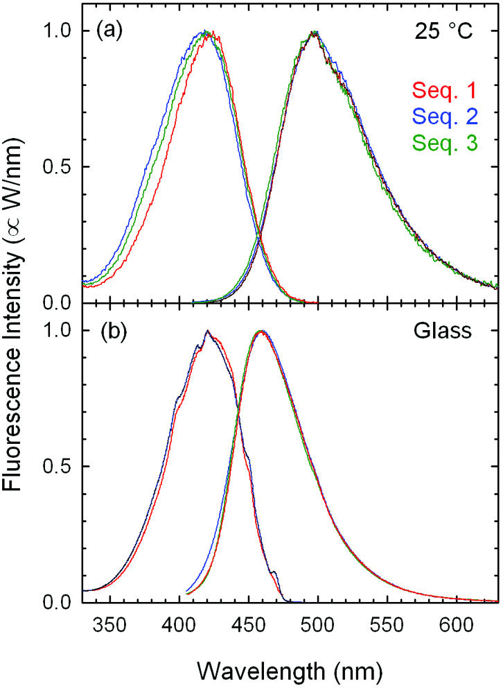
Excitation (left) and emission (right) spectra for three DNA oligonucleotide sequences (Table 1) that incorporate a coumarin-102 fluorophore: (A) at room temperature in aqueous buffer; (B) at 195 K in a buffer– glycerol glass (1:3). The increased red-shift of the emission in (A) reflects the magnitude of diffusive relaxation in the DNA. The sequence 3 spectra are partially obscured by the sequence 1 spectra in (B).

Spectra in a rigid glassy matrix (Fig. 2B) were obtained under the same conditions from oligonucleotides in a 3:1 solution of glycerol and the sodium phosphate buffer (pH 7.2, 100 mM). The samples were frozen to a glass using a bath of dry ice in acetone (195 K).

Subsequent steady state and time-resolved spectra are presented and analyzed as susceptibility χ” versus frequency ν. This format has a number of advantages for the quantitative analysis of spectra. Unlike the wavelength, the frequency is directly related to the energy of a transition, and thus shifts along a frequency axis are directly proportional to changes in molecular energy. Susceptibility spectra are more directly related to theoretical expressions for spectral line shapes than intensities are (53–55). It is in the form of susceptibility spectra that absorption and emission display mirror symmetry. The area under a susceptibility spectrum also remains proportional to population, even as the spectrum shifts in frequency.

The conversion from intensity to susceptibility is detailed in the Supplementary Material. Whether analyzed as intensities or susceptibilities, the same qualitative trends with time and comparisons between samples still hold. The analysis here is conducted with susceptibilities to facilitate future comparisons with theory and other experiments (e.g. transient absorption measurements) that are in progress.

Emission and excitation spectra were also collected from coumarin 102 (without DNA) in ethanol glass at 77 K. Emission spectra were excited at 400 nm and excitation spectra were detected at 480 nm.

Time-resolved spectroscopy

The time-resolved measurements were made using standard time-correlated single-photon counting techniques (56–58). Subpicosecond pulses were generated at 8 MHz from a mode-locked Ti:sapphire laser with an external acousto-optic pulse picker. Excitation pulses were produced at 395 nm by second-harmonic generation in a 1 mm β-barium borate (BBO) crystal. Fluorescence was collected through a 20 mm diameter Glan-laser polarizer set at the magic angle (54.7°) to eliminate any rotational effects. A subtractive double monochromator with a bandpass of 2 nm selected the fluorescence wavelength. The fluorescence photons were detected by a microchannel plate detector and timed relative to the exciting laser pulse with standard electronics.

The instrument response function was measured from a scattering solution prior to each fluorescence decay measurement. It had a typical full width at half-maximum (FWHM) of 50 ps and drifted by no more than one channel in any experiment.

Fluorescence decay measurements were made at 10 equally spaced wavelengths between 420 and 600 nm. A total of 4 × 10⁷ counts were collected in each decay, except at 420 and 600 nm where only 4 × 10⁶ counts were collected due to the low signal level. Sample datasets are shown in Figure 3.

Figure 3.

Examples of time-resolved fluorescence decay data at three collection wavelengths for sequence 1. In order of increasing decay time, the wavelengths are 460, 500 and 580 nm, corresponding to the high-frequency side, peak and low-frequency side of the steady state emission spectrum, respectively (see Fig. 2A). The difference between the decay curves is due to a dynamic Stokes shift.

Time-resolved spectra were reconstructed by standard methods (7). Each fluorescence decay curve was first fitted to an empirical fitting function using iterative reconvolution. The fitting function consisted of a sum of two to five exponentials plus an overall background and an instrument-response time shift. After fitting, the amplitude of the fitting function for each wavelength was adjusted to match its integral to the relative intensity of the steady state emission spectrum at the same wavelength. Time-resolved spectra were obtained by evaluating the fitting functions at the desired time. Examples are shown in Figures 4 and 5.

Figure 4.

An example of a reconstructed emission spectrum from sequence 1 at 500 ps (points). A log-normal function fitted to the peak (dashed curve, equation 1) does not fit the high-frequency edge of the spectrum well. A cubic-spline interpolation (solid curve, see text) was used in the current analysis.

Figure 5.

Examples of reconstructed emission spectra of sequence 1 at various times: up-triangles, 40 ps; squares, 400 ps; down-triangles, 4 ns; circles, 40 ns. The spectra are normalized to equal area.

Spectral interpolation with cubic splines

The spectra that result from spectral reconstruction are sparse in frequency (Figs 4 and 5). These points must be interpolated to extract the peak or mean frequency accurately. The standard method has been to fit the points to a log-normal function (59):

where the amplitude A, center frequency ν_p, width w and asymmetry γ are adjustable parameters. This is a purely empirical function, but it has proven to be useful in the context of solvation dynamics in liquids. Because four parameters are used to fit a dataset of 10 points, this procedure is relatively robust toward experimental error in individual points.

In the standard theory of TRSS spectroscopy, the emission spectrum is predicted to shift with time, but not to change shape (55). In experiments in simple liquids, there are some changes in the shape of the emission spectrum with time (60). However, the changes are usually small enough that they can be accommodated by changes in the width and asymmetry parameters of the log-normal function. In general, these changes in emission spectral shape have been ignored. In our earlier studies in DNA, we also used log-normal fits to extract a mean frequency and ignored changes in the width and shape of the emission spectra (2,3).

Two factors have led us to develop a new approach in the current studies. First, spectral shape changes can be quite large in DNA and are physically significant. This characteristic of DNA is the subject of a separate paper, in which we conclude that the spectral shape changes are related to counter-ions binding to the DNA (4). Thus the reconstructed spectrum needs to accurately represent all the features of the spectral shape, not just its peak position. Secondly, as we seek to make more subtle comparisons between different DNA structures, the errors that are overlooked in the standard analysis become comparable to the effects that we are seeking. Figure 4 shows an example of a log-normal fit to a time-resolved spectrum in DNA. It fits the low-frequency and peak regions, but not the high-frequency wing. For high accuracy work, this function is not an adequate representation of the spectrum.

We adopt a new analysis procedure for these spectra based on cubic-spline interpolation of the data points (61). Cubic spines are an interpolation, not a fit, in the sense that the resulting curve hits each data point exactly. A cubic spline does not rely on any prior assumptions about the spectral shape other than smoothness. Thus a cubic-spline interpolation can reproduce an arbitrary spectral shape, but does not have the data-averaging effect of a log-normal fit.

The biggest problem with this approach is extrapolating the tails of the spectra. We noted that the high- and low-frequency tails of the steady state emission spectra are exponential. Inspired by this fact, we interpolated between our spectral points with a cubic spline on a semilogarithmic plot of the time-resolved spectrum. To extrapolate the tails of the spectra, we use a linear term on the semilogarithmic plot, i.e. the tails are continued as exponentials. On the high-frequency side, the extrapolation is taken from the slope of the cubic spline at the highest frequency data point. Because the data on the high-frequency side of the spectra extend to low values of the susceptibility, the area under the extrapolation on this side is small and this simple procedure is adequate.

At low frequencies, data quality is limited by the reduced sensitivity of the detector. At the same time, the frequency corrections to the data emphasize this portion of the spectrum. Using the same extrapolation procedure on this side of the spectrum gave erratic results that were very sensitive to small errors in the last two data points. First moments extracted from the resulting spectra had modest but significant errors. For example, the spectral shapes shown in Figure 6 (discussed below) were not correctly overlapped by this procedure. The reproducibility of the measurement at long and short times was also poorer than in our final analysis (see Fig. 8 below).

Figure 6.

Comparison of spectral shapes in the three DNA samples at several times. The spectra are normalized by their area ω₀ and shifted by their mean frequency ω₁. The spectral shape changes with time, but all the sequences have the same shape at a given time. Data points: normal sequence 1, circles; abasic sequence 2, triangles; chain-end sequence 3, squares. Curves: solid, average interpolated time-resolved spectrum; dashed, spectrum of sequence 1 in a glass repeated at each time. Spectra for each time have been offset vertically.

Figure 8.

Comparison between two TRSS datasets for sequence 1 (blue lines). The averaged data (red circles) are fitted with a logarithmic time dependence (black line, equation 5). Errors increase at both long and short times. The dashed lines show the reported time range (40 ps to 40 ns).

A comparison of steady state glass spectra and time-resolved spectra at different times and in different samples suggests that the shape of the low-frequency side of the spectra does not change. Therefore we measured the exponential slope of the low-frequency side of the steady state glass spectra and used this value to extrapolate the low-frequency side of the time-resolved spectra. The slope in the glass was very similar for all of the sequences, so a common average value was used to extrapolate all the time-resolved spectra. This procedure has a combination of flexibility in shape and robustness to experimental errors. Figure 4 shows an example of the final interpolation/extrapolation and demonstrates the improvement over the log-normal fit.

Spectral position characterized by first moment

Figure 5 shows examples of interpolated spectra in DNA across the observed time range. Because the shape of the spectrum is changing, the best method of quantifying the time-dependent shift is uncertain. For example, the time dependence of the peak frequency, the half-intensity point on the low-frequency side and the half-intensity point on the high-frequency side are all qualitatively similar, but quantitatively different.

In this paper, we characterize the Stokes shift through the mean frequency or first moment ω₁ of the susceptibility spectrum χ”(ν)

In each case, the integral is applied to the spectrum after interpolation and extrapolation as described above.

Compared with other measures of the spectral shift, the mean frequency has several advantages. The shift in the mean frequency can be unambiguously interpreted as the drop in the average energy of the ensemble of DNA molecules with time. Moreover, the mean frequency makes use of all the available data points, whereas other measures, such as the peak frequency, rely heavily on only a few points.

Finally, the shift of the mean frequency is additive for independent processes. If the spectrum is broadened or shifted by two independent processes, the full spectrum χ”(ν) is the convolution of the contributions from each process χ_I”(ν) and χ_II”(ν):

In this case, the mean frequency shifts are additive:

ω₁(t) = ω_1,I(t) + ω_1,II(t).

On the other hand, if the ensemble consists of two independently relaxing subsets, i.e. χ”(ν) = aχ_A”(ν) + bχ_B”(ν), the mean frequency shift is the weighted average of the two component shifts:

ω₁(t) = aω_1A(t) + bω_1B(t).

RESULTS

Spectral shapes and ion-dependent dynamics are not affected by lesions

The simple theory for Stokes shifts in solution predicts that the emission spectrum will shift with time but will not change shape (55). We have already reported that this result is not found in DNA (4). Rather, there is an unexpectedly broad wing on the high-frequency side of the spectrum, which collapses with time. Furthermore, we have found that this effect is related to binding of sodium ions to the DNA. The effect disappears if tetrabutylammonium ions replace the sodium, presumably because the tetrabutylammonium ions are too bulky to bind effectively (62). Thus there are at least two components of the overall Stokes shift: an ion-dependent component and an ion-independent component.

If the balance between these two components were to change between our different samples, the comparison would become more complex. A single parameter such as the mean frequency ω₁ would not be sufficient to describe all the differences between the spectra.

In reality, we find that the spectral shape changes are the same in all the samples. This result is demonstrated in Figure 6. Changes in shape are highlighted in this figure by removing the time-dependent changes in amplitude and frequency, i.e. the intensity is divided by ω₀, the spectral area, and the frequency is shifted by ω₁, the mean frequency. The average of the interpolated spectra is also plotted. The steady state spectrum in the glass is shown at each time to provide a reference shape.

The change in the high-frequency edge of the time-resolved spectra with time is evident, with the spectral shape becoming identical to the glass spectrum at long times. However, there is no discernible difference between the spectral shapes in different sequences at the same time. Thus the time-dependent shift of the mean frequency has extracted all of the information available about the differences between the samples. The remainder of the paper will focus on this parameter. Information on the decay of ω₀ is given in the Supplementary Material.

Stokes shift amplitudes indicate that the interior of DNA is a polar environment

One important issue is how much DNA can reorganize its structure. Steady state spectra can be used to make an initial estimate of the total range of motion in the DNA. Fluorescence excitation and emission spectra of the three sequences at room temperature are shown in Figure 2A. The excitation spectra are essentially identical to the absorption spectrum of the coumarin band. The peak of the emission spectrum is at a significantly longer wavelength than the peak of the absorption spectrum, indicating substantial relaxation in the excited state. The amplitude of this relaxation appears substantial, not as judged in linear distance but in the stabilization energy of a charge dipole. Thus the magnitude of the relaxation is related to the apparent ‘polarity’ in the interior of the DNA. The remainder of this section makes this comparison more rigorous.

Definition of the absolute Stokes shift. Making a quantitative measure of the absolute magnitude of this Stokes shift, i.e. one in which zero Stokes shift has physical relevance, is subtle. Although the peak separation between absorption and fluorescence is sometimes used as a measure of the Stokes shift, this measure is not useful for our purposes. The position of the spectral peaks is determined in large part by the vibronic structure of the spectrum, which is entirely governed by intramolecular properties of the coumarin.

The Stokes shift can be defined as the separation of the 0–0 vibronic lines in absorption and emission (63). In an isolated gas phase molecule, the 0–0 vibronic lines in absorption and emission are at the same wavelength. Thus this definition captures the total magnitude of intermolecular effects on the probe. Unfortunately, the spectral broadening in the condensed phase makes it difficult to judge the positions of the 0–0 lines accurately.

As a more practical alternative, we use the emission spectrum in a frozen glass as a reference point for measuring Stokes shifts (Fig. 2B). Some very fast relaxation processes are still active in the glass, including vibrational relaxation of the chromophore and inertial or vibrational motions of the environment. However, large-amplitude diffusive motions are frozen (64). We define the absolute Stokes shift as the difference between the mean frequency of a time-resolved or room temperature steady state spectrum and the steady state glass spectrum. We assume that the spectral changes due to the cryogenic matrix and the low temperature can be ignored. With this assumption, our definition measures the absolute magnitude of the diffusive motions in the DNA. It excludes simple quasi-harmonic vibrations of the chromophore or the DNA or ‘inertial’ motions of the solvent (64).

In a previous paper (3), we used the emission spectrum of free coumarin 102 in a nonpolar solvent as a reference point, as suggested by Fee and Maroncelli (65). That reference point removes the contribution of nonpolar solvation processes, but may not reproduce the vibronic structure as well as the glass reference. It also requires an additional correction for the solvatochromic shift of the absorption spectrum.

Steady state versus time-resolved Stokes shifts. An examination of the steady state spectra (Fig. 2A) shows that there is a Stokes shift of ∼38 nm for the room temperature sample. This fact recapitulates our previous finding that there is substantial diffusive motion in DNA within the fluorescence lifetime (1–3). However, only minor differences between the sequences can be seen in the steady state spectra.

Time-resolved Stokes shift measurements give a much more detailed view of the relaxation process. The absolute Stokes shifts of the three oligonucleotide sequences in Table 1 are plotted on a logarithmic time axis in Figure 7. The steady state Stokes shift is an average of the time-resolved shift that is strongly weighted toward times near the fluorescence lifetime of 6 ns (see Supplementary Material). As expected from the steady state spectra, the TRSSs near this time are similar for all three sequences.

Figure 7.

Absolute TRSSs for the three sequences in Table 1 (symbols). The absolute Stokes shift is expected to reach zero near 0.1 ps. Extrapolations (dashed lines) of fits to the observed time range (solid curves) do not account for the magnitude of the observed Stokes shifts. Circles, normal sequence 1; triangles, abasic sequence 2; squares, chain-end sequence 3. The Stokes shift in a typical polar liquid (ethanol, solid curve) has a similar total magnitude, but is substantially faster than in DNA. The calibration of the polarity axis on the right is described in the text.

Stokes shift amplitude outside the observed time range. None of the sequences shows a Stokes shift that stabilizes within the measured time range, meaning that the DNA structure has not fully equilibrated to the new dipole moment by 40 ns (Fig. 7). Unlike the case of solvation in simple liquids, the steady state emission spectrum cannot be equated with the spectrum of the equilibrated excited state. The longest time-resolved spectrum is also not the equilibrium spectrum. Without knowledge of the maximum Stokes shift, it is not possible to form a normalized correlation function from the data, as is typically done in TRSS studies. The analysis must proceed using un-normalized Stokes shifts.

Each of the sequences shows relaxation on all timescales within the 40 ps to 40 ns range of the measurements. Moreover, they already have a large Stokes shift at the earliest measured time. This fact implies that there is substantial diffusive relaxation at early times and that the amplitude of this relaxation is comparable to the amplitude within the measured time range.

In general, the fastest diffusive times are expected to be ∼0.1 ps. At shorter times, the dynamics should have the form of intramolecular vibrations (a 33 cm^–1 vibration has a period of 0.1 ps) or intermolecular inertial dynamics (66), both of which are present in the glassy reference spectrum. Thus the absolute Stokes shift should reach zero near 0.1 ps. Figure 7 shows simple extrapolations from the measured time range (see below for details). They do not account for the amplitude of relaxation seen in the <40 ps range, suggesting that the relaxation becomes faster in the short time region. Preliminary results with better time resolution support these inferences and will be reported in detail at a later date.

For now, we note that the total amplitude of the Stokes shift at 40 ps differs significantly between the three sequences. There may be important differences between the sequences at shorter times that still need to be resolved. This paper focuses primarily on the differences at times >40 ps.

Stokes shift amplitude and ‘polarity’. At a qualitative level, the concept of solvent polarity is well known and essential to any discussion of environmental effects on a chemical reaction (19). However, the quantitative definition and measurement of polarity is more difficult. In the simplest models, polarity is directly related to the dipole moment of the solvent molecules or the dielectric constant of the pure solvent. However, these models do not quantitatively reproduce the chemical effects of polarity, e.g. solubility or stabilization of transition states. These ideas also do not easily generalize to complex highly structured environments such as DNA.

Rather than regarding polarity as the result of a specific mechanism or model, such as the relaxation of a dielectric continuum around a solute cavity, it is more useful to define polarity as the total stabilization energy that an environment can provide for a charge or a charge distribution. With this definition, mechanisms other than the rotation of solvent dipoles can contribute to polarity, including electronic polarization of the solvent, movement of solvent quadrupoles or more complex solvent charge distributions (21), local compression of the solvent (electrostriction) and so on.

With this broader definition of the polarity, the meaning of the polarity of the interior of DNA is a clear concept. It includes the effects of all motions that stabilize a dipole located in the interior of DNA, including the motion of groups at the surface of or outside the DNA, as long as their electrostatic fields penetrate to the interior. The measured polarity will vary with exactly where the probe dipole is placed within the DNA and even how it is oriented. Thus the polarity is a concept distinct from and more easily defined than the ‘local dielectric constant’ (67).

The magnitude of the Stokes shift of coumarins in simple liquids is known to correlate well with other measures of solvent polarity (7,8). Thus comparing the TRSS curves for coumarin in two different environments provides a sense of the relative polarities of the two environments. In Figure 7, the absolute TRSS curves in DNA are plotted against a curve for coumarin in ethanol [the diffusive relaxation times of coumarin 153 in ethanol from Horng et al. (60) have been used with the amplitude rescaled to our measurements of the steady state Stokes shift of coumarin 102 in ethanol (1993 cm^–1)]. The observed magnitude of the Stokes shift in DNA approaches the total Stokes shift in ethanol. The total Stokes shift may be even greater if additional relaxation occurs at times longer than our observation range. Thus the interior of DNA is nearly as polar as ethanol, a relatively high polarity solvent.

The quantitative calculation of the polarity of even a simple liquid remains difficult. However, a number of empirical polarity scales have been developed, for example the E_T^N scale [a normalized version of E_T (30) with water at 1.00]. The steady state Stokes shifts of similar coumarins are proportional to the E_T^N polarity (7). The TRSSs were calibrated to the E_T^N scale by matching ethanol’s maximum shift to its E_T^N value (E_T^N = 0.654) (20). This calibration is shown on the right-hand axis of Figure 7. By this measure, DNA is a more polar environment than the common aprotic solvents dimethyl sulfoxide (E_T^N = 0.44), acetonitrile (E_T^N = 0.46) or propylene carbonate (E_T^N = 0.47) (20).

Another common polarity scale is the π* scale (68). Moog et al. (8) have calibrated coumarin 102 emission to this scale using measurements in various solvents. Because the π* scale divides the polarity into hydrogen-bonding and non-hydrogen-bonding components, it is not possible to make a unique assignment of the DNA Stokes shifts. However, if we assume that the DNA polarity is entirely non-hydrogen-bonding, the observed Stokes shift (1700 cm^–1) implies π* = 1.17. Again, DNA is more polar than dimethyl sulfoxide (π* = 1.00), acetonitrile (π* = 0.66) or propylene carbonate (π* = 0.83) (68). By all these measures, DNA provides a very polar environment.

Although the comparison of DNA with small-molecule solvents provides a useful context for judging the magnitudes of the Stokes shifts reported here, one should be cautious in how far the analogy is pressed. For example, the polarity relaxation in ordinary solvents is relatively fast, whereas the relaxation in DNA is slow. In ethanol the TRSS is complete by 100 ps, whereas in DNA it has not equilibrated by 40 ns (Fig. 7). In many cases, the chemical effects of polarity depend not only on the magnitude of the charge stabilization, but also on the rate of stabilization (23).

Previous studies. To the best of our knowledge, this work is the first to use TRSS to characterize the polarity of the interior of DNA. However, we note that three studies have looked at steady state Stokes shifts of groove-binding dyes. These papers have characterized the minor groove as nonpolar (42) and the major groove as somewhat polar (43,44), results that might not seem compatible with our characterization of the interior as quite polar.

In all these previous studies, only the steady state Stokes shift was reported. They do not comment on the logarithmic dynamics reported here. In light of the current results, their results may only represent a lower bound on the equilibrium Stokes shift. In those studies, the steady state Stokes shifts were converted to an ‘orientational polarity’ which was then converted to an apparent ‘dielectric constant.’ Both steps deserve comment.

As discussed above, converting the polarity to an average local dielectric constant presents a conceptual challenge in a highly structured environment like DNA. Setting these issues aside for the moment, there is another concern with the Lippert equation, which converts orientational polarity to a dielectric constant. This equation is highly nonlinear. Thus for the dye in the minor groove, the reported orientational polarity is 84% of the value in water but the calculated dielectric constant is only 25% of that in water (42). Thus comparison on the basis of apparent dielectric constant can greatly magnify small changes in the actual energy of charge stabilization.

The other factor that should be considered is the conversion of Stokes shifts to orientational polarity. The assumption is that the Stokes shift is dominated by reorientation of solvent dipoles. However, other mechanisms can also contribute to polarity. In particular, the solvents used to calibrate the conversion of Stokes shift to orientational polarity are either capable of hydrogen-bonding (water, alcohols) or quadrupolar solvation (dioxane) (21). If the calibrating solvents have sources of polarity that are not reflected in their dielectric constants, the calculated dielectric constants in DNA will be artificially low.

Logarithmic kinetics is an accurate description of kinetics in a ‘normal’ sequence

In a previous paper (3), we showed that several different DNA sequences show very similar relaxation in the 40 ps to 40 ns time range and that their relaxation is logarithmic in time. The focus of this paper is on the additional dynamics added by more severe modifications of the DNA structure. To isolate small changes in the relaxation, we first need a good reference measurement of unmodified DNA and an understanding of the reproducibility of the measurements.

In most experiments, the random scatter of the data points is a good indicator of the reliability of the measurement. However in TRSS spectroscopy, the spectral reconstruction process includes both deconvolution and data smoothing. The reconstructed spectra are one possible fit to the original fluorescence decay data, but do not in themselves indicate how much the spectra could vary and still stay within the experimental noise. For example, reconstructed spectra can be generated at arbitrarily long or short times, even though the error range must diverge in both limits.

Rather than trying to propagate errors through the data analysis, we judge the experimental error by comparing two independent measurements of the same sample. The first dataset is the one reported for sequence 1 in an earlier paper (3). The data have been reanalyzed according to the procedures described in the last section. The second dataset was collected 2 years after the original dataset on a new sample of the same sequence. The Stokes shifts from each measurement and the average of the two are shown in Figure 8.

The agreement between the two curves is best near the fluorescence lifetime of 6 ns (see Supplementary Material). This result is expected, because both datasets were normalized to match the same steady state spectrum. The steady state spectrum is dominated by emission at times near the excited state lifetime.

At long times, the signal level drops to near the noise level because of the decay of the excited state population (see Fig. 3). At the peak of the spectrum, the signal can be followed for many lifetimes and reaches the background level only beyond 60 ns. However, the first moment also depends on points in the wings of the spectrum where the signal cannot be followed for quite as long. Taking a conservative approach, we quote the first moment out to 40 ns.

At short times, the error increases because the measurements are increasingly dependent on accurate deconvolution of the instrument response function (50 ps FWHM). The exact short-time cut-off for reliable data is not precise, but Figure 8 suggests that 40 ps is a conservative, but reasonable, value. Thus the results in this paper are quoted over a three-decade range in time from 40 ps to 40 ns.

In comparing the two datasets within this time range, none of the deviations from logarithmic kinetics appear to be significant. For further analysis, the averaged Stokes shift of the two datasets is used. This average and a fit to

S(t) = S₀ + A log₁₀(t/t₀)    5

are also shown in Figure 8. The fit amplitude S₀ is relative to an arbitrary reference time t₀ = 0.1 ps and has a value of S₀ = 452 cm^–1. The fit slope is A = 218 cm^–1 per decade. The logarithmic behavior cannot continue to arbitrarily long or short times (3). Despite these limitations and its empirical nature, this formula is an excellent fit to the data within the measured time range.

Regardless of the specific function used in the fit, it is clear that no special relaxation times are indicated by the data. Relaxation functions with a specific relaxation time, e.g. exponentials or stretched exponentials, have an inflection point on a log-time plot near the characteristic relaxation time. Although the data could be fit with the sum of a large enough number of exponentials, the resulting parameters would not be uniquely determined by the data and would not reflect underlying physical processes. This improved dataset reinforces our original conclusion that the dynamics of unmodified DNA have a very broad and continuous range of relaxation times (3).

An additional process due to an abasic site is tentatively assigned to flipping the abasic sugar to an extrahelical position

The ‘abasic’ sequence 2 is identical to the normal sequence 1 except for the replacement of a cytosine by an abasic site 1 bp removed from the coumarin site (Table 1). We sought evidence that the resulting void in the DNA structure would introduce additional dynamics that could be detected by the coumarin probe. Figure 9 compares the TRSSs of the two sequences. For ease of comparison, the relative Stokes shift is displayed. The data from the two sequences have been shifted to match in the early portion of the time range. In the first nanosecond, the data from both sequences overlap almost perfectly. After 1 ns, the abasic sequence has additional relaxation not found in the normal sequence.

Figure 9.

Time-resolved relative Stokes shift for the abasic sequence 2 (triangles) compared with the normal sequence 1 (circles). The fit to the abasic sequence (curve, equation 6) includes a 20 ns relaxation in addition to the logarithmic relaxation of the normal sequence (line, equation 5).

We fit the abasic data by adding an extra exponential relaxation with amplitude B and time constant τ to the logarithmic relaxation of the normal sequence (equation 5):

S(t) = S₀ + A log₁₀(t/t₀) + B[1 – exp(–t/τ)]    6

The logarithmic constant A has been fixed to be the same as that in the normal sequence (218 cm^–1). The new relaxation formula fits with a time constant τ = 20 ns and an amplitude B = 120 cm^–1. Because the final amplitude is not well defined by the data, there is quite a bit of flexibility in the fit. We show the fit that minimizes both the amplitude and relaxation time while remaining consistent with the data.

In general, the properties of an abasic site depend significantly on both the opposing and flanking bases (69). For the abasic site examined here, the basic B-DNA structure remains intact, the opposing base remains intrahelical and the flanking bases remain well separated (70). Our finding that the logarithmic component of the dynamics remains unchanged is consistent with the idea that this abasic site does not induce a major structural change in the helix.

This result contrasts with findings from diffusion experiments (46) and molecular modeling (47), which suggest that abasic sites increase the flexibility of DNA. One possibility is that the predicted changes in flexibility [<10% (47)] are too small to be detected in the TRSS measurement. It is also possible that the mechanical aspects of flexibility that are emphasized by other techniques do not strongly affect the polarity dynamics emphasized by the TRSS measurement.

Although the TRSS measurement does not show an overall increase in the speed or range of the general dynamics of the oligonucleotide upon introducing an extra abasic site, it does show the presence of a new and well defined relaxation process. An interesting candidate for this process is suggested by the computer simulations of Barsky et al. (71). They simulated an abasic site with an opposing guanine base (the same as our sequence) and with cytosine and thymine flanking bases (as opposed to flanking guanine bases in our sequence). They found that the opposing guanine and intrahelical abasic sugar close in on the gap left by the missing base to the extent that water is excluded from the abasic site. However, the abasic sugar can also flip to an extrahelical position. The transition is rapid and consistent with two well defined states for the abasic site. [Experimental studies have also indicated both intra- and extrahelical conformations for apyrimidinic sites (70,72).] Barsky et al. found that when the sugar is extrahelical, water fills the abasic gap, forming a continuous bridge of water through the interior of the helix.

The intra/extrahelical transition of the abasic sugar is an attractive candidate for the 20 ns relaxation seen in the TRSS measurements for two reasons. First, the timescale of the transition is consistent with the computer simulations. In a 2 ns trajectory, the transition occurred once. This observation only gives a broad idea of the rate constant, but it must be in the low nanosecond range. Considering the differences between the sequences in simulation and experiment and the errors intrinsic to simulation and to experiment, the observed relaxation time of 20 ns is compatible with the simulation results.

The second reason supporting assignment of the observed relaxation to the sugar transition is that there is a clear reason why this transition should show up distinctly in a TRSS measurement. As discussed earlier, the TRSS experiment measures the effective polarity of the coumarin’s immediate neighborhood. The movement of the relatively nonpolar sugar itself would not necessarily affect the coumarin significantly. However, the influx of water into the interior of the helix that accompanies the sugar transition would have a strong effect on the polarity near the coumarin and thus have a clear signature in the TRSS experiment.

Terminating the helix causes modest changes in the dynamics

Sequence 3 was measured to examine chain-end effects on DNA dynamics. The sequence around the coumarin probe is the same as in sequence 1, except that the chain terminates after the first neighboring base pair on one side of the probe (Table 1). It is generally accepted that there will be some degree of ‘fraying’ of the chain near its end, and so we might expect a more dynamic environment in this case.

Figure 10 compares the ‘chain-end’ sequence 3 with the normal sequence 1. The results are surprising, showing a smaller range of motion, i.e. smaller Stokes shift range, near the chain end. Interestingly, the rate of shifting after 1 ns is exactly the same as in the normal sequence. However, between 40 ps and 1 ns it is slower.

Figure 10.

Time-resolved relative Stokes shift for the chain-end sequence 3 (squares) compared with the shift in the normal sequence 1 (circles). The dashed line shows the normal dynamics with its amplitude multiplied by 0.5.

The finding of slower motion in the early part of the time range may seem contrary to having a more flexible system. However, it is possible that some of the dynamics are speeding up, so their effects appear at even earlier times that lie outside the current time window. This interpretation is supported by the absolute Stokes shifts shown in Figure 7. The estimated Stokes shift at the earliest observed time in the chain-end sample exceeds that of the normal sample. However, by the end of the observed time widow, the total Stokes shift in the chain-end sample is nearly identical to that in the normal sample. Thus near a chain end, some of the dynamics become faster, but from the perspective of the TRSS experiment, the total range of motion does not increase.

In interpreting this result, two features of the TRSS experiment should be kept in mind. First, the experiment does not measure the range of motion in Cartesian space; it measures the change in the electric field resulting from those motions. Thus a large motion of an uncharged group may have little effect relative to a small motion of a charged group. Secondly, the probe is sensitive to its entire environment, not just the DNA proper. Thus water and counter-ions can play an important role.

The results in the chain-end sample can be rationalized as follows. Viewed from a distance, the creation of the chain end is equivalent to removing the DNA structure on one side of the probe and replacing it with water and counter-ions. In terms of the total ability to reorganize to stabilize charge, the two environments are quite similar. This idea is in keeping with the earlier finding that DNA is a polar material. However, water can move much more quickly than DNA, so its contribution to the Stokes shift moves outside our observation window.

However, half the DNA structure with its slow dynamics remains. It should still contribute to our observed Stokes shift, but with half the amplitude. Figure 10 compares the chain-end data with the dynamics of the normal sample with it amplitude reduced by half (dashed line). This description is reasonable before 1 ns.

Although the picture just described is valid over long length scales, it is not for short ones. The probe replaces the penultimate base pair, so over distances comparable to the base-pair separation, the basic DNA structure remains intact on both sides of the probe. After 1 ns, the Stokes shift dynamics are unperturbed by the termination of the helix, so they must be governed by features near the probe that remain the same as in the normal sequence.

This conclusion is somewhat unexpected. It is easy to hypothesize that the dynamics with the longest timescale are associated with processes operating over a long length scale, e.g. diffusion of ions over long distances or long-wavelength twisting and bending of the helix. However, the data indicate a different conclusion. The slowest dynamics (>1 ns) are determined by motions quite near the probe, whereas long-range motions dominate at intermediate times (40 ps to 1 ns).

DISCUSSION

DNA is a complex system with dynamics on many timescales: minutes [e.g. bending on surfaces (73)], milliseconds [e.g. base-pair opening (74)] or nanoseconds [e.g. bending in solution (75)]. The method demonstrated here begins to explore a new time region from nanoseconds to picoseconds. Although many basic questions about the dynamics being measured by this technique still remain, it is appropriate to begin thinking about how the TRSS dynamics may be related to slower processes and ultimately to biological function.

One specific, well known and still controversial example is long-range electron transfer through DNA (76–78), a process that has implications for oxidative damage of DNA. Standard theory for electron transfer in solution identifies three key quantities in determining the rate: the electronic coupling between donor and acceptor, the reorganization energy (polarity magnitude in our language) and the rate of reorganization (polarity relaxation time in our language) (22). In the limit of very fast adiabatic transfer, the electron transfer rate becomes equal to the reorganization rate. Base-to-base transfer times have been measured in the 5–500 ps range (79,80), and we have shown that reorganization also occurs across this time range. Under these conditions, the rate of electron transfer is expected to be intimately intertwined with the DNA dynamics. The TRSS experiments presented here provide exactly the type of information needed to understand such effects.

Although electron transfer in DNA has been intensely studied for a least a decade (81), detailed consideration of the reorganization process has only begun in the last few years (82–87). So far, estimates of the reorganization energy (82–86) have been based on extensions of models appropriate for simple solvents. None of these models predict the unique features of DNA reorganization that have been documented in this paper, and thus the completeness of the existing calculations must be questioned.

Environmental dynamics, which have a particularly strong effect on electron transfer, also affect other chemical reactions. Whenever the charge distribution in either the product or transition state differ from the distribution in the reactant, the magnitude and rate of the environmental reorganization will affect the stability of the product or rate of the reaction (23).

With any study using model systems such as our modified oligonucleotide, one must ask how well the results will transfer to biological DNA. The study of an oligonucleotide in vitro already involves many severe deviations from the cellular environment. These deviations are considered acceptable because the basic molecular structure, reactivity and many biological functions are retained.

The introduction of a non-native base or base pair into DNA has been well studied in recent years (88,89). If the replacement is a flat aromatic molecule of the appropriate size and shape, the modified DNA is only modestly perturbed in structure, stability and reactivity (90,91). The best studied example is the replacement of a base pair by pyrene (92). Pyrene-modified DNA is thermodynamically stable (93), produces only modest structure changes in the nearby bases (94) and is efficiently replicated by polymerases (95). However, there is evidence that the pyrene may artificially stabilize the syn conformation of a neighboring adenine (96).

Coumarin is also a flat aromatic molecule with the correct size and shape to replace a base pair (2). Although the same detailed studies have not yet been conducted on coumarin-modified DNA, we expected it to have a similar relationship to unmodified DNA. At a detailed and quantitative level, differences will certainly exist. However, the same basic processes will be at work in both systems and qualitative conclusions about the nature and operation of these mechanisms can be drawn from studies on modified DNA. In particular, the fact that the modified DNA can still bind and be cleaved by endonucleases (M.Wyatt, personal communication) at the modified site suggests that the structure and dynamics of the modified DNA are close enough to unmodified DNA to yield biologically relevant conclusions.

To further increase the reliability of our conclusions, we have made comparisons between coumarin-modified DNA without further alteration and with the addition of an additional specific modification. Even if the coumarin alters the dynamics of the DNA in an absolute sense, we can expect these comparisons to isolate the additional effects of the second modification.

CONCLUSIONS AND SUMMARY

The results have shown that lesions in DNA structure can change its dynamics on the picosecond and nanosecond timescales and that these changes can be measured by TRSS experiments. In the case of either an abasic site or a chain end, the changes from normal DNA are not radical. The overall magnitude of the Stokes shift remains similar and the relaxation kinetics retain a component that is nearly identical to that of normal DNA. However, modest deviations from normal DNA kinetics are observed.

In the case of an abasic site, the deviations only begin after 1 ns. We suggest that they result from the flipping of the abasic sugar between intra- and extrahelical positions. There was no evidence of a generalized increase in the flexibility of the helix at the abasic site. Thus these measurements do no support the proposal that increased flexibility plays a prominent role in recognition of abasic sites by repair enzymes (46). However, the opposing and flanking bases in our sample form one of the most stable contexts for the abasic site. Other contexts may produce greater changes in the dynamics.

In the case of a chain end, the deviations from normal dynamics were confined to times before 1 ns. We interpreted them as a shift of half the Stokes shift amplitude from intermediate times to fast times as a result of replacing half the DNA with water. Surprisingly, the deviations stop after 1 ns, and the long-time dynamics are not altered. Apparently, the long-time dynamics are governed by very local features of the DNA that are not altered by terminating the chain 1 bp away from the probe.

To obtain these results, we improved the spectral analysis procedures and increased the accuracy of the control results in normal DNA. The improved data verify the unusual features seen before: widely dispersed logarithmic kinetics and a high polarity in the interior of DNA.

Chemical reactions in general, and biochemical reactions in particular, are affected by their environment by two major classes of interaction: steric and electrostatic. Methods such as X-ray crystallography or 2D NMR provide structural models of biomolecules that provide simple and direct predictions of steric interactions. However, electrostatic interactions are less obvious from these structural models. Another layer of modeling and interpretation is needed to predict the effective polarity within these complex structures.

The experiments presented here directly yield the magnitude and dynamics of the electrostatic interactions felt in the interior of DNA. However, another layer of modeling and interpretation is still needed to connect the electrostatic effects with a structural perspective, i.e. how much does each component of the DNA move in x–y–z coordinates and how much does each group contribute to the net electric field at a given position in the DNA.

Computer simulations may be very helpful in bridging the structural and electrostatic pictures of dynamics in DNA (39–41,71). Fortunately, some of the features seen in our experiments are on short enough timescales that computer simulations should be capable of aiding the interpretation of the results. Extensions of TRSS experiments to even faster times are in progress and will allow even better comparison between simulation and experiment. Once the major experimental results have been replicated in simulations, we will be able to dissect the contributions of various structural elements to the total dynamics sensed by a polarity probe.

SUPPLEMENTARY MATERIAL

Supplementary Material is available at NAR Online.

REFERENCES

- 1.Brauns E.B., Murphy,C.J. and Berg,M.A. (1998) Local dynamics in DNA by temperature-dependent Stokes shift of an intercalated dye. J. Am. Chem. Soc., 120, 2449–2456. [Google Scholar]
- 2.Brauns E.B., Madaras,M.L., Coleman,R.S., Murphy,C.J. and Berg,M.A. (1999) Measurement of local DNA reorganization on the picosecond and nanosecond time scales. J. Am. Chem. Soc., 121, 11644–11649. [Google Scholar]
- 3.Brauns E.B., Madaras,M.L., Coleman,R.S., Murphy,C.J. and Berg,M.A. (2002) Complex local dynamics in DNA on the picosecond and nanosecond time scales. Phys. Rev. Lett., 88, 158101. [DOI] [PubMed] [Google Scholar]
- 4.Gearheart L., Somoza,M.M., Rivers,W.E., Murphy,C.J., Coleman,R.S. and Berg,M.A. (2003) Sodium-ion binding to DNA: Detection by ultrafast time-resolved Stokes shift spectroscopy. J. Am. Chem. Soc., 125, 11812–11813. [DOI] [PubMed] [Google Scholar]
- 5.Pecourt J.M.L., Peon,J. and Kohler,B. (2000) Ultrafast internal conversion of electronically excited RNA and DNA nucleosides in water. J. Am. Chem. Soc., 122, 9348–9349. [DOI] [PubMed] [Google Scholar]
- 6.Coleman R.S. and Madaras,M.L. (1998) Synthesis of a novel coumarin C-riboside as a photophysical probe of oligonucleotide dynamics. J. Org. Chem., 63, 5700–5703. [Google Scholar]
- 7.Maroncelli M. and Fleming,G.R. (1987) Picosecond solvation dynamics of coumarin 153: the importance of molecular aspects of solvation. J. Chem. Phys., 86, 6221–6239. [Google Scholar]
- 8.Moog R.S., Davis,W.W., Ostrowski,S.G. and Wilson,G.L. (1999) Solvent effects on electronic transitions in several coumarins. Chem. Phys. Lett., 299, 265–271. [Google Scholar]
- 9.Maroncelli M. (1993) The dynamics of solvation in polar liquids. J. Mol. Liq., 57, 1–37. [Google Scholar]
- 10.Nagarajan V., Brearley,A.M., Kang,T.-J. and Barbara,P.F. (1987) Time-resolved spectroscopic measurements on microscopic solvation dynamics. J. Chem. Phys., 86, 3183–3196. [Google Scholar]
- 11.Chandler D. (1987) Introduction to Modern Statistical Mechanics. Oxford University Press, New York. [Google Scholar]
- 12.Robinson B.H. and Drobny,G.P. (1995) Site-specific dynamics in DNA: theory. Annu. Rev. Biophys Biomol. Struct., 24, 523–549. [DOI] [PubMed] [Google Scholar]
- 13.Robinson B.H., Mailer,C. and Drobny,G. (1997) Site-specific dynamics in DNA: experiments. Annu. Rev. Biophys Biomol. Struct., 26, 629–658. [DOI] [PubMed] [Google Scholar]
- 14.Denisov V.P., Carlstrom,G., Venu,K. and Halle,B. (1997) Kinetics of DNA hydration. J. Mol. Biol., 268, 118–136. [DOI] [PubMed] [Google Scholar]
- 15.Okonogi T.M., Alley,S.C., Harwood,E.A., Hopkins,P.B. and Robinson,B.H. (2002) Phosphate backbone neutralization increases duplex DNA flexibility: a model for protein binding. Proc. Natl Acad. Sci. USA, 99, 4156–4160. [DOI] [PMC free article] [PubMed] [Google Scholar]
- 16.Rachofsky E.L., Osman,R. and Ross,J.B.A. (2001) Probing structure and dynamics of DNA with 2-aminopurine: effects of local environment on fluorescence. Biochemistry, 40, 946–956. [DOI] [PubMed] [Google Scholar]
- 17.Schurr J., Fujimoto,B.S., Wu,P. and Song,L. (1992) Fluorescence studies of nucleic acids: dynamics, rigidity and structures. In Lakowicz,J.R. (ed.), Topics in Fluorescence Spectroscopy: Biochemical Applications. Plenum Press, New York, Vol. 3, pp. 137–222. [Google Scholar]
- 18.Naimushin A.N., Fujimoto,B.S. and Schurr,J.M. (2000) Dynamic bending rigidity of a 200-bp DNA in 4 mM ionic strength: a transient polarization grating study. Biophys. J., 78, 1498–1518. [DOI] [PMC free article] [PubMed] [Google Scholar]
- 19.Reichardt C. (1988) Solvents and Solvent Effects in Organic Chemistry (2nd edn). VCH, Weinheim, Germany. [Google Scholar]
- 20.Reichardt C. (1994) Solvatochromic dyes as solvent polarity indicators. Chem. Rev., 94, 2319–2358. [Google Scholar]
- 21.Reynolds L., Gardecki,J.A., Frankland,S.J.V., Horng,M.L. and Maroncelli,M. (1996) Dipole solvation in nondipolar solvents: experimental studies of reorganization energies and solvation dynamics. J. Phys. Chem., 100, 10337–10354. [Google Scholar]
- 22.Marcus R.A. and Sutin,N. (1985) Electron transfers in chemistry and biology. Biochim. Biophys. Acta, 811, 265–322. [Google Scholar]
- 23.Hynes J.T. (1985) Theory of Chemical Reactions. CRC Press, Boca Raton, FL. [Google Scholar]
- 24.Rossky P.J. and Simon,J.D. (1994) Dynamics of chemical processes in polar solvents. Nature, 370, 263–269. [DOI] [PubMed] [Google Scholar]
- 25.Barbara P.F. and Jarzeba,W. (1990) Ultrafast photochemical intramolecular charge and excited state solvation. Adv. Photochem., 15, 1–68. [Google Scholar]
- 26.Stratt R.M. and Maroncelli,M. (1996) Nonreactive dynamics in solution: the emerging molecular view of solvation dynamics and vibrational relaxation. J. Phys. Chem., 100, 12981–12996. [Google Scholar]
- 27.Fleming G.R. and Cho,M.H. (1996) Chromophore-solvent dynamics. Annu. Rev. Phys. Chem., 47, 109–134. [Google Scholar]
- 28.Hybl J.D., Ferro,A.A. and Jonas,D.M. (2001) Two-dimensional Fourier transform electronic spectroscopy. J. Chem. Phys., 115, 6606–6622. [DOI] [PubMed] [Google Scholar]
- 29.Mukherjee S., Sen,P., Halder,A., Sen,S., Dutta,P. and Bhattacharyya,K. (2003) Solvation dynamics in a protein–surfactant aggregate. TNS in HSA-SDS. Chem. Phys. Lett., 379, 471–478. [Google Scholar]
- 30.Petushkov V.N., van Stokkum,I.H.M., Gobets,B., van Mourik,F., Lee,J., van Grondelle,R. and Visser,A. (2003) Ultrafast fluorescence relaxation spectroscopy of 6,7-dimethyl-(8-ribityl)-lumazine and riboflavin, free and bound to antenna proteins from bioluminescent bacteria. J. Phys. Chem. B, 107, 10934–10939. [Google Scholar]
- 31.Buzady A., Savolainen,J., Erostyak,J., Myllyperkio,P., Somogyi,B. and Korppi-Tommola,J. (2003) Femtosecond transient absorption study of the dynamics of acrylodan in solution and attached to human serum albumin. J. Phys. Chem. B, 107, 1208–1214. [Google Scholar]
- 32.Jimenez R., Salazar,G., Baldridge,K.K. and Romesberg,F.E. (2003) Flexibility and molecular recognition in the immune system. Proc. Natl Acad. Sci. USA, 100, 92–97. [DOI] [PMC free article] [PubMed] [Google Scholar]
- 33.Pal S.K., Peon,J. and Zewail,A.H. (2002) Ultrafast surface hydration dynamics and expression of protein functionality: alpha-chymotrypsin. Proc. Natl Acad. Sci. USA, 99, 15297–15302. [DOI] [PMC free article] [PubMed] [Google Scholar]
- 34.Cohen B.E., McAnaney,T.B., Park,E.S., Jan,Y.N., Boxer,S.G. and Jan,L.Y. (2002) Probing protein electrostatics with a synthetic fluorescent amino acid. Science, 296, 1700–1703. [DOI] [PubMed] [Google Scholar]
- 35.Toptygin D., Savtchenko,R.S., Meadow,N.D. and Brand,L. (2001) Homogeneous spectrally- and time-resolved fluorescence emission from single-tryptophan mutants of IIAGlc protein. J. Phys. Chem. B, 105, 2043–2055. [Google Scholar]
- 36.Changenet-Barret P., Choma,C.T., Gooding,E.F., DeGrado,W.F. and Hochstrasser,R.M. (2000) Ultrafast dielectric response of proteins from dynamics Stokes shifting of coumarin in calmodulin. J. Phys. Chem. B, 104, 9322–9329. [Google Scholar]
- 37.Jordanides X.J., Lang,M.J., Song,X.Y. and Fleming,G.R. (1999) Solvation dynamics in protein environments studied by photon echo spectroscopy. J. Phys. Chem. B, 103, 7995–8005. [Google Scholar]
- 38.Homoelle B.J., Edington,M.D., Diffey,W.M. and Beck,W.F. (1998) Stimulated photon-echo and transient-grating studies of protein-matrix solvation dynamics and interexciton-state radiationless decay in alpha phycocyanin and allophycocyanin. J. Phys. Chem. B, 102, 3044–3052. [Google Scholar]
- 39.Beveridge D.L. and McConnell,K.J. (2000) Nucleic acids: theory and computer simulation, Y2K. Curr. Opin. Struct. Biol., 10, 182–196. [DOI] [PubMed] [Google Scholar]
- 40.Cheatham T.E. and Kollman,P.A. (2000) Molecular dynamics simulation of nucleic acids. Annu. Rev. Phys. Chem., 51, 435–471. [DOI] [PubMed] [Google Scholar]
- 41.Cheatham T.E. and Young,M.A. (2001) Molecular dynamics simulation of nucleic acids: successes, limitations and promise. Biopolymers, 56, 232–256. [DOI] [PubMed] [Google Scholar]
- 42.Jin R. and Breslauer,K.J. (1988) Characterization of the minor groove environment in a drug–DNA complex: bisbenzimide bound to the poly[d(AT)·poly[d(AT)] duplex. Proc. Natl Acad. Sci. USA, 85, 8939–8942. [DOI] [PMC free article] [PubMed] [Google Scholar]
- 43.Barawkar D.A. and Ganesh,K.N. (1995) Fluorescent d(CGCGAATTCGCG)—characterization of major groove polarity and study of minor groove interactions through a major groove semantophore conjugate. Nucleic Acids Res., 23, 159–164. [DOI] [PMC free article] [PubMed] [Google Scholar]
- 44.Jadhav V.R., Barawkar,D.A. and Ganesh,K.N. (1999) Polarity sensing by fluorescent oligonucleotides: first demonstration of sequence-dependent microenvironmental changes in the DNA major groove. J. Phys. Chem. B, 103, 7383–7385. [Google Scholar]
- 45.Pal S.K., Zhao,L.A. and Zewail,A.H. (2003) Water at DNA surfaces: ultrafast dynamics in minor groove recognition. Proc. Natl Acad. Sci. USA, 100, 8113–8118. [DOI] [PMC free article] [PubMed] [Google Scholar]
- 46.Marathias V.M., Jerkovic,B. and Bolton,P.H. (1999) Damage increases the flexibility of duplex DNA. Nucleic Acids Res., 27, 1854–1858. [DOI] [PMC free article] [PubMed] [Google Scholar]
- 47.Ayadi L., Coulombeau,C. and Laery,R. (2000) The impact of abasic sites on DNA flexibility. J. Biomol. Struct. Dyn., 17, 645–653. [DOI] [PubMed] [Google Scholar]
- 48.Lindahl T. and Nyberg,B. (1973) Rate of depurination of native deoxyribonucleic acid. Biochemistry, 11, 3610–3618. [DOI] [PubMed] [Google Scholar]
- 49.Wilson D.M. and Barsky,D. (2001) The major human abasic endonuclease: formation, consequences and repair of abasic lesions in DNA. Mutat. Res., 485, 283–307. [DOI] [PubMed] [Google Scholar]
- 50.Lhomme J., Constant,J.-F. and Demeunynck,M. (2000) Abasic DNA structure, reactivity and recognition. Biopolymers, 52, 65–83. [DOI] [PubMed] [Google Scholar]
- 51.Lindahl T., Karran,P. and Wood,R.D. (1997) DNA excision repair pathways. Curr. Opin. Genet. Dev., 7, 158–169. [DOI] [PubMed] [Google Scholar]
- 52.Velapoldi R.A. and Mielenz,K.D. (1980) Standard reference materials: a fluorescence standard reference material: quinine sulfate dihydrate. Natl Bur. Stand. (U.S.) Sec. Publ., pp. 260–64. [Google Scholar]
- 53.vonHippel A.R. (1966) Dielectrics and Waves. MIT Press, Cambridge, MA. [Google Scholar]
- 54.Birks J.B. (1970) Photophysics of Aromatic Molecules. John Wiley, London. [Google Scholar]
- 55.Mukamel S. (1995) Principles of Nonlinear Optical Spectroscopy. Oxford University Press, New York. [Google Scholar]
- 56.Birch D.S. and Imhof,R.E. (1991) Time-domain fluorescence spectroscopy using time-correlated single-photon counting. In Lakowicz,J.R. (ed.), Topics in Fluorescence Spectroscopy: Techniques. Plenum Press, New York, Vol. 1, pp. 1–95. [Google Scholar]
- 57.Holtom G.R. (1990) Artifacts and diagnostics in fast fluorescence measurements. In Lakowicz,J.R. (ed.), Time-Resolved Laser Spectroscopy in Biochemistry II. SPIE, Bellingham, WA, Vol. 1204, pp. 2–12. [Google Scholar]
- 58.Small E.W. (1991) Laser sources and microchannel plate detectors for pulse fluorometry. In Lakowicz,J.R. (ed.), Topics in Fluorescence Spectroscopy: Techniques. Plenum Press, New York, Vol. 1, pp. 97–182. [Google Scholar]
- 59.Castner E.W., Maroncelli,M. and Fleming,G.R. (1987) Subpicosecond resolution studies of solvation dynamics in polar aprotic and alcohol solvents. J. Chem. Phys., 86, 1090–1097. [Google Scholar]
- 60.Horng M.L., Gardecki,J.A., Papazyan,A. and Maroncelli,M. (1995) Subpicosecond measurements of polar solvation dynamics: coumarin 153 revisited. J. Phys. Chem., 99, 17311–17337. [Google Scholar]
- 61.Press W.H., Teukolsky,S.A., Vetterling,W.T. and Flannery,P.P. (1992) Numerical Recipes in C (2nd edn). Cambridge University Press, Cambridge. [Google Scholar]
- 62.Anderson C.F., Record,M.T. and Hart,P.A. (1978) Sodium-23 NMR studies of cation–DNA interactions. Biophys. J., 7, 301–316. [DOI] [PubMed] [Google Scholar]
- 63.Fourkas J.T. and Berg,M. (1993) Temperature-dependent ultrafast solvation dynamics in a completely nonpolar system. J. Chem. Phys., 98, 7773–7785. [Google Scholar]
- 64.Zhang Y., Sluch,M.I., Somoza,M.M. and Berg,M.A. (2001) Ultrafast dichroism spectroscopy of anthracene in solution. I. Inertial versus diffusive rotation in benzyl alcohol. J. Chem. Phys., 115, 4212–4222. [Google Scholar]
- 65.Fee R.S. and Maroncelli,M. (1994) Estimating the time-zero spectrum in time-resolved emission measurements of solvation dynamics. Chem. Phys., 183, 235–247. [Google Scholar]
- 66.Zhang Y., Jiang,J. and Berg,M.A. (2003) Ultrafast dichroism spectroscopy of anthracene in solution. IV. Merging of inertial and diffusive motions in toluene. J. Chem. Phys., 118, 7534–7540. [Google Scholar]
- 67.Lamm G. and Pack,G.R. (1997) Calculation of dielectric constants near polyelectrolytes in solution. J. Phys. Chem. B, 101, 959–965. [Google Scholar]
- 68.Kamlet M.J., Abboud,J.L.M. and Taft,R.W. (1981) An examination of linear solvation energy relationships. Prog. Phys. Org. Chem., 13, 485–631. [Google Scholar]
- 69.Gelfand C.A., Plum,G.E., Grollman,A.P., Johnson,F. and Breslauer,K.J. (1998) Thermodynamic consequences of an abasic lesion in duplex DNA are strongly dependent on base sequence. Biochemistry, 37, 7321–7327. [DOI] [PubMed] [Google Scholar]
- 70.Cuniasse P., Gazakerley,G.V., Guschlbauer,W., Kaplan,B.E. and Soweres,L.C. (1990) The abasic site as a challenge to DNA polymerase. A nuclear magnetic resonance study of G, C and T opposite a model abasic site. J. Mol. Biol., 213, 303–314. [DOI] [PubMed] [Google Scholar]
- 71.Barsky D., Foloppe,N., Ahmadia,S., Wilson,D.M. and MacKerell,A.D. (2000) New insights into the structure of abasic DNA from molecular dynamics simulations. Nucleic Acids Res., 28, 2613–2626. [DOI] [PMC free article] [PubMed] [Google Scholar]
- 72.Goljer I., Kumar,S. and Bolton,P.H. (1995) Refined solution structure of a DNA heteroduplex containing an aldehydic abasic site. J. Biol. Chem., 270, 22980–22987. [DOI] [PubMed] [Google Scholar]
- 73.Scipioni A., Zuccheri,B., Anselmi,C., Bergia,A., Samorì,B. and De Santis,P. (2002) Sequence-dependent DNA dynamics by scanning force microscopy time-resolved imaging. Chem. Biol., 9, 1315–1321. [DOI] [PubMed] [Google Scholar]
- 74.Guéron M. and Leroy,J.-L. (1995) Studies of base pair kinetics by NMR measurement of proton exchange. Methods Enzymol., 261, 383–413. [DOI] [PubMed] [Google Scholar]
- 75.Okonogi T.M., Reese,A.W., Alley,S.C., Hopkins,P.B. and Robinson,B.H. (1999) Flexibility of duplex DNA on the submicrosecond timescale. Biophys. J., 77, 3256–3276. [DOI] [PMC free article] [PubMed] [Google Scholar]
- 76.Núñez M.E., Hall,D.B. and Barton,J.K. (1999) Long-range oxidative damage to DNA: effects of distance and sequence. Chem. Biol., 6, 85–97. [DOI] [PubMed] [Google Scholar]
- 77.Giese B. (2000) Long-distance charge transport in DNA: the hopping mechanism. Acc. Chem. Res., 33, 631–636. [DOI] [PubMed] [Google Scholar]
- 78.Schuster G.B. (2000) Long-range charge transfer in DNA: transient structural distortions control the distance dependence. Acc. Chem. Res., 33, 253–260. [DOI] [PubMed] [Google Scholar]
- 79.Wan C., Fiebig,T., Schiemann,O., Barton,J.K. and Zewail,A.H. (2000) Femtosecond direct observation of charge transfer between bases in DNA. Proc. Natl Acad. Sci. USA, 97, 14052–14505. [DOI] [PMC free article] [PubMed] [Google Scholar]
- 80.Wan C.Z., Fiebig,T., Kelley,S.O., Treadway,C.R., Barton,J.K. and Zewail,A.H. (1999) Femtosecond dynamics of DNA-mediated electron transfer. Proc. Natl Acad. Sci. USA, 96, 6014–6019. [DOI] [PMC free article] [PubMed] [Google Scholar]
- 81.Murphy C.J., Arkin,M.R., Jenkins,Y., Chatlia,N.D., Bossman,S.H., Turro,N.J. and Barton,J.K. (1993) Long-range photoinduced electron transfer through a DNA helix. Science, 262, 1025–1029. [DOI] [PubMed] [Google Scholar]
- 82.Tavernier H.L. and Fayer,M.D. (2000) Distance dependence of electron transfer in DNA: the role of the reorganization energy and free energy. J. Phys. Chem. B, 104, 11541–11550. [Google Scholar]
- 83.Olofsson J. and Larsson,S. (2001) Electron hole transport in DNA. J. Phys. Chem. B, 105, 10398–10406. [Google Scholar]
- 84.Tong G.S.M., Kurnikov,I.V. and Beratan,D.N. (2002) Tunneling energy effects on GC oxidation in DNA. J. Phys. Chem. B, 106, 2381–2392. [Google Scholar]
- 85.Siriwong K., Voityuk,A.A., Newton,M.D. and Rösch,N. (2003) Estimate of the reorganization energy for charge transfer in DNA. J. Phys. Chem. B, 107, 2595–2601. [Google Scholar]
- 86.LeBard D.N., Lilichenko,M., Matyushov,D.V., Berlin,Y.A. and Ratner,M.A. (2003) Solvent reorganization energy of charge transfer in DNA hairpins. J. Phys. Chem. B, 107, 14509–14520. [Google Scholar]
- 87.Barnett R.N., Cleveland,C.L., Joy,A., Landman,U. and Schuster,G.B. (2001) Charge migration in DNA: ion-gated transport. Science, 294, 567–571. [DOI] [PubMed] [Google Scholar]
- 88.Kool E.T. (2002) Replacing the nucleobases in DNA with designer molecules. Acc. Chem. Res., 35, 936–943. [DOI] [PubMed] [Google Scholar]
- 89.Henry A.A. and Romesberg,F.E. (2003) Beyond A, C, G and T: augmenting Nature’s alphabet. Curr. Opin. Chem. Biol., 7, 727–733. [DOI] [PubMed] [Google Scholar]
- 90.Kool E.T. (2000) Synthetically modified DNAs as substrates for polymerases. Curr. Opin. Chem. Biol., 4, 602–608. [DOI] [PubMed] [Google Scholar]
- 91.Kool E.T. (2001) Hydrogen bonding, base stacking and steric effects in DNA replication. Annu. Rev. Biophys Biomol. Struct., 30, 1–22. [DOI] [PubMed] [Google Scholar]
- 92.Ren R.X.-F., Chaudhuri,N.C., Paris,P.L., IV,S.R. and Kool,E.T. (1996) Naphthalene, phenanthrene and pyrene as DNA base analogues: synthesis, structure and fluorescence in DNA. J. Am. Chem. Soc., 118, 7671–7678. [DOI] [PMC free article] [PubMed] [Google Scholar]
- 93.Matray T.J. and Kool,E.T. (1998) Selective and stable DNA base pairing without hydrogen bonds. J. Am. Chem. Soc., 120, 6191–6192. [DOI] [PMC free article] [PubMed] [Google Scholar]
- 94.Smirnov S., Matray,T.J., Kool,E.T. and de los Santos,C. (2002) Integrity of duplex structures without hydrogen bonding: DNA with pyrene paired at abasic sites. Nucleic Acids Res., 30, 5561–5569. [DOI] [PMC free article] [PubMed] [Google Scholar]
- 95.Matray T.J. and Kool,E.T. (1999) A specific partner for abasic damage in DNA. Nature, 399, 704–708. [DOI] [PubMed] [Google Scholar]
- 96.Cui G. and Simmerling,C. (2002) Conformational heterogeneity observed in simulations of a pyrene-substituted DNA. J. Am. Chem. Soc., 124, 12154–12164. [DOI] [PubMed] [Google Scholar]
Associated Data
This section collects any data citations, data availability statements, or supplementary materials included in this article.