Segmentation of PET Images for Computer-Aided Functional Quantification of Tuberculosis in Small Animal Models

Abstract

Pulmonary infections often cause spatially diffuse and multi-focal radiotracer uptake in positron emission tomography (PET) images, which makes accurate quantification of the disease extent challenging. Image segmentation plays a vital role in quantifying uptake due to the distributed nature of immuno-pathology and associated metabolic activities in pulmonary infection, specifically tuberculosis (TB). For this task, thresholding-based segmentation methods may be better suited over other methods; however, performance of the thresholding-based methods depend on the selection of thresholding parameters, which are often suboptimal. Several optimal thresholding techniques have been proposed in the literature, but there is currently no consensus on how to determine the optimal threshold for precise identification of spatially diffuse and multi-focal radiotracer uptake. In this study, we propose a method to select optimal thresholding levels by utilizing a novel intensity affinity metric within the affinity propagation clustering framework. We tested the proposed method against 70 longitudinal PET images of rabbits infected with TB. The overall dice similarity coefficient between the segmentation from the proposed method and two expert segmentations was found to be 91.25 ± 8.01% with a sensitivity of 88.80 ± 12.59% and a specificity of 96.01 ± 9.20%. High accuracy and heightened efficiency of our proposed method, as compared to other PET image segmentation methods, were reported with various quantification metrics.

I. Introduction

Positron emission tomography (PET) is a molecular imaging technique that has rapidly emerged as an important functional imaging tool and provides superior sensitivity and specificity when combined with anatomical imaging such as computed tomography (CT) or magnetic resonance imaging (MRI) [1]. PET scans are commonly used in clinical applications for detecting cancers (primary and metastatic lesions) and for assessing the effectiveness of a treatment plan in surveillance for relapse [2].

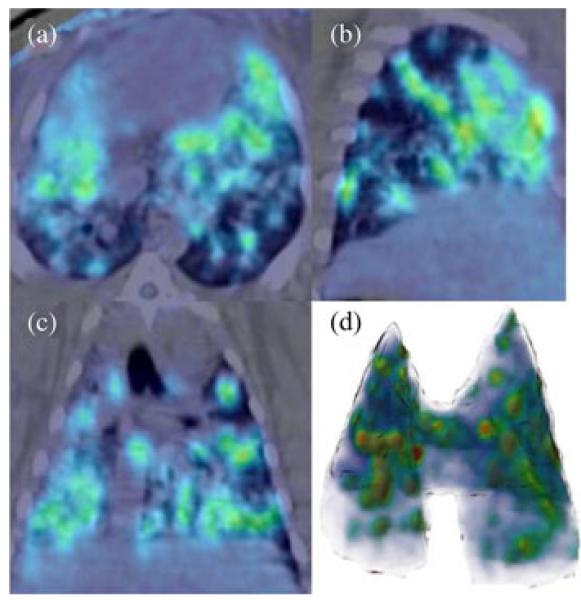
Unlike the focal uptake observed in tumor masses, inflammation in the setting of infection can be spatially diffuse with illdefined borders near or adjacent to normal surrounding anatomical structures [3]. Spatially diffuse or multi-focal abnormal radiotracer uptake with vague margins can limit the precise measurement of disease severity, lesion volume, and metabolic activity of the infected lesions. Fig. 1, for instance, shows typical diffuse and multi-focal radiotracer uptake on an example axial (a), sagittal (b), and coronal (c) slice of a PET image from a rabbit lung infected with tuberculosis (TB). In Fig. 1(d), the volume rendition of the diffuse uptake regions is also demonstrated for three-dimensional (3-D) visualization.

Fig. 1.

(Color online.) Example of a TB infected rabbit lung that shows diffuse and multi-focal areas of radiotracer uptake. (a) axial, (b) sagittal, and (c) coronal slice of the rabbit are shown, and a lung volume rendering is provided in (d).

Quantification studies of pulmonary infection have focused mostly on monitoring the disease using qualitative or semiquantitative image analysis techniques [4]. Given this limitation, the maximum standardized uptake value (SUV_max) is the most commonly used semiquantitative imaging marker derived from PET images, and it has been shown that SUV_max may identify whether a suspicious lesion is malignant or benign [5]. Although this marker is currently the state of the art in routine clinics for various cancer types, in pulmonary infection there is no clear consensus on the use of SUV_max. For instance, a recent pilot study reported that the number of PET active lesions (i.e., TB lesions) rather than SUV_max was predictive of successful TB treatments [6]. Another study [7] demonstrated that the dynamic relationship between pathogen and host responses adds an additional layer of complexity in assessing the imaging parameters with outcomes (i.e., improvement versus disease progression); therefore, one needs to assess nearby structures of the regions with high uptake in order to accurately detect those regions.

Besides the conventional SUV_max measurements of lesions, the number of lesions, their volumes, total lesion activity per lesion, their spatial positions, and interaction with nearby structures should be included in the quantification process for completeness. All of these measurements are prone to errors and are extremely tedious when done manually because of the unique challenges brought by the spatially diffuse multifocal characteristics of metabolic radiotracer activity within the lung. Due to all these hurdles, accurately detecting and efficiently determining lesions’ morphology is necessary to determine the disease state and its progression [8]. In other words, an accurate image segmentation is required 1) to measure metabolic activity of lesions after precisely detecting them; 2) to track disease progression over time using the metabolic tumor volume (MTV), SUV_max and the amount of lesion information (i.e., total lesion activity); and 3) to determine spatial extent of lesions pertaining to pulmonary infections. For accurate quantification of pulmonary infections, most segmentation techniques for PET images are not satisfactory when accomplishing these three necessary conditions because they seemingly ignore the spatial interaction of uptake regions with their nearby tissues.

Since the literature on PET image segmentation is vast, we refer to a recent survey paper for a broad review on this subject [9]. Herein, we will only focus on the state-of-the-art segmentation methods within the scope of our problem description. Although good contrast and poor resolution of PET images motivate the use of thresholding-based approaches for delineating the lesions, there is no clear consensus on how to select an optimal threshold value [9]-[11]. For optimal thresholding, many thresholding techniques from phantom-based analytic expressions were proposed by considering the local geometry of the uptake regions [12]-[14]. However, these techniques are only optimized for focal uptake regions due to the research focus on quantifying cancerous lesions on PET images and are suboptimal for diffuse uptake regions, which often occur in pulmonary infections such as TB (see Fig. 1). Thresholding, followed by some manual correction (arguably, it can be named manual segmentation too), is another common technique used in the clinical setting. The manual correction is necessary due to the suboptimality of the manually chosen threshold. Additionally, manual correction is not only time consuming, but it also has the significant drawback of high inter- and intra-observer variation, along with other disadvantages [15].

More advanced techniques such as fuzzy locally adaptive Bayesian [16], graph-cut [17], random walk [18], [19], and clustering-based methods such as fuzzy c-means [20], k-means [21], etc., were proposed as alternatives to thresholding-based segmentation methods. Thus far, most of these methods are not generally suitable for quantifying infectious diseases because they focus on delineating focal uptake and are suboptimal for spatially diffuse uptake delineation. Also, they can be computational expensive, relatively sensitive to user inputs [22], and fail to converge for spiculated cases [17], [18], [22], [23].

In this study, we present a novel segmentation algorithm based on a segmentation by clustering approach for which the affinity propagation (AP) clustering algorithm is used to find optimal threshold levels for clustering uptake regions. The proposed method leads to a more accurate target definition without the need for incorporating prior anatomical knowledge, and it demonstrates higher accuracy and efficiency compared to current state-of-the-art methods. Our algorithm is naturally tuned for spatially diffuse uptake regions; therefore, it is very useful for quantifying infectious lung diseases.

II. Methods

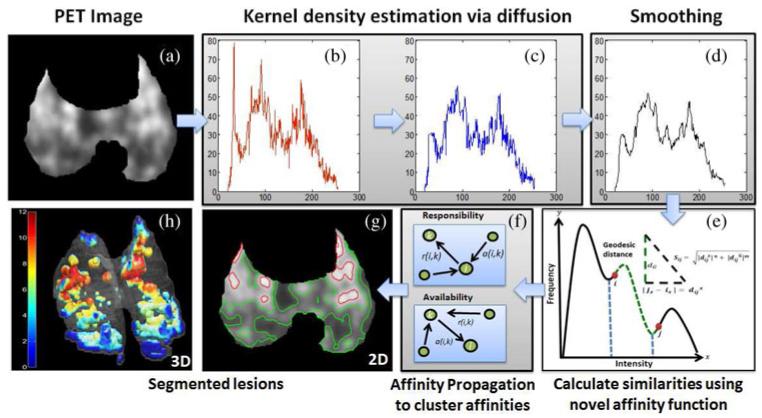
Since PET images are low resolution (relative to CT and MRI) and have high contrast, automated thresholding-based segmentation methods are preferable. This is because intensity histograms of PET images can provide sufficient information for separating objects from the background [24]. Although there are many methods in the literature proposing an automatic threshold selection for PET image segmentation, none of those can provide an optimal thresholding technique for analysis of diffuse uptake in PET images due to large variability of pathology, high uncertainties in object boundaries, low resolution, and the inherent noise of PET images. Therefore, the selection of optimal threshold level(s) has remained a challenging goal. In this study, we address this challenge by introducing a novel affinity function for AP-based clustering to reflect the diffuse and multifocal nature of the uptake regions. Fig. 2 shows the pipeline for the proposed method in quantifying lesions pertaining to TB. After lung regions are delineated from CT images using region growing, PET images are masked with those lung regions to constrain our analysis to infected regions only (a). Then, the kernel density estimation (KDE) via diffusion algorithm is conducted to construct the histogram of the PET images (b), which are next smoothed in (c) and (d). Based on the novel affinity function calculated over the smoothed histogram (e), AP algorithm (f) is used to cluster the PET image voxels into local groups (g). Once delineation of the multi-focal and diffuse uptake regions is completed, quantitative and qualitative metrics are used to evaluate and visualize functional volume of the pathology within the lung regions (h). Details of each step of the proposed framework are described in the following sections.

Fig. 2.

(Color online.) Here is an overview of the proposed PET segmentation framework. For (a) a given PET image and (b) its histogram, (c) its pdf is estimated by KDE via diffusion. (d) The smoothed pdf is used to derive novel similarity parameters (e) which are then clustered using affinity propagation (f). Resulting segmentations are shown in (g) 2-D and (h) 3-D. The colorbar in (h) shows the SUV_max level of the lesions.

A. Kernel Density Estimation Via Diffusion

Traditionally, the histogram had been used to provide a visual clue for the general shape of the probability density function (pdf) [25]. For example, in multivariate density estimation, the following assumption has been used extensively throughout the literature: the observed histogram of any image is the summation of histograms from multiple underlying objects “hidden” in the observed histogram. Objects in the example histogram, shown in Fig. 3, can be approximated by the location of the valleys between peaks, with some inherit uncertainty in the areas of overlap [24]. Based on this, our proposed method assumes that a peak in the histogram corresponds to a relatively more homogeneous region in the image; it is very likely that a peak involves only one class. The justification behind this assumption is that the histogram of objects, in medical images, are typically thought of as the summation of Gaussian curves, which implies a peak corresponds to a homogeneous region in the image(s).

Fig. 3.

(Color online.) Proposed calculation for the affinity between points i and j on the histogram. Objects O₁, O₂, and O₃ represent the classifications that can be made from the gray level histogram.

Due to the nature of medical images, histograms tend to be very noisy with large variability. This makes the optimal threshold selection for separating objects of interest burdensome. First, the histogram of the image needs to be estimated in a robust fashion such that an estimated histogram is less sensitive to local peculiarities in the image data. Second, the estimated histogram should be more sensitive to the clustering of sample values such that data clumping in certain regions and data sparseness in others–particularly the tails of the histogram–should be locally smoothed. To avoid all these problems and provide reliable signatures about objects within the images, herein we propose a framework for smoothing the histogram of PET images through diffusion-based KDE [26]. KDE via diffusion deals well with boundary bias and is much more robust for small sample sizes, as compared to traditional KDE. We detail the steps of the KDE as follows.

1) Traditional KDE uses the Gaussian kernel density estimator [26], but it lacks local adaptation; therefore, it is sensitive to outliers. To improve local adaptation, an adaptive KDE was created in [26] based on the smoothing properties of linear diffusion processes. The kernel was viewed as the transition density of a diffusion process, hence named as KDE via diffusion. For KDE, given N independent realizations, X_{u∈{1,…,N}}, the Gaussian kernel density estimator is conventionally defined as

$$g(x;t)=\frac{1}{N}\sum _{u=1}^N\varphi (x,X_u;t),x\in \mathbf{R}$$ (1)

where

$$\varphi (x,X_u;t)=\frac{1}{\sqrt{2\pi t}}{e}^{-{(x-X_u)}^2∕\left(2t\right)}$$

is a Gaussian pdf at scale t, usually referred to as the bandwidth. An improved kernel via diffusion process was constructed by solving the following diffusion equation with the Neumann boundary condition [26]:

$$g^{\mathrm{diff}}(x,X_u;t)=\sum _{z=-\infty }^{\infty }\left(\varphi \right(x,2z+X_u;t)+\varphi (x,2z-X_u;t\left)\right)x\in [0,1].$$ (2)

2) After KDE via diffusion, an exponential smoothing was applied to further reduce the noise; the essential shape of the histogram was preserved throughout this process (see Fig. 4 for an example smooth KDE conducted on the PET image histogram). Data clumping and sparseness in the original histogram (left) were removed (middle), and any noise remaining after KDE via diffusion was reduced (right) considerably while still preserving the shape of the pdf. The resultant histogram can now serve as a proficient platform for the segmentation of the objects, as long as an effective clustering approach can locate the valleys in the histogram.

Fig. 4.

(Left) Original histogram from PET image of a masked rabbit lung. (Middle) Histogram after KDE via diffusion and piecewise cubic interpolation. (Right) Final histogram after exponential smoothing with window size = 20. The approximate shape of the original histogram is preserved.

B. Affinity Propagation

Affinity propagation was first proposed by Frey and Dueck [27] for partitioning datasets into clusters, based on the similarities between data points. AP is useful because it is efficient, insensitive to initialization, and produces clusters at a low error rate. Basically, AP partitions the data based on the maximization of the sum of similarities between data points such that each partition is associated with its exemplar (namely its most prototypical data point) [28]. Unlike other exemplarbased clustering methods such as k-centers clustering [21] and k-means [29], performance of AP does not rely on a “good” initial cluster/group. Instead, AP obtains accurate solutions by approximating the NP-hard problems in a much more efficient and accurate way [27], [28]. AP can use arbitrarily complex affinity functions since it does not need to search or integrate over a parameter space. Due to the flexibility of the AP method regarding the affinity function definition, we explored a novel affinity function that best suited PET image segmentation effectively, where the radiotracer uptake regions were distributed widespread over the lungs.

1) Background on AP

AP initially assumes all data points (i.e., voxels) as exemplars and refines them down iteratively by passing two “messages” between all points: responsibility and availability. Messages are scalar values such that each point sends a message to all other points, indicating to what degree each of the other points is suitable to be its exemplar. The first message is called responsibility, indicated by r(i, k), and is how responsible point k is to be the exemplar of point i. In availability, denoted by a(i, k), each point sends a message to all other points and indicates to what degree the point itself is available for serving as an exemplar. These messages are sent iteratively until the messages do not change. The responsibility and availability were formulated in Frey and Dueck’s original paper as

$$r(i,k)\leftarrow s(i,k)-\underset{k^{\prime }\{k^{\prime }\ne k\}}{\max }\left\{a\right(i,k^{\prime })+s(i,k^{\prime }\left)\right\}$$ (3)

$$a(i,k)\leftarrow \min \left\{0,r(k,k)+\sum _{i^{\prime }\{i^{\prime }\notin i,k\}}\max \{0,r(i^{\prime },k\left)\right\}\right\}$$ (4)

where s(i, k) is the similarity between point i and point k, and k′ is all other points except for i and k. Point k is not responsible to be the exemplar for point i if there is another point that describes i better than k; hence, the maximum value for responsibility is reached. The sum of availabilities and responsibilities at any iteration provides the current exemplars and classifications. Initially, all points are considered to be possible exemplars, which guarantees globally optimal solutions [27].

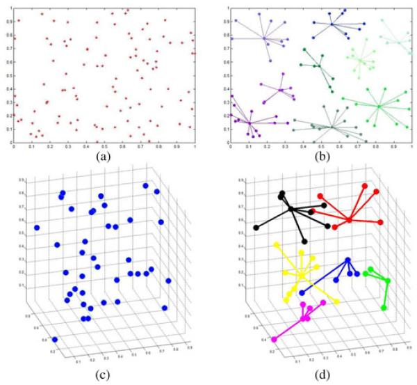
AP uses max-product belief propagation to obtain good exemplars through maximizing the objective function argmax_k[a(i, k) + r(i, k)]. When k = i, the responsibility, r(k, k), is set to the preference. The preference of a data point is set between 0 and 1, where 0 always prevents this point from being an exemplar and 1 always makes this point an exemplar. If the preference is anywhere between 0 and 1, AP will not necessarily make that point an exemplar, but AP will use this prior information to cluster the data. Fig. 5 illustrates examples of AP applied to both 2-D (a) and 3-D (b) randomly generated points and their resulting groups (c) and (d), shown in various colors. The exemplar is the center point of each group and all other points in the group are connected by it. The preference of all the data was arbitrarily set between 0 and 1. It made no difference on the clustering result because all points were equally likely to be exemplars initially. In our implementation, we also allowed the AP to be semi-supervised by allowing the user to change the preference of a data point (see Section III-H for details).

Fig. 5.

(Color online.) (a) and (b) Examples of exemplar-based AP clustering results on 100 2-D randomly generated points. (c) and (d) are AP applied to 40 randomly generated 3-D points and their groupings. For both examples, the center point of each group is the groups exemplar.

2) Novel Affinity Metric Construction

We developed a novel affinity metric to model the relationship between all data points using the accurately estimated histogram with the main assumption that closer intensity values are more likely to belong to the same tissue class. In other words, the data is composed of points lying on several distinct linear spaces, but this information is hidden in the image histogram, given that the histogram is carefully estimated in the previous step. This segmentation process recovers these subspaces and assigns data points to their respective subspaces. In the process, similarities among the voxels play a vital role. Most clustering methods are focused on using either Euclidean or Gaussian distance functions to determine the similarity between data points. Such a distance is straightforward in implementation; however, it drops the shape information of the candidate distribution [30]. To incorporate this fact into an improved definition of an affinity function, we propose a new affinity model where similarity between any two points are described in the non-Euclidean space through the geodesic distance definition by taking both intensity- and probability-based measures into account.

Fig. 3 demonstrates the proposed affinity metric calculation on the estimated histogram (normalized to obtain the pdf): the larger the probability difference between points i and j is (i.e., |p_i - p_j|), the smaller the probability for having the same label for data points i and j. In contrast to this probability-based constraint, a simple intensity difference from data points i and j denotes the edge (or gradient) information. The large intensity difference between i and j implies a high possibility of two (or multiple) objects within the range of i and j; therefore, a threshold between i and j can separate the objects.

Because both probability- and intensity-based differences of any two voxels carry valuable information on the selection of appropriate threshold determination, we propose to combine these two constraints within a new affinity model. These constraints can simply be combined with weight parameters n and m as follows:

$$s(i,j)=-{({\mid d_{ij}^x\mid }^n+{\mid d_{ij}^G\mid }^m)}^{1∕2}$$ (5)

where s is the similarity function, $d_{ij}^G$ is the computed geodesic distance between point i and j along the pdf of the histogram, and $d_{ij}^x$ is the Euclidean distance between point i and j along the x-axis.

Note that the geodesic distance between the two data points in the image naturally reflects the similarity due to the gradient information (i.e., voxel intensity differences). It also incorporates additional probabilistic information via enforcing local groupings for particular regions to have the same label. We computed the geodesic distance, d^G, between data points i and j as the sum of local Euclidean distances using all points between i and j, without the need for any polynomial interpolation between the points (which may introduce additional errors) as

$$d_{ij}^G=\sum _{k=i}^{j-1}{d}_E(k,k+1),\text{where}j>i.$$ (6)

Once the similarity function is computed for all points, AP tries to maximize the energy function $E\left(\mathrm{c}\right)={\Sigma }_{i=1}^{N}s(i,c_i)+{\Sigma }_{k=1}^N{\delta }_k\left(\mathrm{c}\right)$ where assignment vector c can be derived from argmax_k[a(i, k) + r(i, k)]. Note that c includes N hidden labels corresponding to N data points, and each c_i indicates the exemplar to which the point belongs (i.e., c_i = j if point j is an exemplar of the point i). Furthermore, an exemplar-consistency constraint δ_k(c) can be defined as [27]

$${\delta }_k\left(\mathrm{c}\right)=\{\begin{array}{cc}-\infty \hfill & \text{if}{c}_k\ne k\text{but}\exists i:c_i=k\hfill \\ 0,\hfill & \text{otherwise}.\hfill \end{array}\phantom{\}}$$ (7)

This constraint enforces valid configuration by introducing a large penalty if some data point i has chosen k as its exemplar without k having been correctly labeled as an exemplar. After inserting a novel affinity function definition into the energy constraint to be maximized within the AP algorithm, we obtained the following objective function:

$$E\left(\mathrm{c}\right)=-\sum _{i=1}^N{({\mid d_{i{c}_i}^x\mid }^n+{\mid d_{i{c}_i}^G\mid }^n)}^{1∕2}+\sum _{k=1}^N{\delta }_k\left(\underset{k}{\mathrm{argmax}}\right[a(i,k)+r(i,k)\left]\right).$$ (8)

Finally, all voxels are labeled based on the optimization of the objective function defined above. Since the update rules for AP correspond to fixed-point recursions for minimizing a Bethe free-energy approximation [27], AP is easily derived as an instance of the max-sum algorithm in a factor graph [31] describing the constraints on the labels and the energy function.

III. Experiments and Results

Our proposed method was tested using PET rabbit lung images with varying levels of diffuse uptake. Since rabbits were scanned in PET and CT scanners separately, we needed to register PET images into their CT counterpart. We used a locally affine and globally smooth registration framework to register all images [32], [33]. Manual adjustment was conducted by two expert observers when necessary. Region growing-based lung segmentation from CT scans was done to create lung masks, and then each lung mask was used to filter out the lung portion from the corresponding PET images as a preprocessing step. Other lung segmentation algorithms can also be used for this purpose [34]. PET image segmentation results were compared to manual delineations, i.e., surrogate truths, provided by the expert observers, as well as the state-of-the-art PET segmentation methods. All experiments were conducted using the unsupervised (fully automated) version of the proposed method for an unbiased evaluation for its performance.

A. Tuberculosis in Small Animal Models

Ranging from preinfection to 38 weeks postinfection (0, 5, 10, 15, 20, 30, and 38 weeks), 70 PET scans from 10 rabbits were evaluated. The rabbits were aerosol infected with Mycobacterium TB (H37Rv strain) in a Madison chamber, implanting 3 × 10³ bacilli into the lungs. The rabbits were injected via the marginal ear vein, with 1-2 mCi of 18F-FDG PET and imaged 45-min postinjection with 30 min static PET acquisition. All CT and PET imaging was performed without respiratory gating on the NeuroLogica CereTom and the Philips Mosaic HP scanner, respectively.

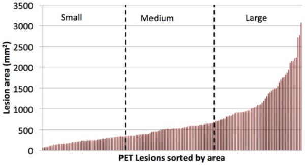
Evaluation of the segmentation was conducted on a subset of randomly selected slices among different rabbits and time points since manual segmentation of the diffuse uptake regions of all the images was too laborious and time consuming. The random selection was done in order to minimize any slice selection bias and introduce a representative segmentation evaluation framework. A total of 168 slices were selected to be used in the TB metabolic volume quantification. In this process, two experts manually segmented the significant uptake regions using 2-D manual thresholding, namely the current clinical standard for spatially diffuse uptake. Necessary manual correction was also conducted. In order to further assess our method’s performance on various lesion sizes, the lesions were split into three groups (i.e., small, medium, and large) according to their areas. These cutoffs were carefully selected to ensure that the same number of lesions was in each group, and the cutoffs were similar to the ones found in the literature [35]. The main premise behind this approach was to show that our method was not overestimating smaller lesions, as opposed to the state-of-the-art methods, and not underestimating large uptake regions due to the diffuse nature of the uptake. The groups were defined as small (0 – 3.45 cm²), medium (3.45 – 6.84 cm²), and large (6.84 – 30.67 cm²), with 56 lesions per group. Fig. 6 summarizes the distribution of lesion areas and the group cutoffs selected.

Fig. 6.

TB lesions were sorted by area found from expert segmentation and divided into 3 groups small (0–3.45 cm²), medium (3.45–6.84 cm²), and large (6.84–30.67 cm²) with equivalent number of lesions per group. A large variation of sizes was used to remove bias from the segmentation results.

B. Quantitative and Qualitative Evaluation

The Dice Similarity Coefficient (DSC)–a coefficient that measures the overlap between two segmentation results–and the “sensitivity (TPVF),” and “specificity (100-FPVF)” (i.e., TPVF: true positive volume fraction, FPVF: false positive volume fraction) were calculated between the segmented region that was found by the proposed method and the expert delineations. Table I lists all evaluation results with above mentioned measures. The average DSC was found to be 91.25 ± 8.01% for all lesions when comparing the proposed method to the segmentation result using the average of the two expert defined delineations. A sensitivity of 88.80 ± 12.59% and a specificity of 96.01 ± 9.20% were achieved. Overall, the DSC, sensitivity, and specificity rates increased with larger lesion area, as expected.

TABLE 1. Segmentation Evaluations of PET Images.

Experiment	DSC(%)	TPVF(%)	(1-FPVF)(%)	DSC(%)	TPVF(%)	(1-FPVF)(%)
	Small Lesions (0–3.45cm2)			Medium Lesions (3.45 – 6.84cm2)
Observer 1 to Proposed Method	89.38±9.24	90.14±14.02	89.64±14.20	89.20±10.06	95.63±8.88	86.20±16.30
Observer 2 to Proposed Method	87.23±9.35	85.17±15.86	95.82±8.40	88.72±9.50	83.59±15.63	97.26±5.92
Average* to Proposed Method	91.25±8.66	86.85±14.90	96.22±8.06	91.46±8.60	92.05±11.11	93.23±12.58
Observer 1 to Observer 2	84.91±8.20	93.98±12.12	87.87±12.78	86.14±10.26	98.46±4.88	78.50±16.23
	Large Lesions (Greater than 6.84cm2)			Total Lesions
Observer 1 to Proposed Method	90.80±6.35	93.69±8.59	89.99±12.26	89.38± 8.71	92.93±11.06	88.89±14.32
Observer 2 to Proposed Method	85.67±10.28	77.79±15.38	98.41±6.46	87.21±9.93	81.02±15.83	97.54±6.85
Average* to Proposed Method	91.80± 7.17	88.07±11.66	97.49±6.78	91.25± 8.01	88.80±12.59	96.01±9.20
Observer 1 to Observer 2	81.90± 13.11	99.40±2.55	71.90±18.70	84.91±11.65	97.76±7.17	77.65±17.85

^*Average refers to the segmentation resulting from the average thresholding value between the two expert observers.

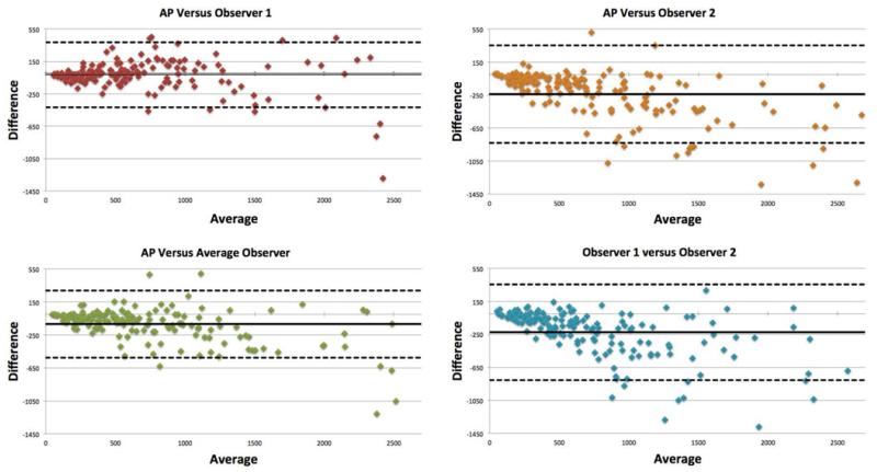
Fig. 7 shows four linear regression graphs for segmentation evaluation of the proposed method with respect to the observers. An inter-observer agreement between observers was also reported in the same figure. The correlation between the proposed method versus the average between the observers was reported as R² = 0.906, (p < 0.01). Similarly, Bland–Altman plots were constructed in Fig. 8 to show an excellent agreement between the proposed method and expert delineations, where outliers are the points outside the 95% confidence interval (i.e., dotted lines).

Fig. 7.

Linear regression graph of the segmentation area from our proposed method versus observer 1, observer 2, and the average threshold segmentation between observer 1 and 2. The segmentations provided by observer 1 and observer 2 are plotted to demonstrate the large inter-observer variation.

Fig. 8.

Bland–Altman plot of results from the PET rabbit lung images. The solid line represents the mean difference between the two segmentations while the dashed lines is the 95% confidence interval.

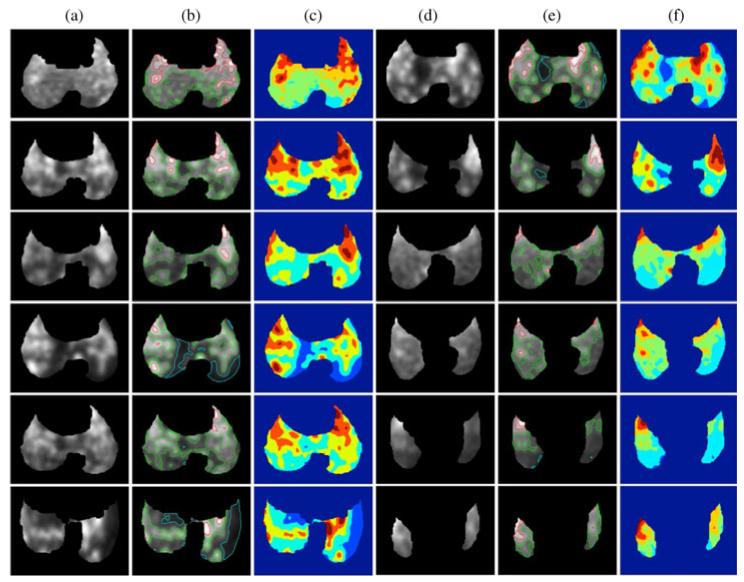
For a qualitative comparison, the segmentation results from 12 example PET slices, all from infected rabbit lungs, are shown in Fig. 9. Columns A and D show the original PET image of the lung, while columns B and E show the boundary information of the various groups on the original PET image. Columns C and F color each group for a better visualization, and it can be readily seen that each group is homogeneous to some extent.

Fig. 9.

(Color online.) Segmentation results of PET images from the rabbit model. (a) and (d) Original PET images. (b) and (e) original image is overlaid with the segmentation boundaries found from the proposed method. (c) and (f) the same segmentation result is also provided in a different visualization with colored group labels.

C. Comparison With the State-of-the-Art Methods

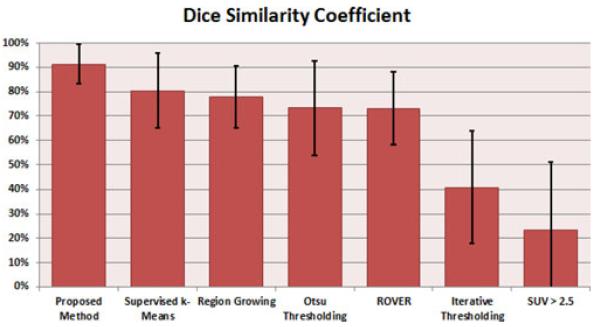
We compared our approach with the commonly used PET image segmentation techniques: RG [36], k-means, various adaptive thresholding-based methods, as well as the Region of interest Visualization, Evaluation, and image Registration (ROVER) software (ABX GmbH, Radeberg, Germany). Fig. 10 shows the accuracy comparison of segmentation results with these state-of-the-art methods. Our proposed method had the highest DSC, sensitivity, and specificity, while supervised k-means performed the second best.

Fig. 10.

Quantitative results of proposed method versus several sate-of-the-art methods against the average expert thresholding value. Supervised k-Means is k-Means using manually defined number of clusters per image.

For the thresholding-based methods, we first compared them to the current clinical standard for thresholding malignant tumors on PET images as SUV_max > 2.5 [5], which performed poorly for the small animal TB model. Two other thresholding methods were also compared to the proposed method: Otsu Thresholding [11], 73.27 ± 19.42%, and the Iterative Thresholding Method (ITM) [10], 40.76 ± 23.01%. While the Otsu thresholding method performed similar to the RG method, ITM and SUV-based fixed thresholding methods did not perform well due to the diffuse and multifocal uptake nature of the uptake regions. Our proposed method consistently resulted in higher DSC values than the thresholding-based methods.

ROVER uses an adaptive thresholding and background subtraction algorithm to identify lesion volume within a mask and is already in clinical use in Europe [37]. It performed very similar to the Otsu thresholding method with a DSC of 73.14 ± 14.86%. This software is designed for 3-D ROI analysis and volume determination. We found that in many cases the ROVER automatic segmentation agreed with the proposed method, but in some cases it included the areas of the PET images that the expert delineations had previously determined as nonsignificant uptake. For diffuse uptake, it is a very difficult task to include only the significant uptake and to disregard the other areas which is needed for proper quantification of the disease severity in small animal models. We conclude that ROVER may not be suited for the segmentation of small animal TB models as the supervised k-means outperformed it.

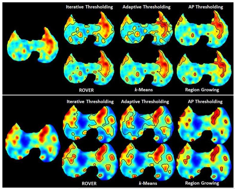
Finally, k-means, a commonly used clustering method [38], [39], was also compared to the proposed method. A major drawback of k-means and most clustering methods is that they require the user to specify the number of groups to cluster, which is traditionally two, i.e., a foreground and background. However, given the diffuse and multifocal nature of the TB images, an expert manually specified the number of groups based on the appearance of the images instead of just using the traditional two groups, and found a DSC of 80.40 ± 15.31% (see Fig. 10). Nevertheless, the overall performance of supervised k-means was inferior to our proposed method. Fig. 11 gives a qualitative comparison of the state-of-the-art PET image segmentation methods that were compared to, excluding the SUV > 2.5 thresholding.

Fig. 11.

(Color online.) Qualitative comparison of several state-of-the-art PET image segmentation methods. For the proposed method, AP Thresholding, only the boundary of the highest uptake group is shown for easier comparison.

D. Robustness Analysis of the Proposed Method and Evaluation by Phantoms

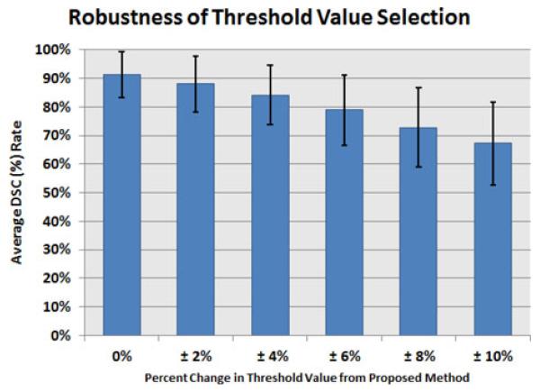
In order to further assess how robust the determined thresholding levels were, we conducted additional experiments by altering the thresholding values using the proposed method through a percent change (±0, 2, 4, 6, 8, 10%) and exploring how DSC rates were being affected with respect to the given reference truths. Based on each altered threshold level, we resegmented the PET images and recalculated the DSC values. Results are summarized in Fig. 12. As can be depicted from the results, a small change in the thresholding level (around ±2%) decreased the DSC values; however, these changes can be regarded as non-significant. More than ±2% changes in the threholding levels can cause further decrease in the segmentation results due to high variation in the diffuse uptake regions. Together with the results obtained from robustness experiments, and considering the high inter-observer variation when determining near-optimal thresholding, it can be concluded that the automatically determined threshold levels found through the proposed method gives the best possible threshold levels for grouping diffuse uptake regions.

Fig. 12.

Analysis of the robustness of the threshold value selection was performed. The images were segemented using percent changes of the thresholding values found using the proposed method and DSC value is calculated.

When evaluating segmentation algorithms, it is often desired to have ground truths instead of surrogate truths. In PET imaging, various phantoms were designed for this purpose; however, most of such phantoms are not realistic due to inaccurate noise assumptions and limited spatial resolutions of the PET scans. Another shortcoming is that digital phantoms include spherical lesions (due to cylindirical set up in CT base) and they do not reflect the underlying uptake pattern commonly seen in pulmonary infections (multifocal and diffuse). Nevertheless, we evaluated the efficacy of our proposed algorithm by using IEC image quality phantoms (NEMA standard) [40] to demonstrate its feasibility when the ground truth is known. The IEC phantoms contained six spherical lesions of size 10, 13, 17, 22, 28, 37 mm in diameter with two different signal to background ratios (SBRs) (i.e., 4:1 and 8:1) and the voxel size were 2 mm × 2 mm × 2 mm. Resulting PET segmentations by the proposed algorithm were compared with the ground truth, which was simulated from CT, and the following dice scores were obtained: 90.6 ± 2.9% for SBR = 4:1, and 96.1 ± 3.2% for SBR = 8:1. Further details of the phantoms and their appearance can be found in [23] and [40]. As pointed out earlier, we believe that the use of the phantoms with spherical uptake realizations (i.e., focal uptake) is suboptimal for evaluating our proposed method’s success in non-spherical uptake realizations. This limitation is revisited in the discussion section.

E. Effect of Different Parameterization on the Novel Affinity Function

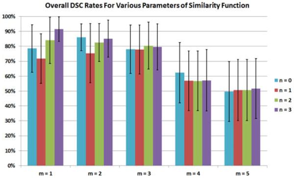
The proposed affinity function has two weighting parameters n and m (see equation 5). We set these parameters based on histograms of the PET images used in a training step (training images were not used in testing). Segmentation evaluations presented in the quantitative and qualitative evaluation section were based on the optimal parameters we found in this step. In order to demonstrate how the novel affinity function behaved for different n and m values, we conducted additional experiments using various parameter pairs. For simplicity, m was selected to be an integer between 1 and 4 to reflect the contribution of geodesic distance-based similarities, while n was ranged from 0 to 3. Results without contribution of the geodesic distance-based similarity metric (i.e., when m = 0) are discussed in the next section.

Different combinations of these constraints are possible; however, due to the fast convergence of power series and the intuitive meaning of the local Euclidean distances, we prefer to retain the combined affinity formulation in linear form. Note that with the current implementation of the affinities, the similarity function is still symmetric and elements of the similarity matrix are kept smooth with appropriately chosen weight parameters n and m. For different combinations of these parameters, PET images were resegmented and the resultant DSC rates are given in Fig. 13. We observed the best performance when n = 3 and m = 1; however, it would be different for other imaging datasets such as human patients. For m > 2, the variability between different n values was small, most likely because the geodesic term in the novel affinity function was much greater and had a stronger effect on the affinity value than the gradient term for these parameterizations.

Fig. 13.

(Color online.) Testing images were segmented using various parameterization for n and m in the proposed affinity function. The DSC results as compared to the expert defined ground truth are provided.

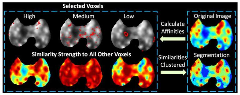
Fig. 14 gives a qualitative view on the strength of affinities in an example PET image using the proposed affinity function with the original image shown in the top right. After the histogram was estimated using the framework described previously, three example intensity levels were selected (named high, medium, and low) and the voxels with these intensities (specified by red dots overlaid onto the original image) are shown in the top row of Fig. 14. For each of the three example intensity levels, the affinity to all other voxels on the image was calculated. The strength of the affinities, shown in the bottom row, gives an intuition on how the affinity function behaves in a qualitatively manner (i.e., red represents a stronger affinity strength, while blue represents a weaker strength). Finally, the affinities between all the intensities, not just the three example intensities, were calculated and then clustered using AP. The resulting segmentation is given on the bottom right.

Fig. 14.

(Color online.) The strength of the affinities using the proposed affinity function applied to three selected example intensities (specified by red dots on the original image in the top row) is given using red to signify a stronger affinity while blue represents a weaker strength (bottom row). The final segmentation is given in the bottom right.

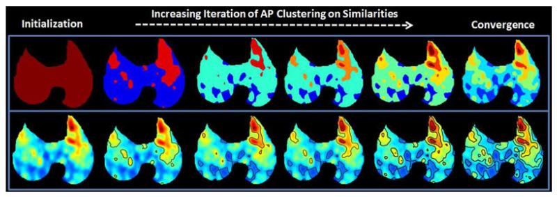
At any iteration of the AP clustering, the current exemplars and clusters can be determined and can shed light on how the algorithm moves toward convergence. For this, we examined the segmentation result at several iterations and the results are demonstrated in Fig. 15. The top row shows the current segmentation in color coded groups, while the bottom row gives the segmentation boundary on the original PET image. Each column of Fig. 15 is a different iteration (in increasing order) of the AP clustering using the proposed affinity calculation. The last column shows the final segmentation result obtained when iterations are converged to a steady state.

Fig. 15.

(Color online.) AP clustering algorithm allows the identification of the exemplars at any iteration. A qualitative view on the convergence of the proposed method is provided.

F. Evaluation of Other Affinity Functions

We also investigated different ways of computing the affinity functions within the AP clustering that may serve as potential similarity metrics for delineating multifocal and diffuse uptake regions. For example, by taking into account only the geodesic distance between the data along the histogram, a Gaussian distance function can be used to define the affinity between the points as

$$s(i,j)=-\exp \left(-\frac{d_{ij}^G}{{\sigma }^2}\right)$$ (9)

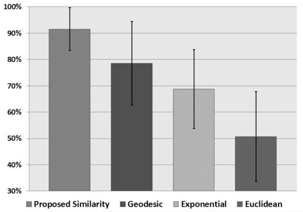
where σ is a constant showing variation. Here, we called this affinity construction the exponential distance function. The main advantage of this affinity calculation is the ability to vary σ along the curve to influence the size of the object found. Potentially, this method could correctly group a histogram with a very large variation in the group size. However, as noted earlier, the major drawback was how to adapt the σ value within a histogram to account for the local variations in group sizing. The approximate location of these peaks must be known beforehand and due to the significant variation and noisy nature of PET image histograms, (9) may not be a very robust metric. Therefore, to give an approximate performance of this Gaussian distance function as an affinity function, we chose a constant σ for all the images and tested the segmentation accuracy. In addition, we also evaluated the performance using the Euclidean distance between the data points as the affinity function as well as using only the geodesic distance. The results of these experiments are provided in Fig. 16. For the four definitions of the affinities, the proposed metric outperformed the others with an average DSC value of 91.25 ± 8.01%. Notably, utilizing the Euclidean distance as the affinity function segmented with an accuracy of 50.76 ± 16.96%, whereas the sole use of Geodesic distance resulted in segmentation accuracy of 78.57 ± 15.89%. Compared to Euclidean and Geodesic distance, the exponential distance had an accuracy of 68.77 ± 15.02%. Our experiments validated that the use of the proposed affinity function was well suited for diffuse and multifocal uptake regions in PET images compared to other possible affinity functions commonly used in the literature for different applications.

Fig. 16.

DSC rates between the proposed segmentation framework utilizing different affinity functions as compared to the ground truth. Geodesic is utilizing only the geodesic distance as a similiarity function between the data point. Euclidean refers to the Euclidean distance while exponential refers to the Gaussian distance function.

G. Computational Cost and Parameter Settings

The parameters for AP were set as follows: in the AP algorithm, each message is set to λ times its value from the previous iteration plus 1 – λ times its prescribed updated value, where the damping factor λ is between 0 and 1. In the original AP formulation [27], the damping factor was set to 0.5; however, in our PET image segmentation experiments, it was sufficient in all cases when the damping factor was set to λ = 0.8. For the convergence of the AP clustering, the maximum number of iteration was set to t_max = 500, and the average iteration number for the convergence was found to be less than 100 in all cases. The threshold level for the diffusion-based KDE method was 10%, while a window size of 20 was used for the exponential smoothing. The proposed method can be run either in 2-D or 3-D. It took 0.66 seconds per slice (2-D computation) and around 1 min for 3-D computation on an Intel workstation with 24-GB memory running at 3.10 GHz. The computation times of the state-of-the-art methods that we compared to our proposed method were similar. After the proposed method, the fastest methods were the Otsu thresholding and Iterative thresholding which on average took 1.3 s and 1.5 s per slice, respectively. The k-means took 4.5 s, while the ROVER software took 7.5 s per slice. Finally, the region growing took about 12 s per slice due to the need for manual seed selection on all the multifocal uptake on the testing images.

H. Semi-supervised Affinity Propagation

Our proposed method can also be used in a semi-supervised manner, allowing a user to select certain image intensities as preferred exemplars. This interaction may be useful because it can force (or influence) the algorithm to form additional local groupings or refine the extent of the local groups to further enhance the delineation result. However, there is a drawback of a slightly longer delineation time, which is mostly consisting of waiting for the user to define the seeds, and the user input adds some inherent variation in the segmentation accuracy. Additional constraints from a user defined seed governs an allowed set of solutions in AP.

For semi-supervised AP, availability and responsibility formulations do not change but the affinity function does. Assume that data point i is similar to j and data point q is similar to t. If j and q must be in the same cluster and a user incorporates this into the proposed framework as an instance constraint, then the similarity between i and t in the original AP formulation alters from s(i, t) < s(i, j) + s(q, t) into $\widehat{s}(i,t)=s(i,j)+s(q,t)$. Finally, the updated affinity $\widehat{s}(i,t)$ is used in responsibility formulation as $r(i,k)\leftarrow \widehat{s}(i,k)-{\max }_{k^{\prime }\{k^{\prime }\ne k\}}\left\{a\right(i,k^{\prime })+\widehat{s}(i,k^{\prime }\left)\right\}$ and in (4) until convergence.

IV. Discussion

Our segmentation evaluation criteria follows the widely accepted segmentation evaluation standards proposed by Udupa et al. [41]. However, one may also consider adding more expert observers into the evaluation framework in order to improve the reliability of the segmentation evaluation framework. For this purpose, simultaneous ground truth estimation tools such as STAPLE [42] can be considered. Nevertheless, as long as the inter- and intra-observer agreements are given with manual labeling, surrogate truths constructed by the limited number of observers are valid and can be used for segmentation evaluation.

This proposed framework for PET image segmentation has a few limitations that should be noted. First of all, if the object of interest has intensities localized in the low frequencies of the histogram (i.e., a much smaller peak as compared to other peaks in the histogram), the framework may not recognize it as a separate object or may assume that it is noise due to the resolution limitation and partial volume effect. Second, objects of interest are assumed to form a peak in the histogram—nearly always the case for objects within PET images—but it is the-oretically possible that an object could consist of exactly the same intensity, with little or no partial volume effect, blurring the edges. If this occurs, the algorithm would most likely treat this as noise because the histogram would be significantly different from the local surrounding points. Finally, the effect of partial volume correction on PET images was kept outside the scope of this paper; nevertheless, there is no obstacle for the proposed method to be used with images that are corrected by a partial volume correction algorithm prior to delineation. Indeed, this additional preprocess has the potential to improve the segmentation accuracy.

It is also important to note that there are some connections between this framework, spectral clustering and Laplacian eigenmaps [43]. Spectral clustering or Laplacian eigenmaps may be adopted within the same framework of ours, but a precise definition of an affinity function will be needed. In addition, the proposed framework and spectral clustering both incorporate the idea of using similarities between data points for clustering, but spectral clustering achieves this classification result by cutting weights between data points. On the contrary, we use AP to cluster the similarities found by the novel affinity function without using any prior assumption on the size or number of points in each group.

Stute et al. [44] simulated highly realistic PET images using Monte Carlo simulations and input activity maps with appropriate spatial resolution and noise level. By doing so, the intrinsic heterogeneity of the activity distribution between and within organs can be accurately modeled. Although Stute’s method is promising for realistic PET simulations and contain spatial resolution and noise parameters from real PET data, sole use of these parameters does not adress the problem of creating multifocal and spatially diffuse uptake patterns. It is because there is also a need for specific geometrical phantom design other than cylindrical-base phantoms in order to mimic underlying patterns of interest. It should also be noted that there is no consensus among clinicians about the exact shape and distribution of the lesions observed in the pulmonary infections apart from its known multifocal and diffuse nature. Hence, the use of commonly available digital phantoms which include spherical lesion realizations may not be optimal for validating the proposed segmentation method. As a potential extension of our study, we consider developing a specific non-speharical geometric-base digital phantom which considers multifocal and diffuse nature of the uptake in PET images followed by a realistic simulations through the Monte Carlo steps as clearly and well defined by Stute et al. [44].

V. Conclusion

Most current PET image segmentation methods are not suitable for distributed inflammation because they focus only on focal uptake; therefore, we proposed a novel segmentation framework to quantify TB disease in functional imaging domain in small animals. We evaluated the robustness and accuracy of the proposed PET segmentation framework against the current state-of-the-art methods and achieved superior results. We conclude that computer-aided quantification of infectious lung disease can be conducted with high accuracy. Our proposed segmentation technique is finely tuned to cluster distributed radiotracer activities within the lung regions, and we showed that our method has the potential to reduce variability when segmenting TB from small animal images.

References

- [1].Bagci U, Bray M, Caban J, Yao J, Mollura DJ. Computer-assisted detection of infectious lung diseases: A review. Comput. Med. Imag. Graph. 2012;36(1):72–84. doi: 10.1016/j.compmedimag.2011.06.002. [DOI] [PMC free article] [PubMed] [Google Scholar]
- [2].Kaufmann P, Camici P. Myocardial blood flow measurement by pet: Technical aspects and clinical applications. J. Nucl. Med. 2005;46(1):75–88. [PubMed] [Google Scholar]
- [3].Zhao B, Schwartz L, Larson S. Imaging surrogates of tumor response to therapy: Anatomic and functional biomarkers. J. Nucl. Med. 2009;50(2):239–249. doi: 10.2967/jnumed.108.056655. [DOI] [PubMed] [Google Scholar]
- [4].Davis S, Nuermberger E, Um P, Vidal C, Jedynak B, Pomper M, Bishai W, Jain S. Noninvasive pulmonary [18f]-2-fluoro-deoxy-d-glucose positron emission tomography correlates with bactericidal activity of tuberculosis drug treatment. Antimicrob. Agents Chemother. 2009;53(11):4879–4884. doi: 10.1128/AAC.00789-09. [DOI] [PMC free article] [PubMed] [Google Scholar]
- [5].Nestle U, Kremp S, Grosu A. Practical integration of [18 F]-FDG-PET and PET-CT in the planning of radiotherapy for non-small cell lung cancer (NSCLC): The technical basis, ICRU-target volumes, problems, perspectives. Radiother. Oncol. 2006;81(2):209–225. doi: 10.1016/j.radonc.2006.09.011. [DOI] [PubMed] [Google Scholar]
- [6].Sathekge M, Maes A, Kgomo M, Stoltz A, de Wiele CV. Use of 18F-FDG PET to predict response to first-line tuberculostatics in HIV-associated tuberculosis. J. Nuclear Med. 2011;52:880–885. doi: 10.2967/jnumed.110.083709. [DOI] [PubMed] [Google Scholar]
- [7].Russell DG, Barry CE, Flynn JL. Tuberculosis: What we don’t know can, and does, hurt us. Science. 2010;328:852–856. doi: 10.1126/science.1184784. [DOI] [PMC free article] [PubMed] [Google Scholar]
- [8].Bagci U, Yao J, Miller-Jaster K, Chen X, Mollura DJ. Predicting future morphological changes of lesions from radiotracer uptake in 18F-FDG-PET images. PlosOne. 2013;8(2):e57105. doi: 10.1371/journal.pone.0057105. [DOI] [PMC free article] [PubMed] [Google Scholar]
- [9].Zaidi H, El Naqa I. Pet-guided delineation of radiation therapy treatment volumes: A survey of image segmentation techniques. Eur. J. Nuclear Med. Molecul. Imag. 2010;37(11):2165–2187. doi: 10.1007/s00259-010-1423-3. [DOI] [PubMed] [Google Scholar]
- [10].Ridler T, Calvard S. Picture thresholding using an iterative selection method. IEEE Trans. Syst., Man Cybern. 1978 Aug;SMC-8(8):630–632. [Google Scholar]
- [11].Otsu N. A threshold selection method from gray-level histograms. Automatica. 1975;11(285-296):23–27. [Google Scholar]
- [12].Erdi Y, Mawlawi O, Larson S, Imbriaco M, Yeung H, Finn R, Humm J. Segmentation of lung lesion volume by adaptive positron emission tomography image thresholding. Cancer. 1997;80(S12):2505–2509. doi: 10.1002/(sici)1097-0142(19971215)80:12+<2505::aid-cncr24>3.3.co;2-b. [DOI] [PubMed] [Google Scholar]
- [13].Black Q, Grills I, Kestin L, Wong C, Wong J, Martinez A, Yan D. Defining a radiotherapy target with positron emission tomography. Int. J. Radiat. Oncol., Biol., Phys. 2004;60(4):1272–1282. doi: 10.1016/j.ijrobp.2004.06.254. [DOI] [PubMed] [Google Scholar]
- [14].Nestle U, Kremp S, Schaefer-Schuler A, Sebastian-Welsch C, Hellwig D, Rübe C, Kirsch C. Comparison of different methods for delineation of 18F-FDG PET-positive tissue for target volume definition in radiotherapy of patients with non–small cell lung cancer. J. Nucl. Med. 2005;46(8):1342–1348. [PubMed] [Google Scholar]
- [15].Caldwell C, Mah K, Ung Y, Danjoux C, Balogh J, Ganguli S, Ehrlich L. Observer variation in contouring gross tumor volume in patients with poorly defined non-small-cell lung tumors on ct: The impact of 18FDG-hybrid pet fusion. Int. J. Radiat. Oncol., Biol., Phys. 2001;51(4):923–931. doi: 10.1016/s0360-3016(01)01722-9. [DOI] [PubMed] [Google Scholar]
- [16].Hatt M, Cheze le Rest C, Turzo A, Roux C, Visvikis D. A fuzzy locally adaptive bayesian segmentation approach for volume determination in pet. IEEE Trans. Med. Imag. 2009 Jun;28(6):881–893. doi: 10.1109/TMI.2008.2012036. [DOI] [PMC free article] [PubMed] [Google Scholar]
- [17].Bagci U, Chen X, Udupa J. Hierarchical scale-based multi-object recognition of 3d anatomical structures. IEEE Trans. Med. Imag. 2012 Mar;31(3):777–789. doi: 10.1109/TMI.2011.2180920. [DOI] [PubMed] [Google Scholar]
- [18].Bagci U, Udupa J, Yao J, Mollura D. Co-segmentation of functional and anatomical images. Proc. Med. Image Comput. Comput.-Assisted Intervention Conf. 2012;3:459–467. doi: 10.1007/978-3-642-33454-2_57. [DOI] [PMC free article] [PubMed] [Google Scholar]
- [19].Bagci U, Yao J, Caban J, Turkbey E, Aras O, Mollura D. A graph-theoretic approach for segmentation of pet images. Proc. Annu. Int. Conf. IEEE Eng. Med. Biol. Soc. :8479–8482. doi: 10.1109/IEMBS.2011.6092092. [DOI] [PMC free article] [PubMed] [Google Scholar]
- [20].Zhu W, Jiang T. Automation segmentation of pet image for brain tumors. Proc. IEEE Nucl. Sci. Symp. Conf. Record. 2003;4:2627–2629. [Google Scholar]
- [21].Kanungo T, Mount D, Netanyahu N, Piatko C, Silverman R, Wu A. An efficient k-means clustering algorithm: Analysis and implementation. IEEE Trans. Pattern Anal. Mach. Intell. 2002 Jul;24(7):881–892. [Google Scholar]
- [22].Chen X, Bagci U. 3-D automatic anatomy segmentation based on iterative graph-cut-asm. Med. Phys. 2011;38(8):4610–4622. doi: 10.1118/1.3602070. [DOI] [PMC free article] [PubMed] [Google Scholar]
- [23].Bagci U, Udupa J, Mendhiratta N, Foster B, Xu Z, Yao J, Chen X, Mollura D. Joint segmentation of anatomical and functional images: Applications in quantification of lesions from PET, PET-CT, MRI-PET, and MRI-PET-CT images. Med. Image Anal. 2013;17(8):929–945. doi: 10.1016/j.media.2013.05.004. [DOI] [PMC free article] [PubMed] [Google Scholar]
- [24].Saha P, Udupa J. Optimum image thresholding via class uncertainty and region homogeneity. IEEE Trans. Pattern Anal. Mach. Intell. 2001 Jul;12(7):689–706. [Google Scholar]
- [25].Izenman AJ. Recent developments in nonparametric density estimation. J. Amer. Statist. Assoc. 1991;86(413):205–224. [Google Scholar]
- [26].Botev Z, Grotowski J, Kroese D. Kernel density estimation via diffusion. Ann. Statist. 2010;38(5):2916–2957. [Google Scholar]
- [27].Frey B, Dueck D. Clustering by passing messages between data points. Science. 2007;315(5814):972–976. doi: 10.1126/science.1136800. [DOI] [PubMed] [Google Scholar]
- [28].Givoni I, Chung C, Frey B. Hierarchical affinity propagation. Proc. Uncertainity Artif. Intell. 2011:238–246. [Google Scholar]
- [29].Hartigan J, Wong M. Algorithm as 136: A k-means clustering algorithm. Appl. Statist. 1979;28(1):100–108. [Google Scholar]
- [30].Ng A, Jordan M, Weiss Y. On spectral clustering: Analysis and an algorithm. Adv. Neural Inf. Process. Syst. 2002;2:849–856. [Google Scholar]
- [31].Kschischang FR, Frey BJ, Loeliger H-A. Factor graphs and the sum-product algorithm. IEEE Trans. Inf. Theory. 2001 Feb;47:498–519. [Google Scholar]
- [32].Bagci U, Bai L. Automatic best reference slice selection for smooth volume reconstruction of a mouse brain from histological images. IEEE Trans. Med. Imag. 2010 Sep;29(9):1688–1696. doi: 10.1109/TMI.2010.2050594. [DOI] [PubMed] [Google Scholar]
- [33].Bagci U, Bai L. Multiresolution elastic medical image registration in standard intensity scale. Proc. 20th Brazilian Symp. Comput. Graph. Image Process. 2007:305–312. [Google Scholar]
- [34].Bagci U, Foster B, Miller-Jaster K, Luna B, Dey B, Bishai W, Jonsson C, Jain S, Mollura D. A computational pipeline for quantification of pulmonary infections in small animal models using serial PET-CT imaging. EJNMMI Res. 2013;3(1):55. doi: 10.1186/2191-219X-3-55. [DOI] [PMC free article] [PubMed] [Google Scholar]
- [35].Goerres G, Kamel E, Seifert B, Burger C, Buck A, Hany T, von Schulthess G. Accuracy of image coregistration of pulmonary lesions in patients with non-small cell lung cancer using an integrated PET/CT system. J. Nucl. Med. 2002;43(11):1469–1475. [PubMed] [Google Scholar]
- [36].Day E, Betler J, Parda D, Reitz B, Kirichenko A, Mohammadi S, Miften M. A region growing method for tumor volume segmentation on pet images for rectal and anal cancer patients. Med. Phys. 2009;36:4349–4358. doi: 10.1118/1.3213099. [DOI] [PubMed] [Google Scholar]
- [37].Hofheinz F, Potzsch C, Oehme L, Beuthien-Baumann B, Steinbach J, Kotzerke J, van den Hoff J. Automatic volume delineation in oncological pet. evaluation of a dedicated software tool and comparison with manual delineation in clinical data sets. Nuklearmedizin. 2012;51(1):9–16. doi: 10.3413/Nukmed-0419-11-07. [DOI] [PubMed] [Google Scholar]
- [38].Amira A, Chandrasekaran S, Montgomery D, Servan Uzun I. A segmentation concept for positron emission tomography imaging using multiresolution analysis. Neurocomputing. 2008;71(10):1954–1965. [Google Scholar]
- [39].Montgomery D, Amira A, Zaidi H. Fully automated segmentation of oncological pet volumes using a combined multiscale and statistical model. Med. Phys. 2007;34:722–736. doi: 10.1118/1.2432404. [DOI] [PubMed] [Google Scholar]
- [40].Nema I. International standard: Radionuclide imaging devices characteristics and test conditions part 1: Positron emission tomographs. International Electrotechnical Commission (IEC), Tech. Rep., IEC. 1998:61675–1. [Google Scholar]
- [41].Udupa JK, LeBlanc VR, Zhuge Y, Imielinska C, Schmidt H, Currie LM, Hirsch BE, Woodburn J. A framework for evaluating image segmentation algorithms. Comp. Med. Imag. Graph. 2006;30(2):75–87. doi: 10.1016/j.compmedimag.2005.12.001. [DOI] [PubMed] [Google Scholar]
- [42].Warfield SK, Zou KH, Wells WM. Simultaneous truth and performance level estimation (staple): An algorithm for the validation of image segmentation. IEEE Trans. Med. Imag. 2004 Jul;23:903–921. doi: 10.1109/TMI.2004.828354. [DOI] [PMC free article] [PubMed] [Google Scholar]
- [43].Belkin M, Niyogi P. Laplacian eigenmaps for dimensionality reduction and data representation. Neural Comput. 2003;15(6):1373–1396. [Google Scholar]
- [44].Stute S, Carlier T, Cristina K, Noblet C, Martineau A, Hutton B, Barnden L, Buvat I. Monte Carlo simulations of clinical PET and SPECT scans: Impact of the input data on the simulated images. Phys. Med. Biol. 2011;56(19):6441–6457. doi: 10.1088/0031-9155/56/19/017. [DOI] [PubMed] [Google Scholar]