An effective kinetic representation of fluctuation-driven neuronal networks with application to simple and complex cells in visual cortex

Abstract

A coarse-grained representation of neuronal network dynamics is developed in terms of kinetic equations, which are derived by a moment closure, directly from the original large-scale integrate-and-fire (I&F) network. This powerful kinetic theory captures the full dynamic range of neuronal networks, from the mean-driven limit (a limit such as the number of neurons N → ∞, in which the fluctuations vanish) to the fluctuation-dominated limit (such as in small N networks). Comparison with full numerical simulations of the original I&F network establishes that the reduced dynamics is very accurate and numerically efficient over all dynamic ranges. Both analytical insights and scale-up of numerical representation can be achieved by this kinetic approach. Here, the theory is illustrated by a study of the dynamical properties of networks of various architectures, including excitatory and inhibitory neurons of both simple and complex type, which exhibit rich dynamic phenomena, such as, transitions to bistability and hysteresis, even in the presence of large fluctuations. The implication for possible connections between the structure of the bifurcations and the behavior of complex cells is discussed. Finally, I&F networks and kinetic theory are used to discuss orientation selectivity of complex cells for “ring-model” architectures that characterize changes in the response of neurons located from near “orientation pinwheel centers” to far from them.

Neuronal networks, whether real cortical networks (1, 2) or computer models (3, 4), frequently operate in a regime in which spiking is caused by irregular temporal fluctuations of the membrane potential. At this “cortical operating point,” the mean membrane potential (e.g., obtained by averaging over many voltage traces under the same stimulus condition or by averaging locally in time), does not reach firing threshold. Thus, the spiking process is fluctuation-driven.

A theoretical challenge is to construct efficient and effective representations of such fluctuation-driven networks, which are needed both to “scale-up” computational models to large enough regions of the cortex to capture interesting cortical processing (such as optical illusions related to “contour completion”), and to gain qualitative understanding of the cortical mechanisms underlying this level of cortical processing. In this article, we develop such a construction: Starting with large-scale model networks of integrate-and-fire (I&F) neurons, which are sufficiently detailed for modeling neuronal computation of large systems but are difficult to scale-up, we tile the cortex with coarse-grained (CG) patches. Each CG patch is sufficiently small that the cortical architecture does not change systematically across it, yet it is sufficiently large to contain many (hundreds) of neurons. We then derive an effective dynamics to capture the statistical behavior of the many neurons within each CG patch in their interaction with other CG patches. This representation is achieved by a kinetic theory, accomplished by a closure. (For earlier probabilistic representations, see, e.g., refs. 4–18.) This powerful approach allows for both computational scale-up and structural insight into the mechanisms of the cortical network. First, we develop the method for one CG patch and benchmark the accuracy and validity of this new kinetic theory by comparing its predictions with the results of full point-neuron simulations for this CG patch over all dynamic ranges, from the mean-driven limit (a limit such as the number of neurons N → ∞, in which the fluctuations vanish) to the fluctuation-dominated limit (such as in small N networks).

Further, we illustrate the power of this kinetic theory by using it to provide qualitative intuition about mechanisms that potentially underlie the behavior of simple and complex cortical cells in the primary visual cortex. Classically, neurons in V1 are classified (19) as “simple” or “complex.” Simple cells respond to visual stimulation in an essentially linear fashion—for example, responding to sinusoidally modulated standing gratings at the fundamental frequency, with the magnitude of response sensitive to the spatial phase of the grating pattern. Complex cell responses are nonlinear (with a significant second harmonic) and are insensitive to phase. The current interpretation is that the “simple-complex” nature of a neuron is not an individual cellular property, but rather is a property of the cortical network (20).

In ref. 21, we studied a large-scale neuronal model in which simple and complex cells arise from the architecture of V1. In this model, a balance between cortico-cortical input and lateral geniculate nucleus (LGN) drive determines whether an individual model cell is simple or complex. (Complex cells experience strong cortical excitation, whereas simple cells are dominated by cortical inhibition.) This numerical model, although it reproduces many qualitative aspects of both intracellular and extracellular measurements of simple and complex cell responses, has deficiencies, one of which is that cells are not sufficiently selective for orientation. Our interpretation is that stronger cortical amplification (i.e., cortical gain) is needed; however, stronger amplification causes the model cortex to become unstable to synchrony and oscillations, which can lead to firing rates that are too large. Within the framework of kinetic theory, we discuss how the transformation of these instabilities to near-bistability in a strongly fluctuating dynamic regime may provide a possible resolution.

Many works exist about stochastic representations of neuronal networks through probability density functions (pdfs), including refs. 4–18. The direct lineage for this project begins from the innovative introduction by Knight et al. (22) of pdfs for the purpose of efficient representations of large-scale neuronal networks; significantly developed by the works of Knight and his colleagues (15, 16, 23), and by those of Nykamp and Tranchina (17, 18), and, in particular, through the pdf representations in ref. 18 which combine voltage and synaptic dynamics through conductances. The derivation of the kinetic representation (a second-moment closure) derived in our work can be viewed as a realization of a prescription in ref. 5, in which the authors sketch a closure for a current-based I&F network driven by a stochastic current as a potential alternative to the specific dimension-reduction approach pursued in that article.

Methods

Our large-scale model is a detailed numerical representation of a small area (1 mm²) of input layer 4Cα of primary visual cortex (V1) of macaque monkey, constrained wherever possible by experimental measurements from anatomy, physiology, and imaging. This area contains ∼O(10⁴) conductance-based, I&F neurons, 75% excitatory and 25% inhibitory, with both simple and complex cells. The cortical architecture and the LGN drive (which sets cortical maps such as that of orientation preference with its four pinwheel centers within the local patch) are summarized in Fig. 1, and the full model is described in detail in refs. 21, 24, and 25.

Fig. 1.

(a) A schematic illustration of the large-scale model network, indicating the mechanisms by which simple and complex cells are created: simple cells created by strong LGN input, strong cortical inhibition, together with randomization of preferred spatial phase of the input (not shown, see ref. 25); and complex cells created by weak LGN input and stronger cortical excitation. (b) Optical image of the map of orientation preference, for 1 mm² of layer 2–3 of macaque V1, containing four pinwheel centers (31, 32). The cells on the circle are described by our ring model (see Discussion). (c) A schematic illustration of one CG patch located, for example, on a small section of a ring.

The equations of the model have the general structure

[1]

whose evolution determines the mth spike time, , of the jth model neuron, defined by 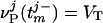; 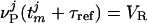, where τ_ref is the refractory period. Here, the membrane potentials of the excitatory (E) [inhibitory (I)] neurons are denoted by , where the superscript j = (j₁, j₂) indexes the spatial location of the neuron within the cortical layer. g_L, g_PE, and g_PI are leaky, excitatory, and inhibitory conductances, respectively. We use normalized, dimensionless potentials with V_I = -2/3, V_T = 1, V_R = 0, and V_E = 14/3 (24).

The time-dependent conductances arise from the input forcing (through the LGN), from “noise” to the layer, and from the cortical network activity of the excitatory and inhibitory populations. They have the general form:

where 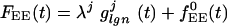, and with similar expressions for , and . S_EE denotes the synaptic strength, a_j-k describes the spatial decay of the coupling, and denotes the temporal time course. The conductance denotes random background forcing, and denotes the forcing from the LGN.

The parameter λ^j ∈ [0, 1] in these equations indicates heuristically how the distribution of simple and complex cells is set in the model and characterizes the simple-complex nature of the jth neuron (with λ^j = 0 the most complex, λ^j = 1 the most simple; models weak cortical excitatory couplings for simple cells), by setting the strength of LGN drive relative to the strength of the cortico-cortical excitation. The parameter λ^j is selected randomly for each neuron, with its distribution determining the distribution of simple and complex cells within the network (21). (Here, only the general structure of the model has been summarized; for a detailed description, see refs. 21, 24, 25.)

Sketch of Derivation of the Kinetic Theory

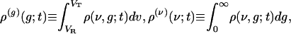
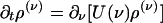
To reduce this large-scale numerical model, we first partition the cortical layer with a tiling of CG patches, with each CG patch sufficiently large to contain hundreds of neurons, yet small enough that the cortical maps and cortical architecture are roughly constant throughout that CG patch. Our goal is to develop an effective description of the dynamics of the neurons within each CG patch. This description is accomplished by kinetic equations that govern the evolution of ρ(ν, g; x, t), the probability density of finding a neuron at time t within the xth CG patch, with voltage ν ∈ (ν, ν + dν) and conductance g ∈ (g, g + dg). For computational efficiency and theoretical analysis, it is of great advantage to further reduce this kinetic theory—a (2 + 1)-D system in the case of single CG patch. A reduction to (1 + 1)-D is achieved by a moment closure.

Next, we sketch this kinetic theory and its closure reduction for a single CG patch. For simplicity, we restrict our description of the derivation to a purely excitatory network containing only α-amino-3-hydroxy-5-methyl-4-isoxazolepropionic acid (AMPA) synapses and simple cells.

The I&F dynamics for the jth neuron in a CG patch of N excitatory neurons is:

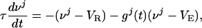[2a]

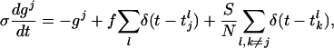[2b]

where τ is the “leakage” time constant, σ is the time constant of the AMPA synapse, f is the synaptic strength from the LGN connections, is the time of the lth LGN spike, is the lth spike time of the kth cortical neuron within the CG patch, and δ(·) is the Dirac delta function. S represents the cortico-cortical coupling strength. We define the pdf by

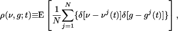[3]

where the expectation E is taken over all realizations of incoming Poisson spike trains from the LGN, and over random initial conditions.

Under the assumptions that (i) N^-1 << 1 and (ii) the summed spike trains to a neuron from many (N) low-rate cortical spike trains (assumed to be independent) is Poisson (26), it can be shown directly from Eq. 2, that ρ(ν, g; t) satisfies the following evolution equation (see refs. 15 and 17 for similar derivations):

[4]

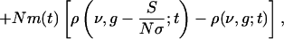where

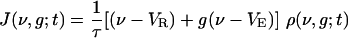is the flux along ν, v₀(t) is the (temporally modulated) rate for the Poisson spike train from the LGN, and m(t) is the population-averaged firing rate per neuron in the CG patch, determined by the J-flux at the threshold to firing:

The (bracketed) discrete differences in g that appear in Eq. 4 arise from the fact that the time course of g after an incoming spike is a single exponential (Eq. 2b). (The theory can be readily generalized to more complicated time courses of conductance.) For small f and large N, these differences can be approximated as derivatives, resulting in

[5]

[6]

To account for the correlation between conductance and voltage in fluctuation dynamics, we investigate the evolution of the marginals and conditional moments:

[7]

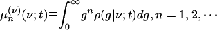where ρ(g|ν; t) is the conditional pdf, i.e., ρ(ν, g; t) = ρ(g|ν;t)ρ^(ν)(ν; t).

Integration of Eq. 5 over ν yields

[8]

which describes the g fluctuations. Under vanishing boundary conditions at g = 0 and as g → ∞, its time-invariant solution can be approximated by a Gaussian. Fig. 2b shows a comparison of this Gaussian approximate solution with a numerical simulation of the original I&F system. Clearly, the reduced Eq. 8 accurately captures the fluctuations in g.

Fig. 2.

Comparison of predictions of the kinetic theory (Eq. 10) with those of full numerical simulation of the I&F network for a single CG patch with N = 300 neurons with the probability of connection between any two cells being 0.25, all excitatory, simple type (σ = 5 ms, τ = 20 ms, S = 0.05, f = 0.01). (a and b)ρ^(ν) (ν) and ρ^(g) (g), respectively. Solid curves are from I&F simulations and circles from kinetic theory. (c) The average population firing rates per neuron, m,as a function of the average input conductance, G_input for σ = 5 ms (dashed) and σ = 0 ms (dash-dotted). (See also refs. 3, 5, and 23.)

Integrating Eq. 5 (and g times Eq. 5) with respect to g yields equations for the marginal ρ^(ν) (and the first moment ):

[9a]

[9b]

where 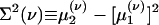is the conditional variance and . Eqs. 9a and 9b are not closed because the equation for the first moment depends on the second moment . Closure is achieved through the assumptions (5): 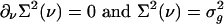, yielding a closed pair of (1 + 1)-D kinetic equations for ρ^(ν) (ν; t) and (ν; t):

[10a]

[10b]

These kinetic equations are solved for V_R ≤ ν ≤ V_T, under two-point boundary conditions in ν, which are derived from the fact that the flux J(ν, g) across firing threshold V_T is equal to the flux at reset V_R, adjusted for a finite refractory period. This reduction in dimension from (2 + 1)-D to (1 + 1)-D yields a significant computational savings in addition to the savings achieved by the pdf representation itself (see below).

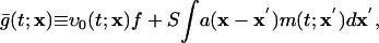
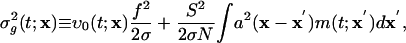
This derivation extends to more realistic networks containing excitatory and inhibitory neurons of both simple and complex types, with AMPA excitatory synapses, and with coupling between many CG patches. Results in the next section are for such networks. Coupling between CG patches is accomplished by replacing Eq. 6 with

[11a]

[11b]

where x denotes the coarse-grained spatial label and a(x) described a smoothed network coupling a_ij.

We note that, because the AMPA timescale σ is much smaller than the leakage timescale τ, a further reduction could be achieved by coarse-graining in time, resulting in an effective dynamics, which might be useful for analytical insight. (However, it turns out to be not very accurate quantitatively, as can be seen below.) The case of σ = 0 has been considered in the literature (see, e.g., refs. 13, 17, 23, and 27). Here, as the limit σ → 0, recalling that , Eq. 10b reduces to , which on insertion into Eq. 10a yields a closed equation for ρ^(ν) (ν; t) only:

[12]

where . We can show that this Fokker–Planck equation is consistent with a white-noise limit of the underlying stochastic processes of conductance. Notice that, as the number of neurons in the CG patch N → ∞ and f → 0, then ; thus, the fluctuations drop out of Eq. 12, and the dynamics reduces to “mean-driven” dynamics (3, 9, 18, 23).

Results

We now compare this kinetic theory with full numerical simulations of an I&F network. We find that it is surprisingly accurate, as clearly illustrated in Fig. 2. We emphasize that there are no adjustable free parameters in these comparisons. Two additional points are worth noting: (i) At small average input conductance G_input = v₀f, a regime in which fluctuations dominate, the mean-driven theory (N → ∞, f → 0) does not at all capture the population response; (ii) Had we used the diffusion limit, i.e., Eq. 12, we would not be able to achieve nearly the same accuracy (see the dash-dotted line in Fig. 2) for physiological values of σ.

We further illustrate the effectiveness of the kinetic dynamics in describing fluctuation-driven behavior by considering a yet smaller network of only N = 16 excitatory cells with relatively strong cortico-cortical connections. For this small N, the network is very much fluctuation-driven. The dynamics of this excitatory network exhibits bistability with a sharp transition as the average input conductance G_input is increased.¶ Fig. 3 shows the bifurcation diagram for the firing rate m as a function of G_input. The theoretical prediction of the kinetic theory is compared with those of numerical simulation. The agreement is again extremely good, even for such a small number of neurons. Again, we note that the mean-driven theory (dotted line) does not correctly predict the location of switch-up of the bifurcation diagram.

Fig. 3.

Bifurcation diagrams for the firing rate m versus average input conductance G_input, which compare numerical simulation results with the prediction of the kinetic theory (Eq. 10 in the small σ-limit), for a CG patch containing a small number (N = 16) of excitatory neurons with all-to-all connections (σ = 5 ms, S = 0.45, τ_ref = 3 ms). Theory (thick dashed line) shows lower and upper branches in the bistable region, with a sharp transition from A to B. Simulation results are obtained by slowly “ramping” G_input, first up, then down. Arrows indicate the results of the simulations with respect to ramping G_input up and down. (Inset) The transition region for the branch moving up from A to B only, for different realizations of input Poisson spikes. Dotted line (with a jump at G_input ∼ 13.5) is the prediction of the mean-driven theory.

As expected in refs. 5, 22, and 28, in addition to having accuracy, the kinetic representation (Eq. 10) is far more efficient computationally than the full I&F network. The reduction is 2-fold: (i) the pdf representation yields a great computational savings by eliminating the need of running either for very long times or for many ensembles of the same I&F network to reduce the statistical error in computing firing rates; (ii) The reduction from the (2 + 1)-D systems (Eq. 4) to the (1 + 1)-D PDEs (Eq. 10) provides really significant savings. For example, to achieve a rate computation within 1% accuracy for a network of 100 neurons, a reduction of 3–4 orders of magnitude in computation work can be easily obtained.

Next, and for the remainder of this section, we turn to a neuronal network containing hundreds of neurons (75% excitatory and 25% inhibitory) with equal proportions of simple and complex cells. Here, simple and complex cells are modeled by the following network architecture: Simple cells are driven externally, in addition to their inputs from all other cells, whereas complex cells receive inputs only from all other cells and are not driven externally. The network is modeled by four coupled kinetic equations of excitatory/inhibitory simple and complex populations. We emphasize that here the inhibitory population also fully incorporates fluctuations. Fig. 4 shows the firing rate diagrams (m vs. G_input) for the two excitatory populations, one simple and one complex, as predicted by our kinetic theory. Also shown is the large-N, mean-driven limit, whose bifurcation diagram shows a complicated bistable, hysteretic structure, as the simple and complex neuronal types jump together between their respective lower and upper branches. This structure is in marked contrast to the small-N network limit. It is important to note that for the network with this particular cortical connection strength, the fluctuations are so strong any apparent sharp bifurcation/hysteresis no longer exists in the small-N case.

Fig. 4.

Bifurcation diagrams for excitatory firing rate m versus average input conductance G_input predicted by the kinetic theory for a network, 1/2 of which are simple and 1/2 of which are complex, and 3/4(1/4) of which are excitatory (inhibitory). The large figure displays the large-N limit, and the inset is the finite (N = 75) fluctuation-driven result; in each case, firing curves are shown for both simple (dotted or dash-dotted) and complex excitatory (dash or solid) cells. Note the complicated structure of the mean-driven (N → ∞) case, which results from an interplay between the bifurcations of the simple and complex cells. In more detail: at point A, simple cells reach firing threshold in terms of G_inp, and begin to fire. With increasing G_inp, the firing curve follows A → D → B. At the same time, because of the increasing input from the simple cells, the complex cells reach firing threshold at point B′ in terms of G_inp and abruptly jump from zero firing rate to point C′. Because of this jump, the firing rate of simple cells jumps from B to C. If G_inp is decreased, the firing curve of complex cells follows C′ → D′ and shut off at D′, whereas the simple cells follow the corresponding firing curve, starting from C and revisiting D. With G_inp further decreasing, the simple cells trace the firing curve AD backward to point A and then shut off. The complex cells exhibit a hysteretic loop D′B′C′D′, associated with the hysteretic loop DBCD for the simple cells. (Inset) The much simplified firing-rate diagram for the finite population, fluctuation-driven kinetic theory for the network at this particular cortico-cortical connection strength.

Fig. 5 shows firing rate m vs. G_input relations for three different values of cortico-cortical excitation strength for complex neurons in a network containing both excitatory and inhibitory neurons of both simple and complex type. These response diagrams compare the predictions of the kinetic theory (in the small-σ limit) with those computed by numerical simulations of an I&F network and display good qualitative agreement: Fig. 5a shows the theoretical results for excitatory neurons, one simple and one complex, whereas Fig. 5b shows the same results computed by simulation. As is increased, these response curves change from no bistability/hysteresis, through critical response, to bistability/hysteresis at strong .

Fig. 5.

Bifurcation diagrams. Excitatory firing rate m versus average input conductance G_input for a neuronal network with random connectivity, containing 400 I&F neurons, 1/2 of which are simple and 1/2 of which are complex, and 3/4 (1/4) of which are excitatory (inhibitory) with the probability of connection between any two cells being 0.25. (a) Prediction of our kinetic theory. (b) Results from numerical simulation of the I&F network. The figures show results for simple (light lines) and complex (heavy lines) excitatory neurons, for three increasing values of the coupling strengths, , of cortico-cortical excitation for complex type. The theoretical results in a show a steepening of the curves as is increased, from monotonic, through critical, to bistable. The corresponding simulation results (b) show the same behavior with the bistability being manifested in the hysteresis (with transitions indicated by arrows).

Discussion

These results suggest to us that, depending on cortical connection strength, complex cells that are well selective for orientation may be the result of the network response moving across the critical region of “near-bistability.” Here, we describe some further evidence in this direction from a kinetic theory for “ring models” (16) as one example of the utility of kinetic theory for insight into possible cortical mechanism.

We use our large-scale I&F model of input layer 4Cα (21, 24, 25), to motivate a family of idealized I&F “ring models,” indexed by the radius of the ring measured from a pinwheel center. As discussed above these I&F networks consist of 75%/25% excitatory/inhibitory neurons with the coupling range of inhibitory neurons shorter than that of excitatory neurons. The simple cells are all driven by the LGN, but with weak cortico-cortical excitation, whereas the complex cells, which receive no LGN drive, have stronger cortico-cortical excitation. This simple/complex architecture is shown schematically in Fig. 1a. These ring models are idealizations of the large-scale network, with the I&F neurons restricted to reside on a circle centered on an orientation pinwheel center (see the white circle in Fig. 1b) (16, 17, 29). In the models, the cortico-cortical coupling strengths are Gaussians falling off with distance between the neurons—cortical distance in the case of the large-scale model and angular distance in the ring models. The radius of the ring is used to convert the cortical coupling lengths of neurons in the large-scale model to coupling lengths in the angle γ along the ring, with broad coupling lengths in γ for rings of small radii (whose neurons reside close to the pinwheel center), and narrow lengths in γ for rings of large radii (whose neurons reside far from the pinwheel center).

We drive these models with drifting gratings set at an angle of orientation θ. Fig. 6 shows orientation tuning curves [firing rate m(θ)] for simple (dashed) and complex (solid) cells in two different ring models, both far from the pinwheel center, but one with weak fluctuations (Fig. 6a) and the other with stronger fluctuations (Fig. 6b) (achieved by removing slow N-methyl-d-aspartate (NMDA) excitatory synapses from the network while keeping the cortico-cortical coupling strength the same.) Note the tuning curves shown in Fig. 6a display the characteristics of a mean-driven, high-conductance (30) state with weak fluctuations being driven across the bifurcation point—characteristics identified through use of the kinetic representations: very high firing rates of the complex cell, together with the very low firing rates of the simple cell; very sharp transitions (in θ) in the firing rate of the complex cell; and a strong synchrony in the firing patterns of the complex cells (as shown in the raster plot inset). On the other hand, the tuning curves of Fig. 6b display the characteristics of a fluctuation-driven state: more reasonable firing rates; a more gradual behavior as a function of θ; and the lack of synchrony in the firing patterns of the complex cells (again shown in the raster plot inset).

Fig. 6.

Orientation tuning curves for a ring model containing excitatory and inhibitory neurons of both simple (dashed) and complex (solid) type, computed from numerical simulations of an I&F network. (a) A mean-driven state with negligible fluctuations. Note the characteristics of a mean-driven, high-conductance state: abnormally high firing rates in the complex cell, together with the very low firing rates of the simple cell; the sharp transition in the firing rate of the complex cell as a function of θ; and the strong synchrony in the firing patterns of the complex cells (as shown in the raster plot inset). (b) A fluctuation-driven state. Note the more reasonable firing rates, their more gradual behavior as a function of θ, and the absence of synchrony in the firing patterns of the complex cells (again shown in the raster plot inset).

Fig. 7 shows results for two ring models [one with a small radius (Fig. 7 a and d), which is near the pinwheel center, and one with a larger radius (Fig. 7 b and e), which is far from the pinwheel center]; together with results for the full large-scale 1 mm² network (Fig. 7 c and f). Fig. 7 a–c shows orientation tuning curves, i.e., m(θ), whereas Fig. 7 d–f shows response diagrams (firing rate m vs. the strength of the conductance drive). The samples shown are complex cells. In the response diagrams, heavy bold curves show behavior as the driving strength is increased, whereas regular curves depict responses as driving strength is decreased. The dashed lines in Fig. 7 a and b depicts the results from the kinetic theory extended to the ring model with excitatory, inhibitory, simple, and complex neurons. In this extension, the kinetic equations for the coarse-grained patches are coupled according to Eq. 11, with the angular variable θ replacing the spatial variable x as the labeling of the CG patches in the ring model.

Fig. 7.

Comparison of the firing rate behavior under drifting grating stimuli of three neuronal networks, two ring models and a large-scale I&F 1 mm² model (21). Each model contains 75% (25%) excitatory (inhibitory) neurons and simple and complex cells. For sample complex neurons, a–c show orientation-tuning curves (firing rate m(θ), where θ denotes the orientation of the drifting grating), comparing the results of the full I&F networks (solid line) with those of the kinetic theory (dashed line); whereas d–f show response diagrams (m(θ) vs. the driving strength). In these response diagrams, heavy bold curves show behavior during “switch-up” of the driving strength, and regular curves depict responses to “switch-down.” (a and d) A ring model of small radius (with neurons near the pinwheel center). (b and e) A ring model of large radius (far from pinwheel center). (c and f) A neuron from the large-scale model that is far from any pinwheel center.

Note that (i) each of these three networks is operating in a fluctuation-driven regime; (ii) for the ring of small radius (Fig. 7d), the firing rates rise gradually with increasing driving strength; (iii) the opposite is true for the ring of large radius, which has a much steeper dependence of firing rate on driving strength (Fig. 7e). This behavior, together with that of the orientation-tuning curves (Fig. 7 a and b), provides a strong indication that those complex cells that are quite selective for orientation might result from operating at or near a critical transition. We (21) have yet to construct a large-scale network that operates realistically in this regime, primarily because, as the regime is approached, instabilities in the network appear and cause synchronization of the neurons that is reminiscent of the mean-driven state with small fluctuations.

The kinetic theory described here clearly provides theoretical insight into possible cortical mechanisms in fluctuation-dominated systems. It also provides an efficient and remarkably accurate computational method for numerical studies of very-large-scale neuronal networks. More detailed studies, using this kinetic theory, of large-scale networks of simple and complex cells will be published elsewhere.

References

- 1.Anderson, J., Lampl, I., Gillespie, D. & Ferster, D. (2000) Science 290, 1968-1972. [DOI] [PubMed] [Google Scholar]
- 2.Stern, E., Kincaid, A. & Wilson, C. (1997) J. Neurophysiol. 77, 1697-1715. [DOI] [PubMed] [Google Scholar]
- 3.Shelley, M. & McLaughlin, D. (2002) J. Comput. Neurosci. 12, 97-122. [DOI] [PubMed] [Google Scholar]
- 4.Fourcaud, N. & Brunel, N. (2002) Neural Comput. 14, 2057-2110. [DOI] [PubMed] [Google Scholar]
- 5.Haskell, E., Nykamp, D. & Tranchina, D. (2001) Network: Comput. Neural, Syst. 12, 141-174. [PubMed] [Google Scholar]
- 6.Knight, B. (1972) J. Gen. Physiol. 59, 734-766. [DOI] [PMC free article] [PubMed] [Google Scholar]
- 7.Wilbur, W. & Rinzel, J. (1983) J. Theor. Biol. 105, 345-368. [DOI] [PubMed] [Google Scholar]
- 8.Abbott, L. & van Vreeswijk, C. (1993) Phys. Rev. E 48, 1483-1490. [DOI] [PubMed] [Google Scholar]
- 9.Treves, A. (1993) Network 4, 259-284. [Google Scholar]
- 10.Chawanya, T., Aoyagi, A., Nishikawa, T., Okuda, K. & Kuramoto, Y. (1993) Biol. Cybern. 68, 483-490. [DOI] [PubMed] [Google Scholar]
- 11.Barna, G., Grobler, T. & Erdi, P. (1998) Biol. Cybern. 79, 309-321. [DOI] [PubMed] [Google Scholar]
- 12.Pham, J., Pakdaman, K., Champagnat, J. & Vibert, J. (1998) Neural Networks 11, 415-434. [DOI] [PubMed] [Google Scholar]
- 13.Brunel, N. & Hakim, V. (1999) Neural Comput. 11, 1621-1671. [DOI] [PubMed] [Google Scholar]
- 14.Gerstner, W. (2000) Neural Comput. 12, 43-80. [DOI] [PubMed] [Google Scholar]
- 15.Omurtag, A., Knight, B. & Sirovich, L. (2000) J. Comput. Neurosci. 8, 51-63. [DOI] [PubMed] [Google Scholar]
- 16.Omurtag, A., Kaplan, E., Knight, B. & Sirovich, L. (2000) Network: Comput. Neural. Syst. 11, 247-260. [PubMed] [Google Scholar]
- 17.Nykamp, D. & Tranchina, D. (2000) J. Comput. Neurosci. 8, 19-50. [DOI] [PubMed] [Google Scholar]
- 18.Nykamp, D. & Tranchina, D. (2001) Neural Comput. 13, 511-546. [DOI] [PubMed] [Google Scholar]
- 19.Hubel, D. & Wiesel, T. (1962) J. Physiol. (London) 160, 106-154. [DOI] [PMC free article] [PubMed] [Google Scholar]
- 20.Chance, F., Nelson, S. & Abbott, L. (1999) Nat. Neurosci. 2, 277-282. [DOI] [PubMed] [Google Scholar]
- 21.Tao, L., Shelley, M., McLaughlin, D. & Shapley, R. (2004) Proc. Natl. Acad. Sci. USA 101, 366-371. [DOI] [PMC free article] [PubMed] [Google Scholar]
- 22.Knight, B., Manin, D. & Sirovich, L. (1996) in Symposium on Robotics and Cybernetics: Computational Engineering in Systems Applications, ed. Gerf, E. (Cite Scientifique, Lille, France), pp. 185-189.
- 23.Sirovich, L., Omurtag, A. & Knight, B. (2000) SIAM J. Appl. Math. 60, 2009-2028. [Google Scholar]
- 24.McLaughlin, D., Shapley, R., Shelley, M. & Wielaard, J. (2000) Proc. Natl. Acad. Sci. USA 97, 8087-8092. [DOI] [PMC free article] [PubMed] [Google Scholar]
- 25.Wielaard, J., Shelley, M., Shapley, R. & McLaughlin, D. (2001) J. Neurosci. 21, 5203-5211. [DOI] [PMC free article] [PubMed] [Google Scholar]
- 26.Cinlar, E. (1972) in Stochastic Point Processes: Statistical Analysis, Theory, and Applications, ed. Lewis, P. (Wiley, New York), pp. 549-606.
- 27.Knight, B. (2000) Neural Comput. 12, 473-518. [DOI] [PubMed] [Google Scholar]
- 28.Casti, A., Omurtag, A., Sornborger, A., Kaplan, E., Knight, B., Victor, J. & Sirovich, L. (2002) Neural Comput. 14, 957-986. [DOI] [PubMed] [Google Scholar]
- 29.Somers, D., Nelson, S. & Sur, M. (1995) J. Neurosci. 15, 5448-5465. [DOI] [PMC free article] [PubMed] [Google Scholar]
- 30.Shelley, M., McLaughlin, D., Shapley, R. & Wielaard, J. (2002) J. Comput. Neurosci. 13, 93-109. [DOI] [PubMed] [Google Scholar]
- 31.Blasdel, G. (1992) J. Neurosci. 12, 3115-3138. [DOI] [PMC free article] [PubMed] [Google Scholar]
- 32.Blasdel, G. (1992) J. Neurosci. 12, 3139-3161. [DOI] [PMC free article] [PubMed] [Google Scholar]