

Abstract
We present a methodological framework for multichannel Markov random fields (MRFs). We show that conditional independence allows loopy belief propagation to solve a multichannel MRF as a single channel MRF. We use conditional mutual information to search for features that satisfy conditional independence assumptions. Using this framework we incorporate kinetic feature maps derived from breast dynamic contrast enhanced magnetic resonance imaging as observation channels in MRF for tumor segmentation. Our algorithm based on multichannel MRF achieves an receiver operating characteristic area under curve (AUC) of 0.97 for tumor segmentation when using a radiologist's manual delineation as ground truth. Single channel MRF based on the best feature chosen from the same pool of features as used by the multichannel MRF achieved a lower AUC of 0.89. We also present a comparison against the well established normalized cuts segmentation algorithm along with commonly used approaches for breast tumor segmentation including fuzzy C-means (FCM) and the more recent method of running FCM on enhancement variance features (FCM-VES). These previous methods give a lower AUC of 0.92, 0.88, and 0.60, respectively. Finally, we also investigate the role of superior segmentation in feature extraction and tumor characterization. Specifically, we examine the effect of improved segmentation on predicting the probability of breast cancer recurrence as determined by a validated tumor gene expression assay. We demonstrate that an support vector machine classifier trained on kinetic statistics extracted from tumors as segmented by our algorithm gives a significant improvement in distinguishing between women with high and low recurrence risk, giving an AUC of 0.88 as compared to 0.79, 0.76, 0.75, and 0.66 when using normalized cuts, single channel MRF, FCM, and FCM-VES, respectively, for segmentation.
Index Terms: Breast cancer recurrence prediction, breast dynamic contrast enhanced (DCE) magnetic resonance imaging (MRI), breast tumor segmentation, tumor characterization
I. Introduction
Crucial to the performance of a feature extraction and image classification system is the availability of a reliable and accurate segmentation approach for the object of interest (e.g., tumor). In most medical imaging applications, the automation of this step is particularly important because of the large amount of images to be analyzed. This makes the manual segmentation approach tedious and prohibitively expensive. As a result, extensive research has been done in the medical imaging community for improving the quality of automated segmentation. Specifically, there is an abundance of methods geared towards segmenting well defined anatomical structures (e.g., parts of the brain). Notable among them are the variants of active contours [1] and active shape models [2]. There are two main drawbacks associated with this class of methods. First, they require manual initialization that should be very close to the actual structure to be segmented. Efforts for automating the initialization step have been restricted to structures for which precise a priori knowledge is available [3]. Second, they aim at segmenting known anatomical structures that have well defined control points in their shape, which is often not the case for arbitrarily shaped lesions. Fuzzy C means (FCM) clustering and its variants are also prevalent for the segmentation of well defined structures [4]–[6]. Markov random field (MRF) based approaches have also been used for segmentation. For instance, in [7], the authors model brain magnetic resonance imaging (MRI) images as a MRF and use prior information for segmenting anatomical structures. Another approach for segmentation includes spectral graph clustering methods [8]–[10]. Notable among them is the normalized cuts algorithm [8] which is a highly robust segmentation method and is widely used for segmentation applications [11]–[14]. Specifically, [11] uses normalized cuts for MRI image segmentation.
As compared to anatomically well defined structures, there is relatively less work in the literature on segmenting arbitrarily shaped structures (e.g., breast tumors). Among the work done on breast tumor segmentation the most popular approach is FCM clustering employed by many researchers due to its simplicity (e.g., [15], [16]). More recently Lee et al. [17] presented a method that runs FCM on the variance map of enhancement kinetics (FCM-VES). Although useful for segmentation, these methods do not take into account the overlap of the feature values of the tumor and nontumor pixels. As a result they have to settle with a manually set threshold on FCM membership probabilities, leading to poor generalization. In order to address these issues we propose to incorporate a component of learning for breast tumor segmentation. We present a framework for multichannel extension of MRFs to make maximal usage of multiple feature streams derived from the imaging data, here specifically related to kinetic analysis of dynamic contrast enhanced (DCE) breast MR images.
We have previously shown that a multichannel extension of MRFs is feasible [18]. In this paper, we present a complete methodological framework, selection of conditionally independent feature channels for MRF, extended comparison with other segmentation algorithms, and assessment of the potential impact of improved segmentation on classification and characterization of breast cancer tumors. We explore how inference methods like loopy belief propagation [19] may be extended for a multichannel MRF. There have been considerable work in the literature that uses MRF for segmentation. In a representative work [7], authors address the problem of brain image segmentation using MRFs and present an expectation maximization framework to solve the MRF. However, the approach in [7] is limited to a single channel MRF. Often, it is desirable to integrate information from different channels, if available, to achieve better segmentation. For example, in our specific application, multiple channels would allow to take maximum advantage of DCE MRI kinetic features that represent the properties of contrast agent uptake by the tissue, which are expected to be different for tumor and background tissues [15], [20]. In this work we exploit conditional independence for solving an MRF via loopy belief propagation [19] that reduces a multichannel MRF to a single channel MRF for inference queries, allowing to capitalize on information coming in from different channels. We also present a principled method to choose features satisfying conditional independence to be included as multiple channels in the MRF observation model.
Key contributions of this paper are as follows.
We show that conditional independence allows loopy belief propagation to solve a multichannel MRF as a single channel MRF thereby avoiding the modeling of joint distributions (Section II).
Using conditional mutual information we present a principled method for choosing conditionally independent features as different channels in the MRF observation model (Section III).
To elaborate on this premise, we introduce multiple feature channels derived from the kinetic analysis of DCE magnetic resonance (MR) images in the observation model of MRF (Section III).
We show that our segmentation algorithm yields an area under curve (AUC) of 0.97 under the ROC curve for breast tumor segmentation compared to 0.89 for single channel MRF using the best feature from the same pool of features as used by our multichannel MRF. Also, the normalized cuts segmentation algorithm and commonly used approaches for breast tumor segmentation, [15], [17] gave lower AUCs (0.92, 0.88, and 0.60) (Section IV).
Finally we demonstrate that superior segmentation leads to improved feature extraction and tumor characterization. In the specific application presented here, we show that our segmentation method leads to improvement in image-based prediction of breast cancer prognosis by distinguishing between patients with high and low recurrence risks as determined by a validated gene expression assay (Section V).
II. Multichannel MRF
To elaborate on the MRF concept, Fig. 1 shows how an image can be modeled as a MRF. Each node (X) represents the class of a pixel, and neighboring pixels are connected via edges. In the context of segmentation the goal is to infer the class label for each pixel (e.g., foreground versus background). For a detailed review on single channel MRFs see [21]. Here, we present a multichannel extension of MRFs and elaborate how to incorporate multiple observations in the MRF model. In Fig. 1 each node emits two observations, Y and W (similar notion could be extended to more than two observations). The joint probability of the pixel class and the two observations over the entire image is given below
Fig. 1.

Multichannel MRF with two observations for each node. The variables inscribed in the triangle represent the joint distribution of the MRF model. If the observation variables (Y, W) are conditionally independent given the hidden variable (X), the joint distribution can be factorized into two parts, represented by ellipses, allowing loopy belief propagation to solve a multichannel MRF as a single channel MRF (see Section II).
| (1) |
where
| (2) |
| (3) |
In (1), ϕi(ℳ
 ) is the multichannel node potential for the two observations, and ψ represents the edge potential, and E models the adjacency of nodes including only those nodes that have edges between them. The node potential captures the correlation between the features and the class label, indicating the likelihood of xi coming from class c based on the feature values of yi, wi and the feature distribution of class c. In (3), ℐ(xi ≠ xj) is an indicator function that equals 1 when xi ≠ xj and 0 otherwise. As a result, ψ biases neighboring nodes to have the same class label via the parameter β. In (2),
 ℳℳc is a Gaussian mixture model learned for class c for features y, w which can be learned from labeled training data. It is clear from (2) that with increasing number of observations the task of modeling the node potential as a joint distribution would become difficult. However, if the features in different channels are conditionally independent given the hidden variable (X), we can factorize the right-hand side of (2) as follows:
| (4) |
Equivalently (4) can be written as
| (5) |
where and are the individual node potentials for the features y and w respectively, which can be learned from labeled training data (see Section III-D). The individual node potentials, and , can be multiplied together to give a single potential representing the multichannel potential. In Section III-C, we present a principled method to choose features satisfying conditional independence to invoke the factorization given in (4). Using (4) the inference machinery for solving a single channel MRF can be reused for multichannel MRFs as well, described below.
A. Inference in Multichannel MRFs
Inference in the above mentioned MRF involves the maximum a posteriori (MAP) estimate of the state of each node in the MRF. For tree structured distributions, the MAP estimate for the random fields can be computed efficiently by dynamic programming [22]. If the graphical model is a tree it can also be computed in polynomial time using graph cuts [23]. For more general settings, the belief propagation (BP) algorithm is an efficient way for solving inference problems in graphical models [24]. Specifically, in [24], the authors show that the fixed points arrived at by the BP algorithm correspond to the Bethe approximation of the free energy of a factor graph. Moreover, minimizing the free energy in turn corresponds to minimizing the Kullback–Leibler divergence between a “trial” distribution and the distribution that needs to be recovered [24], [25]. As such belief propagation offers an efficient solution toward estimating inference probabilities in graphical models. It should be noted that the BP algorithm solves inference problems exactly when the factor graph is a tree, and only approximately when the graph has cycles [24]. There are BP algorithms that give good approximate results even for graphical models with cycles [24]. If the graph has cycles, the corresponding BP algorithm is often referred to as “loopy” belief propagation [19]. Freeman et al. [24] present a seminal description as to why BP algorithm works well which is primarily due to its equivalence with minimizing the free energy of the factor graph, thereby arriving at better approximation of the distribution that needs to be recovered. As such, the BP algorithm has significant advantages over other inference methods, [19], [24], [25].
To capitalize on the advantages of the BP algorithm we investigate the loopy belief propagation algorithm to solve our multichannel MRF. Loopy BP is a dynamic message passing algorithm used for doing inference in MRF. δi→j (
 j) is defined to be an incoming message into node j from its neighboring node i. Intuitively, δi→j captures the degree of belief that node i has about node j. To start the process of message passing through the nodes, the node messages are initialized (typically to unity) and then the messages can be updated in the next iteration as follows:
| (6) |
where Zi→j is a normalization constant, and
 (i) is a set containing the neighbors of node i. Equation (6) is repeatedly invoked till the messages converge (the update in each message is less than ∊ e.g., 10−6). Once the messages have converged the final inference is done by using
| (7) |
The inference engine will output for each node a vector of size C × 1 (C = 2 for two classes), representing the belief of this node coming from each class. Optimal class label is simply the class with the highest belief.
In the next section, we elaborate on the extraction of pixel-wise feature maps to build a kinetic observation model for our multichannel MRF.
III. Multichannel MRF Based on DCE-MRI Kinetics
A. Candidate Feature Channels
Typically, for DCE MR images we have a precontrast image (captured prior to the injection of a contrast agent) and a number of postcontrast images, captured at different time points after the injection of the contrast agent [20]. The uptake of the contrast agent by different tissues manifests itself in the form of contrast enhancement in postcontrast MR images, and the enhancement patterns, in general, are different for tumor and background tissues [26], [15]. As such DCE MRI derived features hold promise for differentiating between tumor and background tissues and we propose to investigate them as candidate features for our multichannel MRF observation model.
A common way to quantify the enhancement pattern is to compute relative enhancements as compared to the precontrast image [17], [20]. By computing the relative enhancement on a pixel by pixel basis we can construct pixel wise maps of the relative contrast enhancement as follows:
| (8) |
where I(u, v, t) represents the intensity of pixel (u, v) captured at time t, and t0 is the precontrast time instant. For a particular pixel, the relative enhancement plotted as a function of time is defined as the kinetic curve [20]. In the literature (e.g., [17], [20]) a number of basic features can be computed from this kinetic curve as illustrated in Fig. 2(a). Based on these features we can derive a rich kinetic feature set by computing the pixel-wise map for each feature as follows.
Fig. 2.

Candidate features for different observation channels of our multichannel MRF. (a) Illustration of basic kinetic features for a single pixel. (b) Pixel wise maps of enhancement for three postcontrast time points. (c) Pixel wise maps of kinetic features: peak enhancement (
 ℰ), wash-in-slope (
 ), wash-out-slope (
 ).
).
-
Peak enhancement (ℰ)
(9) which represents the peak relative enhancement for every pixel as computed over all postcontrast time points.
-
Time to peak (
 )
)
(10) which represents the time at which peak enhancement is achieved.
-
Wash-in slope ()
(11) which is a measure of the initial uptake rate of the contrast agent for every pixel.
-
Wash-out slope ()
(12) where tM is the last postcontrast time instant. The wash-out slope captures the drop in the uptake rate of the contrast agent after the peak enhancement is achieved.
Example pixel-wise maps of above features are depicted in Fig. 2(b). For the rest of the paper we use ℰi to represent the relative enhancement map for the ith postcontrast time point. We investigate the utility of these feature maps when included in our multichannel MRF observation model for the purpose of breast tumor segmentation.
B. MRF Representation-Superpixels
Many computer vision algorithms use the pixel grid as an underlying representation. MRFs are also often defined on this regular grid. The pixel grid, however is not a natural representation of the imaged structure, but rather an artefact of the imaging process [27]. As a result there has been significant work in deriving efficient and perceptually meaningful entities from a low level grouping process [27]–[29]. A popular approach is to divide the image into segments of homogeneity called superpixels [8]. Following the approach in [8], we first over-segmented the DCE MR images into superpixels. There are a number of advantages to defining the MRF over the superpixels rather than individual pixels. First, it reduces the complexity of images to a few hundred pixels. Second, they are representationally efficient in that they allow longer range interactions between superpixels, which in the case of a regular grid are restricted to adjacent pixels in the grid [28]. In order to define the MRF neighborhood for superpixels we scan the rows and columns of the superpixelized image and look for transitions. This enables to build the adjacency matrix for superpixels that captures the neighborhood. An example of the oversegmentation step using superpixels is shown in Fig. 3. For this step, we used the publicly available implementation1 of superpixels based on [28], [29]. Throughout this work the input image was first segmented into 100 superpixels that were used as nodes in the MRF. If is the number of MRF nodes, the per-iteration complexity of loopy belief propagation message update (6) ranges from O(N) to O(N2), depending on the connectedness of the nodes in the graph. As such defining the MRF over superpixels greatly reduces the complexity of the message update step.
Fig. 3.
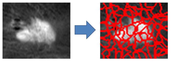
Illustration of the oversegmentation step using superpixels. Here an image consisting of ∼ 5000 pixels has been divided into 100 superpixels.
C. Feature Choice for Multichannel MRF
The multichannel MRF described in Section II is based on features that are conditionally independent of one another given the pixel class. It is well known that mutual information is a good indicator of statistical dependence (or lack thereof) between random variables [30]. Small values of mutual information between two random variables indicate little statistical dependence between the two. When certain variables are known, the conditional mutual information captures the influence of this knowledge on the statistical interaction between the variables in question. We thus use conditional mutual information as a criterion to assess the conditional independence of our features. Specifically, in the multichannel MRF of Fig. 1, we are interested in assessing the independence of Y and W given X. Their conditional mutual information is given by
| (13) |
The variable X represents the class of the pixel and hence is discrete, whereas the features represented by Y and W are continuous. To compute the distributions required for evaluating the above mutual information, one option is to discretize the continuous variables and use histograms as approximation to the probability densities. However, the inefficiencies of histograms for modeling probability densities, especially the inherent discontinuities, are well recognized in the literature [31]–[33]. Therefore we employed kernel density estimation [32], [34] for estimating the densities required for computing the mutual information. For all computations, the Gaussian kernel was used. For bandwidth selection, a data driven approach for computing diagonal bandwidth matrix for multivariate Gaussian kernel was employed [34].
We computed I(Y; W∣X) by sequentially setting (Y, W) to all possible pairs of the following six feature maps: postcontrast enhancements (ℰ1, ℰ2, ℰ3), peak enhancement (
ℰ), wash-in-slope (
), and wash-out-slope (
). The features with the least conditional mutual information were selected as channels for the multichannel MRF (see Section IV-B).
D. Training-Learning Node Potentials
The training step involves the computation of node potentials as given in (5). We model node potentials as a mixture of Gaussian distributions. A Gaussian mixture model (
ℳℳ) is a weighted sum of M component Gaussian distributions [35]. For example, we can express the node potential for feature y as follows:
| (14) |
where
ℳℳc represents the Gaussian mixture model for class c (e.g., tumor and nontumor pixels), wr is the weight of the rth Gaussian component specified by the respective mean and variance parameters, μr and
.
represents the Gaussian pdf with the respective parameters as follows:
| (15) |
At training step we need to learn the following parameters for class c:
| (16) |
There are several techniques available for estimating the parameters of a
ℳℳ [35]. A popular approach for estimating these parameters is through an iterative maximum likelihood estimation using the expectation maximization (EM) algorithm [36]. For learning the node potentials for our multichannel MRF we employed the EM algorithm based method (Matlab statistics toolbox2) and used M = 5 Gaussian components. To enable maximal usage of the training data we used a leave-one-out cross validation strategy for computing node potentials. For every test image, the rest of the data was considered as training set and node potentials were computed using the training set.
IV. Segmentation Experiments
A. Dataset
All experiments presented in this paper were conducted on DCE breast MR images of 60 women diagnosed with breast cancer. The dataset consists of bilateral breast MRI sagittal scans collected at our institution from 2007–2010. The ages of the women at the time of the imaging ranged from 37 to 74 years with a mean age of 55.5 years. Of the women analyzed, 93% had their primary tumor classified as T1 i.e., the tumor was 2.0 cm or less in the greatest dimension (GD). The rest of the primary tumors were T2 (2 cm < GD ≤ 5 cm). Within the T1 tumors the distribution was as follows: 8%(0.1 cm < GD ≤ 0.5 cm); 37% (0.5 cm < GD ≤ 1 cm); 45% (1 cm < GD ≤ 2 cm). The imaging protocol is as follows: The women were imaged prone in a 1.5T scanner (GE LX echo, GE Healthcare, or Siemens Sonata, Siemens); matrix size: 512 × 512; slice thickness: 2.4–4.4 mm; flip angle: 25° or 30°. The images were collected before and after the administration of gadodiamide (Omniscan) or gadobenate dimeglumine (MultiHance) contrast agents. Dynamic contrast enhanced images were acquired at 90-s intervals for three postcontrast time points.
The women in the dataset had estrogen receptor positive (ER+), node negative tumors, which were analyzed with the Oncotype DX prognostic gene expression assay [18]. Oncotype DX is a validated reverse-transcriptase-polymerase-chain-reaction (RT-PCR) assay (developed by Genomic Health Inc.) that measures the expression of 21 genes in RNA from formalin-fixed paraffin-embedded (FFPE) tumor tissue samples from the primary breast cancer [37]. The final outcome of the Oncotype DX assay is a continuous recurrence score that predicts the likelihood of breast cancer recurrence in 10 years after the treatment (risk: low ≤ 17%, 18 % < medium > 30% high ≥ 31%). It has been shown that the benefit of adjuvant chemotherapy regimen starts becoming significant only in patients with an Oncotype score greater than 30 [37]. To learn feature statistics for distinguishing the breast tumor and nontumor area of an image, a fellowship-trained board-certified breast imaging radiologist delineated the lesion boundaries using the software ITK-SNAP [38]. The lesion boundaries were defined on a central representative slice selected by the radiologist, as usually assessed in standard clinical practice.
B. Segmentation Results
Using the strategy described in Section III-C we computed pairwise conditional mutual information between all possible pairs of the following six features: ℰ1, ℰ2, ℰ3,
ℰ,
,
. A visualization of the mutual information matrix that resulted from this pairwise computation is shown in Fig. 4. The feature pair (ℰ1,
) had the least conditional mutual information (0.02) and were selected as the feature maps for our MRF. The mutual information was computed in a leave-one-out sense and the same features were consistently selected for all leave-one-out folds.
Fig. 4.
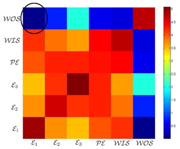
Visualization of the mutual information matrix generated by computing conditional mutual information between feature pairs. The encircled cell corresponds to the feature pair with the least conditional mutual information.
The input to the inference engine is the superpixelized version of each feature map. For every superpixel the engine outputs a probability estimate that the superpixel belongs to a tumor region. These inference probabilities are calculated using (7). In Fig. 5 we show a comparison between single channel and multichannel MRF segmentation. The multichannel MRF is based on the feature pair: (ℰ1,
). For single channel MRF we tested each of the individual features (ℰ1, ℰ2, ℰ3,
ℰ,
,
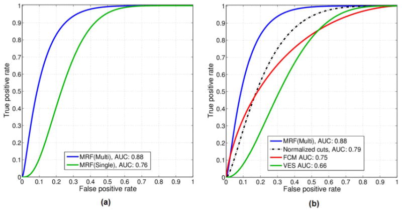
), and show the ROC for ℰ1 that gives the highest AUC. The inference probabilities are computed in a leave-one-out fashion i.e., the node potentials used in (7) are based on all images but the test image. The manual segmentation provided by the radiologist was used as ground-truth to assess the pixelwise agreement for ROC analysis. The ROC scores were derived from the inference probabilities. The multichannel MRF based method gives an AUC of 0.97 outperforming the best single channel MRF that gives an AUC of 0.89.
Fig. 5.

ROC comparison for breast tumor segmentation between multichannel and single channel MRF. The multichannel MRF using the feature pair (ℰ1,
) gives an AUC of 0.97 under the ROC curve as compared to 0.89 for single channel MRF based on the best individual feature (ℰ1).
We compare our method against the following segmentation algorithms.
C. Normalized Cuts
The normalized cuts algorithm [8] is a spectral graph theoretic method that is widely used for diverse segmentation applications [11]–[14]. It is an unsupervised segmentation technique that maximizes both the dissimilarity between different groups and the similarity within groups of pixels. The normalized cuts algorithm [8] models an image as a graph G = (V, E) and then aims to find a partition of the graph to minimize the cut cost normalized by the cost of the total edge connections to all the nodes in the graph
| (17) |
where cut(A, B) is the sum of edge costs that are being cut by the partition i.e., cut(A, B) = Σu∈A,v∈B w(u, v), and assoc(A, V) = Σu∈A,t∈V w(u, t) is the sum of costs for edge connections from nodes in A to all nodes in the graph. Minimizing normalized cut exactly is NP-complete but [8] proposed an approximate method that is able to solve the problem as a generalized eigenvalue system (see [8] for details). Usually the resultant eigenvectors are thresholded to obtain partitions of the image. However, in order to generate ROC curves we used the eigenvectors as the scores. We used the publicly available implementation of normalized cuts in our experiments [39]. We ran the normalized cuts algorithm using each of the six features and report the best performance in Fig. 6 that gives an AUC of 0.92 by using ℰ1 as an input.
Fig. 6.

ROC comparison for breast tumor segmentation. The multichannel MRF based segmentation method gives an AUC of 0.97 under the ROC curve as compared to 0.92, 0.88, and 0.60 for normalized cuts [8], FCM [15], [16] and FCM-VES [17], respectively.
D. Fuzzy C Means
Fuzzy C means (FCM) is a popular method for segmenting breast lesions from DCE-MRI images e.g., [15], [16]. FCM is an unsupervised learning technique [40] that aims to find a fuzzy partitioning of data points into clusters. If uki represents the extent of membership of the ith data point to the kth class, the FCM problem is to find all uki such that the following within group weighted squared Euclidean distance is minimized:
| (18) |
where b is a weighting exponent on each fuzzy membership, and μk is the weighted mean for kth class given the membership probabilities uki. To ensure that uki represent probabilities the above optimization is subject to the following constraints:
| (19) |
For our experiments we used Matlab's3 standard implementation of the FCM algorithm with b = 2. As input to the FCM algorithm we tested all the individual features and pairs of features, and FCM performed the best when ℰ1 and
were concatenated together to represent every pixel by a 2 × 1 feature vector. Connected component analysis was done on the FCM output and the largest component was selected as the segmented lesion [16]. The FCM probabilities were used as scores for generating the ROC curve which gave an AUC of 0.88 (Fig. 6).
E. FCM on Enhancement Variance
In [17], the authors first compute pixelwise variance of relative enhancement of breast MRI images. They then run FCM on the pixelwise variance. This method gives an AUC of 0.60 as shown in Fig. 6.
F. Performance Comparison
Fig. 6 presents the comparison of all the above approaches against our method. Our segmentation algorithm yields an AUC of 0.97 under the ROC curve for breast tumor segmentation compared to 0.92, 0.89, 0.88, and 0.60 for the normalized cuts algorithm, single channel MRF, FCM, and FCM on enhancement variance respectively. In Fig. 7, we show representative segmentation results of our algorithm (row 7), FCM [15] (row 3), FCM-VES [17], (row 4), normlaized cuts algorithm (row 5), and the best single channel MRF (row 6).
Fig. 7.
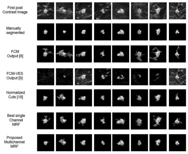
Qualitative comparison of segmentation results as overlayed on the first postcontrast image. Results of multichannel MRF approach (Row 7) are qualitatively more similar to the radiologist's provided ground truth (Row 2) as compared to traditional approaches (Row 3, 4), the normalized cuts algorithm (Row 5), and the best single channel MRF (Row 6).
V. Classification Experiments
In this section we investigate if better quality segmentation leads to better feature extraction and tumor characterization. In the specific application presented here we explore the role of segmentation in improved prediction of breast cancer prognosis as assessed by a validated gene expression assay (Oncotype DX). Although the outcome of the Oncotype assay is a continuous score, it has been shown that the benefit of a chemotherapy regimen starts becoming significant only in patients with an Oncotype score greater than 30, which is the high recurrence risk category [37]. As such, from a clinical perspective, the decision of low versus high recurrence risk is very important to choose women who are expected to benefit the most from adjuvant chemotherapy [41], [42]. Recent data indicate that in addition to distinguishing between benign and malignant findings, breast MRI kinetic tumor features and contrast enhancement patterns, are also significantly associated with histopathological findings that are indicative of subsequent prognosis and probability of relapse [43], [44]. To explore the effect of better segmentation we focus on the task of binary prediction of Oncotype scores as high or low, where we consider patients with scores greater than 30 in the high risk category.
A. Features for Classification
Here, we propose to investigate a rich set of kinetic statistics derived from DCE MRI images for the task of detecting patients with high recurrence risk. We extract the kinetic statistics in a two phase process: In the first phase the time to peak (TTP) for every pixel within the segmented tumor is computed. In the second phase we cluster the pixels based on their TTP values. In the dataset under consideration there are three post-contrast time points. TTP thus can have three discrete values and the clustering step results in three groups of pixels. It has been suggested that the heterogeneities in the contrast agent uptake can be used for tumor characterization [20], [45]. One way to interpret the kinetic heterogeneity is to divide the pixels into clusters of homogeneity. Therefore the idea behind clustering the pixels according to their TTP values is to group the pixels that show similar contrast uptake behavior such that statistics within these clusters of kinetic homogeneity could be explored. This step partitions the pixels into as many sets as the number of postcontrast time points, i.e., set i consists of pixels that achieve their peak enhancement at the ith postcontrast time point. Fig. 8 illustrates these partitions for an example case. In the second step, pixel-wise maps of the following features were computed: peak enhancement (PE), wash-in-slope (WIS), wash-out-slope (WOS), (Fig. 2). Based on these pixel groupings we compute partition-wise kinetic statistics as follows: Let ℳ be the pixel partitioning such that ℳk represents the membership mapping of pixel to its respective set. Given ℳ one can derive the following set-wise statistics.
Fig. 8.

Illustration of kinetic partitioning based on the TTP pixel-wise values. (a) Segmented lesion. (b) Set 1 pixels (yellow). (c) Set 2 pixels (blue). (d) Set three pixels (green). Set i consists of pixels that have their peak enhancement at the ith postcontrast time point.
-
Posterior probability of observing set i given the partition
(20) where δ(ℳk = i) is an indicator function that equals 1 when ℳk = i, and zero otherwise. N is the total number of pixels. These N pixels may come from an arbitrarily shaped segmentation mask specifying the lesion.
-
Mean value of feature map j for Set i
(21) where fj(k) is the value of the jth feature map for kth pixel, and the feature map can be either PE, WIS, or WOS.
- Variance of feature map j for Set i
(22)
Based on the above definitions, m pixel partitions and n feature maps would result into a total of m(2n + 1) features. For this dataset we had three postcontrast time points and based on the TTP values the pixels were partitioned into three sets (m = 3). Within these partitions we computed statistics for three feature maps (n = 3) i.e.,
ℰ,
, and
. This resulted in m(2n + 1) = 21 kinetic statistic features.
B. Single Feature Classifiers
To assess the classification performance of individual features we learned single feature classifiers to distinguish between the categories of low and high recurrence risk. For each feature we learned a leave-one-out binary decision stump classifier [46] using the individual feature values as scores for generating ROCs to evaluate the univariate performance of each feature. Table I shows the AUCs for the ROCs corresponding to each feature classifier. When features extracted from the output of the multichannel MRF algorithm were used for classification, 15 of the 21 features give AUCs greater or equal to 0.74 with an average AUC of 0.76. In Table I we also present comparison with single feature classification performance when features were extracted from the outputs of other segmentation techniques. For all the features, AUCs using the multichannel MRF based segmentation are higher than that for other approaches.
Table I.
Comparison of Single Feature Classification Performance in Terms of Area Under the ROC Curve When Outputs of Various Segmentation Strategies Were Fed Into the Feature Extraction Stage. In Column 1 Feature Names Follow the Notation of (20)–(22). E.g., μ(1, PE) Represents the Mean Feature Map Value of Peak-Enhancement for Set 1 Pixels. Columns 3–6 Show the Respective AUCs. In Each Column the Best Two Values Are Shown in Bold
| Feature | Multichannel MRF | Single Channel MRF | Normalized Cuts | FCM | FCM-VES |
|---|---|---|---|---|---|
(
 et = 1∣ℳ) et = 1∣ℳ) |
0.76 | 0.67 | 0.70 | 0.68 | 0.60 |
|
(
et = 2∣ℳ) |
0.76 | 0.68 | 0.69 | 0.66 | 0.64 |
|
(
et = 3∣ℳ) |
0.68 | 0.53 | 0.57 | 0.56 | 0.51 |
|
μ(1,
ℰ) |
0.77 | 0.69 | 0.71 | 0.65 | 0.57 |
|
μ(2,
ℰ) |
0.74 | 0.60 | 0.67 | 0.59 | 0.63 |
|
μ(3,
ℰ) |
0.58 | 0.52 | 0.51 | 0.57 | 0.54 |
|
σ2(1,
ℰ) |
0.75 | 0.67 | 0.69 | 0.67 | 0.55 |
|
σ2(2,
ℰ) |
0.62 | 0.58 | 0.56 | 0.53 | 0.51 |
|
σ2(3,
ℰ) |
0.59 | 0.52 | 0.51 | 0.57 | 0.55 |
|
μ(1,
) |
0.82 | 0.71 | 0.73 | 0.69 | 0.54 |
|
μ(2,
) |
0.78 | 0.70 | 0.72 | 0.70 | 0.60 |
|
μ(3,
) |
0.54 | 0.51 | 0.53 | 0.51 | 0.52 |
|
σ2 (1,
) |
0.74 | 0.64 | 0.68 | 0.65 | 0.54 |
|
σ2(2,
) |
0.75 | 0.69 | 0.70 | 0.67 | 0.59 |
|
σ2(3,
) |
0.64 | 0.52 | 0.62 | 0.56 | 0.60 |
|
μ(1,
) |
0.81 | 0.68 | 0.74 | 0.68 | 0.65 |
|
μ(2,
) |
0.76 | 0.64 | 0.67 | 0.66 | 0.54 |
|
μ(3,
) |
0.74 | 0.69 | 0.70 | 0.67 | 0.60 |
|
σ2(1,
) |
0.75 | 0.70 | 0.71 | 0.63 | 0.57 |
|
σ2(2,
) |
0.74 | 0.66 | 0.69 | 0.66 | 0.52 |
|
σ2(3,
) |
0.79 | 0.69 | 0.72 | 0.64 | 0.65 |
C. Multi-Feature Classifier
Using the features described in Section V-A we followed a leave-one-out sequential forward feature selection scheme. For each leave-one-out loop the feature selection was done as follows: Starting with a single feature, we sequentially added features, learned a linear support vector machine (SVM) on the training set corresponding to the current cross-validation fold, and kept adding the features till the incremental classification improvement dropped below a threshold (10−4) as compared to the previous feature set. This SVM classifier was tested on the left out example and the process was repeated for all cross-validation folds. Table II shows the frequency of selection for each of the features across all leave-one-out loops.
TABLE II.
Selection Frequencies of the Kinetic Statistic Features Over All the Classification Leave-One-Out Loops. For Every Leave-One-Out Loop a Sequential Forward Feature Selection Scheme Was Followed. In Column 1 Feature Names Follow the Notation of (20)(22). E.g., μ(1, PE) Represents the Mean Feature Map Value of Peak-Enhancement for Set 1 Pixels. Column 2 Shows the Selection Frequency of Each Feature Over All Cross Validation Folds
| Feature | Selection | Frequency |
|---|---|---|
|
(
et = 1∣ℳ) |
60/60 | (100.00%) |
|
(
et = 2∣ℳ) |
60/60 | (100.00%) |
|
(
et = 3∣ℳ) |
52/60 | (86.67%) |
|
μ(1,
ℰ) |
60/60 | (100.00%) |
|
μ(2,
ℰ) |
57/60 | (95.00%) |
|
μ(3,
ℰ) |
43/60 | (71.67%) |
|
σ2(1,
ℰ) |
54/60 | (90.00%) |
|
σ2(2,
ℰ) |
47/60 | (78.33%) |
|
σ2(3,
ℰ) |
42/60 | (70.00%) |
|
μ(1,
) |
58/60 | (96.67%) |
|
μ(2,
) |
60/60 | (100.00%) |
|
μ(3,
) |
39/60 | (65.00%) |
|
σ2(1,
) |
56/60 | (93.33%) |
|
σ2(2,
) |
60/60 | (100.00%) |
|
σ2(3,
) |
46/60 | (76.67%) |
|
μ(1,
) |
60/60 | (100.00%) |
|
μ(2,
) |
60/60 | (100.00%) |
|
μ(3,
) |
52/60 | (86.67%) |
|
σ2(1,
) |
60/60 | (100.00%) |
|
σ2(2,
) |
55/60 | (91.67%) |
|
σ2(3,
) |
53/60 | (88.33%) |
The ROC for the multi-feature classifiers when the output of different segmentation strategies were fed into the classification stage is shown in Fig. 9. The multi-feature classifier was able to distinguish between low and high recurrence risk patients with an AUC = 0.88 under the ROC curve when the proposed multichannel MRF segmentation strategy was employed, which was higher than that for other segmentation algorithms [Fig. 9(a) and (b)] which give lower AUCs of 0.79, 0.76, 0,75, 0.66 for normalized cuts, single channel MRF, FCM, and FCM-VES, respectively.
Fig. 9.
ROC Curves for the multi-feature SVM for classifying high versus low breast cancer recurrence risk. We get the highest AUC when the output of multichannel MRF segmentation method is fed to the feature extraction stage.
VI. Discussion
In Section IV-B, we derive features for our multichannel MRF that allow us to invoke conditional independence conditions by computing pairwise conditional mutual information between all possible pairs of features (ℰ1, ℰ2, ℰ3,
ℰ,
,
). Although data-driven, the selection of the first postcontrast enhancement (ℰ1) and wash-out slope (
) features as different observation channels of the multichannel MRF deserves attention. These two features capture different contrast agent uptake properties, each depending on different directions of vascular permeability e.g., ℰ1 represents the initial uptake of the contrast agent while
captures the drop in the uptake after the peak enhancement. As such they are less correlated with one another. The rest of the kinetic features are essentially derived from one another and are not expected to contain much uncorrelated information as is evident from the mutual information matrix of Fig. 4. As mentioned in (13) the conditional mutual information is conditioned on X i.e., the class of the node as to whether it belongs to tumor or background tissue. As such the selection of ℰ1 and
as good features for segmentation is also noteworthy as they capture properties of the contrast uptake in postcontrast MR images, which are shown to be different for background and tumor tissues [26], [15]. Although we use cross validation for generalization, and ℰ1,
do seem to represent good features for segmentation, their applicability for other cancer types requires more extensive validation.
In this study, we have investigated pairs of features for the multichannel MRF model. In principle, the multichannel MRF framework is applicable to any number of channels as long as the features satisfy conditional independence criterion. For the feature set currently in question (ℰ1, ℰ2, ℰ3,
ℰ,
,
), since only one pair satisfied the empirical test of conditional independence, adding more features from the same feature set would have essentially included features which already had significant mutual information with the selected pair (ℰ1,
). In the future, however, if more elaborate feature sets are explored, the possibility of experimenting with more channels remains open. We should also note that in Fig. 4, the diagonal of the mutual information matrix varies for different features, unlike what one would expect for a correlation matrix, where all diagonal values are same and equal to unity. The reason for this is that the mutual information of a random variable with itself represents the entropy of the variable and hence would vary from variable to variable [30].
It is worth mentioning that the work presented in [47] comes closest in concept to ours in terms of using multiple features for MRF. However, they assume a priori independence between features, whereas in our current work we present a principled method to derive conditionally independent features to arrive at appropriate features for the multichannel MRF. Moreover, [47] solves the MRF using an expectation maximization scheme, whereas we present how inference methods like loopy BP could be extended to multichannel MRFs. As mentioned in Section II-A, the BP algorithm is equivalent to minimizing the free energy of the graphical model, thereby arriving at better approximation of the distribution that needs to be recovered.
We should note that while learning the node potentials for our multichannel MRF we are modeling the features as a mixture of Gaussian PDFs. The features in and of themselves may not necessarily be Gaussians. However, it has been shown that the Gaussian mixture models provide good practical approximations to non-Gaussian noise processes [48]. That said, approximating the features with other distributions is a potential direction for future research.
We have also explored the impact of improved segmentation on the characterization and classification of breast cancer tumors. Our multichannel MRF segmentation method gives a much lower pixelwise false positive rate for the same true positive rate as depicted in the ROC curves of Fig. 6. This perhaps explains the improvement in classifying the Oncotype recurrence risk categories when tumors segmented by our algorithm are used for feature extraction. From a clinical perspective, the minimally-invasive estimation of recurrence risk from DCE-MRI features is an important question as it could become a useful decision tool for routing candidate patients to appropriate treatment options [49]. Our results suggest that improved segmentation could play a significant role in assisting this clinical decision. Moreover, the DCE-MRI features are currently extracted from a representative 2-D slice of the primary lesion. Kinetic partitioning of the entire 3-D volume of the lesion could potentially lead to richer statistics that may further improve the prediction of breast cancer recurrence in future work. Also, our current work focuses on accurately segmenting the tumor given a coarsely defined rectangular ROI. Adapting the existing method for a fully automated tumor detection is a potential topic for future research.
VII. Concluding Remarks
In this paper, we have presented a methodological framework for a multichannel extension of MRFs for breast tumor segmentation from DCE-MRI images. Using conditional independence we have shown that loopy belief propagation can solve a multichannel MRF as a single channel MRF. We have presented a method to search for optimal MRF features that satisfy conditional independence conditions by employing pairwise conditional mutual information. Using this framework we incorporate a kinetic observation model derived from DCE breast MR images into the multichannel MRF and demonstrate superior segmentation results (AUC = 0.97). Our multichannel MRF outperforms single channel MRF (AUC: 0.89) employing the best individual feature from the same pool of features as used by the multichannel MRF. Our approach also performs significantly better as compared to the well known normalized cuts segmentation algorithm and commonly used previous methods for breast tumor segmentation (AUCs: 0.92, 0.88, 0.60). Moreover, we also demonstrate that our improved segmentation leads to better feature extraction and tumor characterization with an application on predicting breast cancer prognosis as determined by a validated tumor gene expression assay. Specifically, when tumors segmented by our algorithm were fed into an SVM classifier, it was able to distinguish between women with high and low breast cancer recurrence risk with an AUC of 0.88 under the ROC as compared to AUCs of 0.79, 0.76, 0.75, and 0.66 for othersegmentation methods. The decision of low versus high recurrence risk is very important from a clinical perspective as it could enable to select patients that are expected to benefit the most from adjuvant chemotherapy [50], [41], [42]. We believe that the proposed methodological framework could also be extended to other imaging modalities and organs as well.
Acknowledgments
This work was supported by the Institute of Translational Medicine and Therapeutics (ITMAT) Transdisciplinary Program in Translational Medicine and Therapeutics under Grant UL1RR024134 from the National Center for Research Resources. The content of this work is the sole responsibility of the authors and does not necessarily represent the official views of the National Center for Research Resources or the National Institute of Health.
Footnotes
Color versions of one or more of the figures in this paper are available online at http://ieeexplore.ieee.org.
Matlab version 7.13,R2011b
Contributor Information
Ahmed B. Ashraf, Email: ahmed.ashraf@uphs.upenn.edu, Computational Breast Imaging Group (CBIG), Department of Radiology, University of Pennsylvania, Philadelphia, PA 19104 USA.
Sara C. Gavenonis, Computational Breast Imaging Group (CBIG), Department of Radiology, University of Pennsylvania, Philadelphia, PA 19104 USA
Dania Daye, Computational Breast Imaging Group (CBIG), Department of Radiology, University of Pennsylvania, Philadelphia, PA 19104 USA.
Carolyn Mies, Department of Pathology and Laboratory Medicine, University of Pennsylvania, Philadelphia, PA 19104 USA.
Mark A. Rosen, Computational Breast Imaging Group (CBIG), Department of Radiology, University of Pennsylvania, Philadelphia, PA 19104 USA
Despina Kontos, Computational Breast Imaging Group (CBIG), Department of Radiology, University of Pennsylvania, Philadelphia, PA 19104 USA.
References
- 1.Kass M, Witkin A, Terzopoulos D. Snakes: Active contour models. Int J Comput Vis. 1988;1(4):321–331. [Google Scholar]
- 2.Cootes TF, Taylor CJ, Cooper DH, Graham J. Active shape models—Their training and application. Comput Vis Image Underst. 1995 Jan;61:38–59. Online. Available: http://dl.acm.org/citation.cfm?id=206543.206547. [Google Scholar]
- 3.Tauber C, Batatia H, Ayache A. Quasi-automatic initialization for parametric active contours. Pattern Recognit Lett. 2010;31(1):83–90. [Google Scholar]
- 4.Saha S, Bandyopadhyay S. MRI brain image segmentation by fuzzy symmetry based genetic clustering technique. IEEE Congr Evol Comput. 2007:4418–4424. [Google Scholar]
- 5.Yoon OK, Kwak DM, Kim KHPDW. MR brain image segmentation using fuzzy clustering. Fuzzy Syst Conf Proc. 1999;2:22–25. [Google Scholar]
- 6.Zhang DQ, Chen SC. A novel kernelized fuzzy c-means algorithm with application in medical image segmentation. Artif Intell Med. 2004;32:37–50. doi: 10.1016/j.artmed.2004.01.012. [DOI] [PubMed] [Google Scholar]
- 7.Zhang Y, Brady M, Smith S. Segmentation of brain MR images through a hidden Markov random field model and the expectationmaximization algorithm. IEEE Trans Med Imag. 2001 Jan;20(1):45–57. doi: 10.1109/42.906424. [DOI] [PubMed] [Google Scholar]
- 8.Shi J, Malik J. Normalized cuts and image segmentation. IEEE Trans Pattern Anal Mach Intell. 2000 Aug;22(8):888–905. [Google Scholar]
- 9.Weiss Y. Segmentation using eigenvectors: A unifying view. Proc Int Conf Comput Vis. 1999:975–982. [Google Scholar]
- 10.Ng AY, Jordan MI, Weiss Y. Advances in Neural Information Processing Systems. Cambridge MA: MIT Press; 2001. pp. 849–856. [Google Scholar]
- 11.Gamio JC, Belongie S, Majumdar S. Normalized cuts in 3d for spinal MRI segmentation. IEEE Trans Med Imag. 2004 Jan;23(1):36–44. doi: 10.1109/TMI.2003.819929. [DOI] [PubMed] [Google Scholar]
- 12.Fowlkes C, Belongie S, Chung F, Malik J. Spectral grouping using the Nyström method. IEEE Pattern Anal Mach Intell. 2004 Feb;26(2):214–225. doi: 10.1109/TPAMI.2004.1262185. [DOI] [PubMed] [Google Scholar]
- 13.Zhao J, Zhang L, Zheng W, Tian H, Hao DM, Wu SH, He J, Liu X, Krupinski E, Xu G, editors. Health Information Science. Vol. 7231. New York: Springer; 2012. Normalized cut segmentation of thyroid tumor image based on fractional derivatives; pp. 100–109. LNCS. [Google Scholar]
- 14.Felzenszwalb P, Huttenlocher D. Efficient graph-based image segmentation. Int J Comput Vis. 2004;59:167–181. [Google Scholar]
- 15.Bhooshan N, Giger ML, Jansen SA, Li H, Lan L, Newstead GM. Cancerous breast lesions on DCE MR images: Computerized characterization for image based prognostic markers. Radiology. 2010;254(3):680–690. doi: 10.1148/radiol.09090838. [DOI] [PMC free article] [PubMed] [Google Scholar]
- 16.Chen W, Giger ML, Bick U. A fuzzy c-means (FCM)-based approach for computerized segmentation of breast lesions in dynamic contrast-enhanced MR images. Acad Radiol. 2006 Jan;13(1):63–72. doi: 10.1016/j.acra.2005.08.035. [DOI] [PubMed] [Google Scholar]
- 17.Lee S, Kim JH, Cho N, Park JS, Yang Z, Jung YS, Moon WK. Multilevel analysis of spatiotemporal association features for differentiation of tumor enhancement patterns in breast DCE-MRI. Med Phys. 2010;37:3940. doi: 10.1118/1.3446799. [DOI] [PubMed] [Google Scholar]
- 18.Ashraf AB, Gavenonis S, Daye D, Mies C, Feldman MD, Rosen M, Kontos D. A multichannel markov random field approach for automated segmentation of breast cancer tumor in DCE-MRI data using kinetic observation model. In: Fichtinger G, Martel AL, Peters TM, editors. MICCAI (3) Vol. 6893. New York: Springer; 2011. pp. 546–553. LNCS. [DOI] [PubMed] [Google Scholar]
- 19.Meltzer T, Globerson A, Weiss Y. Convergent message passing algorithms—A unifying view. Proc 28th Conf Uncertainty Artif Intell (UAI) 2009 [Google Scholar]
- 20.Hylton N. Dynamic contrast-enhanced magnetic resonance imaging as an imaging biomarker. J Clin Oncol. 2006;24:3293–3298. doi: 10.1200/JCO.2006.06.8080. [DOI] [PubMed] [Google Scholar]
- 21.Bishop CM. Pattern Recognition and Machine Learning (Information Science and Statistics) New York: Springer-Verlag; 2006. [Google Scholar]
- 22.Ravikumar P. Approximate inference, structure learning and feature estimation in Markov random fields: Thesis abstract. SIGKDD Explor Newsl. 2008 Dec;10(2):32–33. [Google Scholar]
- 23.Greig DM, Porteous BT, Seheult AH. Exact maximum a posteriori estimation for binary images. J R Stat Soc Ser B (Methodological) 1989;51(2):271–279. [Google Scholar]
- 24.Yedidia JS, Freeman WT, Weiss Y. Constructing free energy approximations and generalized belief propagation algorithms. IEEE Trans Inf Theory. 2005 Jul;51(7):2282–2312. [Google Scholar]
- 25.Cover TM, Thomas JA. Elements of Information Theory. New York: Wiley; 1991. [Google Scholar]
- 26.Chen W, Giger ML, Lan L, Bick U. Computerized interpretation of breast MRI: Investigation of enhancement-variance dynamics. Med Phys. 2004 May;31(5):1076–1082. doi: 10.1118/1.1695652. [DOI] [PubMed] [Google Scholar]
- 27.Ren X, Malik J. ICCV'03: Proc 9th IEEE Int Conf Comput Vis. Washington DC: 2003. Learning a classification model for segmentation; pp. 10–17. [Google Scholar]
- 28.Mori G, Ren X, Efros AA, Malik J. Recovering human body configurations: Combining segmentation and recognition. IEEE Comput Soc Conf Comput Vis Pattern Recognit. 2004;2:326–333. [Google Scholar]
- 29.Mori G. Guiding model search using segmentation. IEEE Int Conf Comput Vis. 2005;2:1417–1423. [Google Scholar]
- 30.Cover TM, Thomas JA. Elements of Information Theory. New York: Wiley; 1991. [Google Scholar]
- 31.Rosenblatt M. Remarks on some nonparametric estimates of a density function. Ann Mathe Stat. 1956;27:832–837. [Google Scholar]
- 32.Parzen E. On estimation of a probability density function and mode. Ann Math Stat. 1962;33:1065–1076. [Google Scholar]
- 33.Epanechnikov VA. Non-parametric estimation of a multivariate probability density. Theory Probabil Appl. 1969;14:153–158. [Google Scholar]
- 34.Botev ZI, Grotowski JF, Kroese DP. Kernel density estimation via diffusion. Ann Stat. 2010;38(5):2916–2957. [Google Scholar]
- 35.McLachlan GJ, Basford KE. Mixture Models. New York: Marcel Dekker; 1988. [Google Scholar]
- 36.Dempster A, Laird N, Rubin D. Maximum likelihood from incomplete data via the EM algorithm. J R Stat Soc. 1977;39(1):1–38. [Google Scholar]
- 37.Paik S, Tang G, Shak S, Kim C, Baker J, Kim W, Cronin M, Baehner FL, Watson D, Bryant J, Constantino JP, Geyer CE, Wickerham DL, Wolmark N. Gene expression and benefit of chemotherapy in women with node-negative, estrogen receptor-positive breast cancer. J Clin Oncol. 2006;24(23):3726–3734. doi: 10.1200/JCO.2005.04.7985. [DOI] [PubMed] [Google Scholar]
- 38.Yushkevich PA, Piven J, Hazlett HC, Smith RG, Ho S, Gee JC, Gerig G. User-guided 3D active contour segmentation of anatomical structures: Significantly improved efficiency and reliability. Neuroimage. 2006 Jul;31(3):1116–1128. doi: 10.1016/j.neuroimage.2006.01.015. [DOI] [PubMed] [Google Scholar]
- 39.Cour T, Shi K. Normalized Cuts Matlab Code. Online. Available: http://www.cis.upenn.edu/∼jshi/software/
- 40.Bezdek JC, Pal SK. Fuzzy Models for Pattern Recognition. New York: IEEE Press; 1992. [Google Scholar]
- 41.Paik S. Development and clinical utility of a 21-gene recurrence score prognostic assay in patients with early breast cancer treated with tamoxifen. Oncologist. 2007;12:631–635. doi: 10.1634/theoncologist.12-6-631. [DOI] [PubMed] [Google Scholar]
- 42.Paik S, Shak S, Tang G, Kim C, Baker J, Cronin M, Baehner FL, Walker MG, Watson D, Park T, Hiller W, Fisher ER, Wickerham DL, Bryant J, Wolmark N. A multigene assay to predict recurrence of tamoxifen-treated, node-negative breast cancer. N Eng J Med. 2004;351:2817–2826. doi: 10.1056/NEJMoa041588. [DOI] [PubMed] [Google Scholar]
- 43.Szabó BK, Aspelin P, Wiberg MK, Tot T, Boné B. Invasive breast cancer: Correlation of dynamic MR features with prognostic factors. Eur Radiol. 2003;13:2425–2435. doi: 10.1007/s00330-003-2000-y. [DOI] [PubMed] [Google Scholar]
- 44.Matsubayashi R, Matsuo Y, Edakuni G, Satoh T, Tokunaga O, Kudo S. Breast masses with peripheral rim enhancement on dynamic contrast-enhanced MR images: Correlation of MR findings with histologic features and expression of growth factors. Radiology. 2000;217:841–848. doi: 10.1148/radiology.217.3.r00dc07841. [DOI] [PubMed] [Google Scholar]
- 45.Chen W, Giger ML, Bick U, Newstead GM. Automatic identification and classification of characteristic kinetic curves of breast lesions on DCE-MRI. Med Phys. 2006 Aug;33(8):2878, 87. doi: 10.1118/1.2210568. [DOI] [PubMed] [Google Scholar]
- 46.Ai WI, Langley P. Induction of one-level decision trees. Proc 9th Int Conf Mach Learn. 1992:233–240. [Google Scholar]
- 47.Deng H, Clausi D. Unsupervised image segmentation using a simple MRF model with a new implementation scheme. Proc 17th Int Conf Pattern Recognit. 2004 Aug;2:691–694. [Google Scholar]
- 48.Kozick R, Sadler B. Maximum-likelihood array processing in non-Gaussian noise with Gaussian mixtures. IEEE Trans Signal Process. 2000 Dec;48(12):3520–3535. [Google Scholar]
- 49.Mook S, Schmidt MK, Rutgers EJ, van de Velde AO, Visser O, Rutgers SM, Armstrong N, van'tVeer LJ, Ravdin PM. Calibration and discriminatory accuracy of prognosis calculation for breast cancer with the online adjuvant! program: A hospital-based retrospective cohort study. Lancet Oncol. 2009;10:1070–1076. doi: 10.1016/S1470-2045(09)70254-2. [DOI] [PubMed] [Google Scholar]
- 50.Ginsburg O, Ghadirian P, Lubinski J, Cybulski C, Lynch H, Neuhausen S, Kim-Sing C, Robson M, Domchek S, Isaacs C, Klijn J, Armel S, Foulkes WD, Tung N, Moller P, Sun P, Narod SA. Smoking and the risk of breast cancer in BRCA1 and BRCA2 carriers: An update. Breast Cancer Res Treat. 2009;114:127–135. doi: 10.1007/s10549-008-9977-5. [DOI] [PMC free article] [PubMed] [Google Scholar]